Application of Neural Networks in Character Recognition - CiteSeerX

International Journal of Computer Applications (0975 – 8887) Volume 52– No.12, August 2012

Application of Neural Networks in Character Recognition V. Kalaichelvi

Ahammed Shamir Ali

Assistant Professor Dept of Electronics & Instrumentation Engg BITS PILANI, DUBAI CAMPUS

Student BITS PILANI, DUBAI CAMPUS

ABSTRACT

2. ARTIFICIAL NEURAL NETWORKS

With the recent advances in the computing technology, many recognition tasks have become automated. Character Recognition maps a matrix of pixels into characters and words. Recently, artificial neural network theories have shown good capabilities in performing character recognition. In this paper, the application of neural networks in recognizing characters from a printed script is explored. Contrast to traditional methods of generalizing the character set, a highly specific character set is trained for each type. This can be termed as targeted character recognition.

Artificial Neural Networks (ANN) is a computational model that is based on how human brain interacts and learns new things. ANN consists of a number of simple units that work parallel through weighted connections. Learning algorithms adjust these weights as it processes information. Once fully trained, the weights act as a torch lighting the way as information passes till the output nodes.

Pattern Recognition, Character Recognition, Artificial Neural Networks.

The algorithm used in this paper is BPN (Back Propagation Network). The BP algorithm determines the weight for a multilayer ANN with feed-forward connections. During the learning phase, the computation is done by minimizing a mean square difference between the desired output and the actual output [5].

Keywords

2.1 Mathematical Model

General Terms

Neural Networks, Character Recognition, Back Propagation

1. INTRODUCTION Optical Character Recognition (OCR) refers to identifying printed characters as digitally recognizable form (such as ASCII) [1]. From preserving ancient manuscripts to helping blind people read (by using text-to-speech algorithms), the advantages are numerous. There are various ways to do this. Traditionally, this was possible only through complex algorithms that had very little tolerance to errors. These algorithms required more computational power and processing time. In spite of these drawbacks, it is extremely difficult to code. Traditional algorithms included sharp feature extraction and comparison to a stencil. This had many flaws and a little deviation from stencil had disastrous results. Another disadvantage is that the stencil has to be hard coded and addition of new characters would mean reprogramming the whole software. Handwritten character recognition has additional problems such as the variability in handwriting, similarity, and different styles. Omid Rashnodi et al have suggested box approach in Persian Handwritten digits Recognition [2]. With the advancements in Neural Networks, pattern recognition has had a huge leap. This reduces coding to minimal. There are many algorithms based on ANN to achieve OCR. This paper aims at improving the accuracy and efficiency of the existing Neural Network algorithms. Given the wide variety of applications, it is very important to develop a reliable and a flexible way to recognize characters. Sameeksha Barv has implemented OCR using neural networks. In that paper, each typed English letter is represented by binary numbers that are used as input to a simple feature extraction system whose output, in addition to the input, are fed to an ANN [3]. A comparison study of backpropagation neural network and leaning vector quantization is analyzed by Anuja P. Nagare [4]

v w 1

2

3

Output Layer y (θ)

Input Layer x (t)

Hidden Layer z (τ)

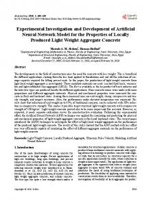
Fig 1: Architecture of ANN model Figure 1 shows the basic structure of an ANN model. For each training values, a series of steps are done. These steps can be broken down mainly into Forward Pass and Backward Pass. At the beginning of training, the weights are randomly initialized [6]. The nomenclatures used in the algorithm are given below:

xi

– Input value

vij

– Weight from input to hidden

1

International Journal of Computer Applications (0975 – 8887) Volume 52– No.12, August 2012

v0 j

– Weight of bias node from input to hidden

z _ inj – Weight from input to hidden node

z j – Weight output from hidden node w jk - Weight of bias node from hidden to output

w0 k - Weight of bias node from hidden to output y _ inj – input to hidden node

n

z j  f z _ in j 

 j   _ in j f z _ in j  ………………………. (6) vij   j xi

………………………. (7)

v0 j   j

The old weights are then added with the change to get the updated weights.

w0 k new  w0 k old   w0 k

During the forward pass, information from the input layer goes to output layer through hidden layer. Each input node in the input layer is loaded with the values that are given for training. And for each input pattern a desired output is also supplied. Each hidden unit sums up all incoming values and its bias and then is passed to an activation function f(x).

i 1

………………………. (5)

k 1

w jk new  w jk old   w jk

y j – Final output value

z _ in j  v 0 j   xi vij

m

 _ in j    k w jk

………………………. (1)

The output from the hidden node is passed to every output node. The output node sums up the value from each hidden node and then passes to activation function.

………………. (8)

3. METHODOLOGY The entire process can be broken down into Pre-processing, Feature Extraction, and then passing into ANN for training and simulation. These steps are visualized in fig 2. Segmentation Scaling Line Detection

Normalization Binarization Thinning

Pre Processing

Feature Extraction

Training Analysis Simulation

ANN Modeling

p

y _ ink  w0 k   z j w jk yk  f  y _ ink 

j 1

………………………. (2)

3.1 Pre-processing

This marks the end of Forward Pass. The backward pass begins with determining the error. The error is the difference between the desired and actual value

tk  yk . This error

has to be distributed backwards to each hidden node. In order to find that it is passed through the derivative of activation function.

 k  tk  yk  f  y _ ink  …………………… (3) Once

 k is

found, the change in weight can be easily

computed as:

w jk   k z j w0 k   k

Fig 2: Flowchart of Pattern Recognition system

…………………….. (4)

Learning rate determines how fast the model learns. A small value would result in a long training time where as a high value would make the model ineffective when there are variations in the input pattern.

Prior to ANN modeling, it is important that the images are in good quality. This enhances the image and decreases noise and distortion. This helps in achieving higher accurate results. It is essential in any OCR system that a preprocessing stage exists [7].

3.1.1 Normalization This helps to decrease the noise in the image by performing a local averaging operation on a 5 X 5 neighborhood. In order to achieve this, a median or mean filter can be used. To achieve minimal blurring, median filter is used.

3.1.2 Binarization Local binarization is then carried out in the resulting image. Since the color information is irrelevant, this gives us uniformity between the samples. This also reduces computational power as it has to deal with only 2 colors.

3.1.3 Thinning Thinning reduces the width of similar pixels to 1 pixel. Thinning is done with the help of edge detection by sobel’s method. Thinning reduces redundancy and makes the characters uniform. Other pre-processing techniques such as Skew detection/correction, histogram matching, etc. could also be done.

Updating the weights between the input and hidden layers require more calculations.

2

International Journal of Computer Applications (0975 – 8887) Volume 52– No.12, August 2012

3.2 Feature Extraction Feature extraction in OCR using Neural Networks primarily refers to the extraction of each character from the image.

3.2.1 Segmentation Segmentation refers to isolation of each character from others. It is done by drawing the smallest rectangle drawn around the characters. This is done using the regionprops function in Matlab. The BoundingBox property of regionprops contains the coordinates of the rectangle. This can be reshaped to fit the type of dataset using reshape function. Prior to using regionprops, it is essential that any spaces are removed or any discontinuity within each character or else it would be treated as separate ones. This can be achieved by dilation and filling up the holes. This is achieved by imfill and imfill function. Dilation fills up the small gaps in boundaries and imfill fills up the boundaries. Now it is possible to easily generate draw boxes around the blocks, the coordinates of this can be used to extract the character.

3.2.2 Scaling The image thus extracted is scaled into a 7 X 5 matrix irrespective of the size. The image is scaled up/down to attain uniformity. Scaling has to be done carefully preserving the important features. This is done using a separate user defined function.

3.2.3 Detection of Line If the image contains multiple lines with no proper justification (e.g. handwritten text), then there is a good chance that Ilabel function would pick up the characters in the wrong order. In order to tackle this, the y coordinates are compared and sorted in a special way. A local threshold is calculated to determine the average difference between two adjacent lines. This threshold then determines the sorting criteria.

from the data itself, i.e., the training set consists of all the individual letters that make up the document. Each font/ handwriting has its uniqueness. And this unique features associated with a character remains the same throughout the scripture. The training set can be further optimized by excluding any character that the author never uses. This reduces redundancy. Analysis of a standard 26 letters is done and documented. This can be used as starting point to reduce time. Some standard models can be trained for quick tasks. During training the models are trained with a custom training set. A custom training set is a tailored set of all characters that makes up the full document. A common training set is possible if the constituents are known beforehand. For example, English alphabets. A custom training set can increase accuracy to a wide extent. For example, if the document does not contain any punctuation mark other than period and comma, then all the other punctuation marks become redundant. A custom training set reduces this and includes only which are found in the document. This means the model would not have to confuse between unused symbols.

4. SIMULATION STUDIES 4.1 Case study 1 An image containing the text “THE QUICK BROWN FOX JUMPS OVER THE LAZY DOG.” is selected. The font used was Calibri, text size of 20 and spacing of 2.2. For simplicity, all letters were capitalized. The training set consisted of the same font and size from A to Z with full stop. As discussed earlier, the custom training set is what makes this more accurate. Figure 3 explains how all the alphabets are included in it. The word “DOG” has been purposely moved to the next line so as to check the line detection in the program. Simulation studies are carried out using MATLAB software [8-11]

3.2.4 Detection of Space Since each character is segmented by finding the space between them it is not possible to find the actual space between words. In order to detect space, before passing each character to the ANN, the difference between the xcoordinates of adjacent characters are compared with a threshold value to see if it’s an actual space. Threshold value is calculated locally. The spaces between each character is calculated and sorted in descending order. The difference between these sorted values determines which one is an actual space (space between words) and which one is not. The lowest value acts as threshold.

Fig 3: Printed Characters for Case Study 1

4.2 Analysis of Simulation Results 4.2.1 Training Set The idea behind targeted OCR is getting a tailored training set. Training set contains all 26 alphabets and the end punctuation. Since only capital letters are used, the training set need not contain any small letters as shown in Figure 4.

3.3 ANN Model The ANN model selected is a Feed Forward Back Propagation Network. The information is passed in Forward direction and Error is propagated backwards. The optimal number of hidden layers and nodes has to be selected based on simulation and training results. Typically the model contains 1 Input layer, 1 hidden layer and 1 Output layer. Input layer consist of 35 nodes (7 X 5). No. of Output and Hidden nodes vary according to the situation. Output nodes depend on the separate characters that make up the document. A dynamic model is better suited for a targeted OCR than a generalized one. In this way better accuracy can be attained as the model is trained particularly for the dataset. Training set is

Fig 4: Training set for Character Recognition

4.2.2 Training Number of nodes can now be fixed as the training set is ready. There are 35 input nodes, representing each pixel of the 7 X 5 character. There are 27 output nodes meaning hidden nodes can be around half of 27. Hidden nodes were fixed at 11. The activation function used was Logsig. Any of these parameters can be changed to suit a particular case. In order to train the NN model, certain parameters have to be fixed. The optimal values are found out by simulation analysis. Important

3

International Journal of Computer Applications (0975 – 8887) Volume 52– No.12, August 2012 parameters are Learning Rate (LR), Epochs, and Momentum Constant (MC). Performance goal was set at 1e-09. Once trained, the model can be used to recognize any number of images with the same building blocks (characters) [12-13].

4.2.3 Optimum Value The parameters of the model ultimately decide how accurate and fast the result will be. It is essential to do some analysis before fixing the values. The optimum value can be found by looking at the Performance attained and time taken. Initial value for the model has been set as LR = 0.01, MC = 0.95, Maximum Epochs = 6000.

4.2.3.1 Analysis of Learning Rate In order to analyze learning rate, the momentum constant and maximum epochs had been kept constant. Typical values of LR range from 0 to 1 and hence 6 values (0.01, 0.1, 0.25, 0.5, 0.75, and 1) were taken into account. The observations are recorded below. Table 1: Analysis of Learning Rate Analysis Of Learning Rate (Keeping MC at 0.95) LR Epoch Goal Met Time (s)

0.01 6000 No 29

0.1 3681 Yes 26

0.25 4137 Yes 23

0.5 5264 Yes 27

0.75 2846 Yes 16

1 3740 Yes 21

From Table 1, it is clear that LR at 0.75 produced the best result in terms of both time and performance. The performance curve (Figure 5) also suggests that this has a faster convergence rate in comparison with other LR values. The average time taken to complete is very low compared to rest. The error was found to be 9.92e-10 and was even lower than the goal. The average performance point was 0.444 and was clearly the most suitable choice. A further increase in learning rate also means that the NN model would treat even minor changes as different input.

4.2.3.2 Analysis of Maximum Epochs Maximum number of epochs is an important factor in determining the average training time. If the performance goal cannot be met, then the termination is triggered by either minimum gradient or by the number of epochs. Minimum gradient is fixed and hence the average time is entirely dependent on the maximum number of epochs. A very low epoch would result in an unfinished performance and a very high number would result in wastage of time if the performance is not met. Unlike the other parameters, this is judged by counting the no. of trials to success. It can also be calculated on the number of successful attempts for each epoch. The training is regarded as failure when the performance goal is not met.

Table 2: Analysis of Max. Epochs Analysis Of Maximum Epochs (MC = 0.95, LR=0.75) 8000

7000

6000

5000

4000

1

1

2

3

4

Epoch

3417

2495

4486

3386

2821

Time

18

14

23

27

16

Max Epoch Failures

From Table 2, it is clear that that the no. of failures is constant when maximum epoch is above 7000 and hence keeping a higher value does not make any sense. Therefore, max epoch of 7000 has been selected as the optimal combination. Out of 10 trials, there was only 1 failure when the maximum epoch was set at 7000. The analysis was done keeping LR and MC constant. LR value is update from the previous analysis and is set at 0.75 whereas MC is set at 0.95 which was the initial value.

4.2.3.3 Analysis of Momentum Constant Since the LR and Maximum Epoch are optimized, the training time now solely depends upon the momentum constant. Like learning rate, it determines how fast it converges. MC reduces the chance of giving wrong inputs (while learning) when unusual inputs are processed. In a way MC eases the function of Learning Rate. Since LR is kept at 0.75, it is essential to choose a value greater than 0.5 so that in effect the LR is reduced to half. If MC=0, there is no effect of MC and if MC=1, there is no effect of LR. Both these conditions are not desirable and hence the values of MC range from 0.5 to 0.95. Table 3: Analysis of Momentum Constant Analysis Of Momentum Constant (Keeping LR at 0.75) MC Epoch Goal Met Time (s)

0.5 3643 Yes 21

0.65 7000 No 34

0.8 2347 Yes 15

0.95 4357 Yes 22

From Table 3 it is very clear that the optimum value is 0.8, as the average training time is just 15s (the lowest time with any other combination). The performance is 0.454 and suggests improvement from the original case when LR was kept at 0.75. The performance curves (Fig 5) converge much quickly and show steepness at regular interval. The mean squared error is dropped to a staggering 10-2 at just about 40 epochs, which means even if the goal is met, this would give the best results

4

International Journal of Computer Applications (0975 – 8887) Volume 52– No.12, August 2012 Following the exact steps a 90% accuracy was obtained. After tweaking the space and line detection and with low learning rate, 100% accuracy was obtained. This means a low value of LR favors handwritten characters. Figure 9 shows the simulation results of handwritten character using Matlab software. The training time took only 11 seconds to complete with an LR of 0.5.

Fig 5: Performance Curve for the best training

5. RESULT The training was carried out and was highly successful. In addition to meeting the performance goal, it only took 21 seconds to finish the training. The result is shown below. The problem was then presented to the trained model to recognize the characters. It came out with 100% accuracy. The simulation results using Matlab software is shown in Figure 6.

Fig 9: Simulation Result of Handwritten Character

6. CONCLUSION OCR has a wide variety of applications and there exists various ways to achieve it. In the present work, an attempt has been made to implement neural network technique for character recognition. Neural Network is a very effective method to decipher any character of any language given the right set of training. In cases such as preserving old manuscripts where accuracy is more important, then this method can be employed. Also it is possible to improve the accuracy by adding probability to each character. For example a capital Q is very less likely to be found. Q is often mistaken with O in most of the OCR software. The results then can be forwarded for human review as nothing is full proof.

Fig 6: Simulation Result of Problem 1 All the characters were correctly decoded. The spacing detection and new line detection was accurate. To test the accuracy with handwritten characters, the following problem (Figure 7) was taken as the sample.

Fig 7: Handwritten Character In order to recognize the characters, the training set was created from the same handwriting. In order to test the effectiveness of the present approach, full alphabets were trained though adhering to the principle would require only 8 characters. The training set is shown in Figure 8.

Custom training set is more effective than a Universal trained set. For better results, different parameters should be adjusted for printed character recognition and handwritten characters. This also means addition of new characters for recognition is easy. Certain improvements such as a GUI based interface that can make training set by choosing the individual character would automate the process and save large amount of time. Many custom training set can be tweaked and saved for specific purposes. These can be used on less important documents and get accurate results.

7. REFERENCES [1] AJ Palkovic. “Improving Optical Character Recognition.” Proceedings of the 2nd Villanova University Undergraduate Computer Science Research Symposium (CSRS 2008). December 5, 8 & 10, 2008, [Online], USA. [2] Omid Rashnodi, Hedieh Sajedi and Mohammad Sanjee Abadesh. “Article using Box approach in Persian Handwritten Digits Recognition.” International Journal of Computer Applications, vol.32, no.3, pp 1-8.

Fig 8: Training set for Handwritten Character

[3] Sameeksha Barve. “Optical Character Recognition Using Artificial Neural Network.” International Journal of

5

International Journal of Computer Applications (0975 – 8887) Volume 52– No.12, August 2012 Advanced Research in Computer Engineering & Technology”, Vol.1, No.4, 2012. [4] Anuja P. Nagare. “License Plate Character Recognition System using Neural Network.” International Journal of Computer Applications, Volume 25, No.10, July 2011, pp. 36-39. [5] V.Kalaichelvi, D.Sivakumar and R.Karthikeyan. “Prediction of flow stress of 6061 Al-15% SiC MMC composites using adaptive network based fuzzy inference system.” International Journal of Materials and Design, volume 30, issue 4, April 2009, pp 1362-1370. [6] Laurene Fausett. “Fundamentals of Neural Networks: Architecture, Algorithms and Applications.” Prentice Hall, 1994. [7] S.N.Sivanandam, S.Sumathi and S.N.Deepa. “Introduction to Neural Networks using MATLAB.” Tata McGraw Hill, 2006. [8] Neural Network toolbox user’s guide, The Math works Inc.; 1998, Version 4.0.

[9] Danilo Octavio [Online]. Available: http://wwweurope.mathworks.com/matlabcentral/fileexc hange/18169-optical-character-recognition-ocr. 2009. [10] Li, Fuliang and Gao, Shuangxi. “Character Recognition System Based on Back-propagation Neural Network”, International Conference on Machine Vision and Human-machine Interface. 2010. [11] Hussain, B and Kabuka, M. R., “A novel feature recognition neural network and its application to character recognition”, IEEE Transactions of Pattem Recognition and Machine Intelligence, Vol. 16, No.1, 1994. [12] Yingqiao Shi, Wenbing Fan, Guodong Shi. “The Research of Printed Character Recognition based on Neural Network”, Fourth International Symposium on Parallel Architectures, Algorithms and Programming. 2011. [13] Srinivasan, B and Mani, N. “Application of artificial neural network model for optical character recognition”, Systems, Man, and Cybernetics, 1997.

..

6