Jun 21, 1993 - niques can be considered to build nonlinear controllers with improved performances. In this paper, we first consider a single, isolated, gen-.
Neural Networks, ¥ol 7, No 1, pp 183-194, 1994 Copyright © 1994 Elsevier Science Ltd Printed in the USA. All rights reserved 0893-6080/94 $6 00 + 00
Pergamon
CONTRIBUTED ARTICLE
Application of Neural Networks to Load-Frequency Control in Power Systems FRAN(~OISE BEAUFAYS, 1 YOUSSEF A B D E L - M A G I D , 2 AND BERNARD WIDROW 1 ~StanfordUniversityand 2KingFahad Universityof Petroleum and Minerals (Received 8 June 1992; revtsed and accepted 21 June 1993)
Abstract--This paper describes an apphcatton o f layered neural networks to nonhnear power systems control. A single generator unit feeds a power hne to various users whose power demand can vary over trine. As a consequence o f load variatwns, the frequency o f the generator changes over ttme A feedforward neural network is trained to control the steam admtsston valve o f the turbme that drtves the generator, thereby restoring the frequency to its nominal value. Frequency transients are minimized and zero steady-state error is obtained The same techmque is then applied to control a system composed o f two single umts tted together through a power hne Electrw load variations can happen independently m both units. Both neural controllers are trained wtth the back propagatwnthrough-time algorithm Use of a neural network to model the dynamtc system ts avoided by introducing the Jacoblan matrices o f the system in the back propagation chain used in controller training
Keywords--Power system, Load-frequency control, Feedforward neural network, Back propagation-through-time. shoot in the dynamic response of the overall system (Elgerd, 1982). This type of controller is slow and does not allow the control designer to take into account possible nonlinearities in the generator unit. We propose in this paper a neural network loadfrequency controller. The neural network makes use of a piece of information that is not used in conventional controllers: an estimate of the electric load perturbation (i.e., an estimate of the change in electric load when such a change occurs on the bus). This load perturbation estimate could be obtained either by a linear estimator or by a nonlinear neural network estimator. In certain situations, it could also be measured directly from the bus. We will show by simulation that when a load estimate is available, the neural network can achieve extremely good dynamic response. The same neural network technique is then extended to control a two-area system (i.e., two generator units linked together by a tie-line) where electric load perturbations can happen independently in both areas. The two neural controllers are adapted using the back propagation-through-time algorithm (Nguyen & Widrow, 1989, 1990; Werbos, 1990). The system to be controlled, the d y n a m i c plant, is represented by its state space equations. An error signal is defined at the output of the dynamic plant as the difference between the state vector of the plant and a desired state vector. Back propagation of the error vector through the plant state space equations is effected by means of a multiplication
1. I N T R O D U C T I O N Control and stability enhancement of synchronous generators is of major importance in power systems. Different types of controllers based on classical linear control theory have been developed in the past (Elgerd, 1982; Anderson & Fouad, 1977, Debs, 1988; Wood & Wollenberg, 1984). Because of the inherent nonlinearity of synchronous machines, neural network techniques can be considered to build nonlinear controllers with improved performances. In this paper, we first consider a single, isolated, generator unit connected to a power line or electric bus that serves different users. Variations in the power demand of the users cause the electric load on the bus to change over time. As the load varies, the frequency of the generator unit varies. To bring the steady-state frequency back to its nominal value after a given load variation, a control system is designed that acts on the setting of the steam admission valve of the unit turbine. It is of great importance to eliminate frequency transients as rapidly as possible. Most load-frequency control systems are primarily composed of an integral controller. The integrator gain is set to a level that compromises between fast transient recovery and low over-
Requests for reprints should be sent to Bernard Widrow, Information Systems Laboratory, Department of Electrical Engineering, Stanford University, Stanford, CA 94305-4055.
183
184
F BeauJay~. Y Abdel-Magtd. and B Wtdrow ' I
. . . . . .
I
Integral Controller
Ch,.s~
~
F]OW(~"
~-I~ ~sh
S ~eed Regulator
close I Steam Adl~llon Valve open
/
C~era~or FrequenCy Fr~tu*acy Fluctuation Af
"l l
l~qucncy Set Point =60Hz
L~
F
~.~.
Hydrauhc
Turbine
ne
Generator
Amplifier
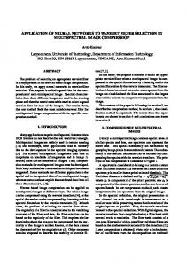
FIGURE 1. Conventional single-area system: simplified functional diagram.
of the error vector w]th the Jacobian matrix of the plant (a matrix containing the derivatives of the elements of the state transition matrix with respect to the state variables of the plant) (Piche & Widrow, 1991 ). The resulting signal is then back propagated through the neural network controller, and the adaptwe weights of the controller are adjusted according to the back propagation algorithm. Introducing Jacobmn matrices in the back propagation chain can be done whenever the state space equations of the plant are known a priori, and this avoids the introduction and training of a neural network plant model. The next section of this paper describes the systems under study and shows how conventional integral controllers are used to control such plants. Following sections describe the neural networks used to control the plants and present simulation results. Models, equations, and orders of magnitude of parameters are m accord with examples in the classic book by O. Elgerd, Electrtc Energy Systems Theory (Elgerd, 1982, chap. 9, sections 9.3 and 9.4). 2. P L A N T M O D E L S AND C O N T R O L BY CONVENTIONAL MEANS
2.1. Automatic Load-Frequency Control in Single-Area Systems In a single-area system, ~mechanical power is produced by a turbine and delivered to a synchronous generator serving different users. The frequency of the current and voltage waveforms at the output of the generator
For sake of clarity, we restrict the conceptof area to pertain to a system containing one single generatoralthough, m practice, the wordarea generallyrefersto a systemcontainingmany parallel-workmg generators( Elgerd, 1982)
is mainly determined by the turbine steam flow. It is also affected by changes in user power demands that appear, therefore, as electric perturbations. If, for example, the electric load on the bus suddenly increases, the generator shaft slows down, and the frequency of the generator decreases. The control system must immediately detect the load variation and command the steam admission valve to open more so that the turbine increases its mechanical power production, counteracts the load increase, and brings the shaft speed and hence the generator frequency back to its nominal value. A simplified functional diagram of a conventionally controlled power system is shown in Figure 1. A brief explanation of the diagram follows (a more detailed description can be found in Elgerd, 1982). Steam enters the turbine through a pipe that is partially obstructed by a steam admission valve. In steadystate, the opening of the valve is determined by the posiUon of a device called the speed changer (upper left corner in Figure 1). Its setting (points H or A in Figure 1 ) fixes the position of the steam valve through two rigid rods ABC and CDE. The reference value, or set-point, of the turbine power in steady-state is called the reference poner and is denoted by Pref. When the load on the bus suddenly changes, the shaft speed is modified, and a device called the speed regulator acts through the rigid rods to move the steam valve. Note that a similar effect could be producted by temporarily modifying the reference power (which justifies the name speed changer). In practice, both control schemes are used simultaneously. Amplifying stages (generally hydraulic) are introduced to magnify the outputs of the controllers and produce the forces necessary to actually move the steam valve. The speed regulator is a proportional controller of gain 1/R (that is, the deflection in B, AXB, is proportional to 1/R times the frequency fluctuation Af ) . In
Apphcatmn of N N to Power Systems Control
185
conventional systems, an integral controller of gain/£i sums the frequency fluctuations A f (point G ) and uses the result (point H) as a control signal to the speed changer to raise or lower the reference power. By combining these two control loops, we get a parallel PI (proportional-integral) controller capable of driving frequency fluctuations to zero whenever a step-load perturbation is applied to the system (Elgerd, 1982). Because most devices in power systems are extremely nonlinear, one usually likes to linearize the plant and to think of different variables in terms of their fluctuations about given operating points. Nonlinearities are then modeled by making the parameters of the linearized system functions of the operating point. The resuiting small signal models consist of linear operators having variable parameters whose values depend upon the state of the system. The last step in modeling consists of replacing all small signals by their Laplace transform and to represent the linearized devices by transfer functions. Before going any further, let us define the notation. A of some variable represents the difference between the variable and its nominal value. Lowercases are used for time signals, and uppercases for their Laplace transforms. For example, A f ( t ) represents the generator frequency relative to its nominal value, that is, A f ( t ) = f ( t ) - f n o m m a l = f ( t ) - 60 Hz, and AF(s) represents the Laplace transform of Af(t). A Laplace domain small signal model of the singlearea system is given in Figure 2. Points A, B, C, D, E, F and G of Figure 1 are also shown here to help relate the figures. Starting from point A in Figure 1, the fluctuation in reference power Ap~r (i.e., the output of the speed changer) is added to the output of the speed regulator (point B) to produce a global control signal (point C), which is instantaneously transmitted to the input of the hydrauhc amplifier (point D). For simplicity, the hydraulic amplifier is modeled by a firstorder transfer function whose output is the fluctuation in hydraulic amplifier power APtt(s). The turbine is also modeled by a first-order transfer function. Its input is the hydraulic amplifier output APn(s), its output is the turbine mechanical power APT(s). The change in variable load (lower right corner in Figure 1) is symbolized by an electric perturbation, APe(s), and can be modeled as an input perturbation to the generator ~
~
bTrequency
(Elgerd, 1982). The input to the generator model in Figure 2 is thus the sum of the turbine output power and the electric perturbation. The generator is modeled by a first-order transfer function. Its output, the frequency fluctuation AF(s) (point G), is used to drive the speed regulator and the integral controller. To simulate the dynamic plant in a C-programming environment, we derive its discrete-time state space equations. Referring to Figure 2 and expressing the outputs of the generator, turbine, and amplifier as functions of their inputs, inverting the Laplace transforms, and discretizing the time functions, we obtain the following discrete-time state space equations: L
Af(nTs + T~) = Af(nT~) + ~ [Ke Apr(nT~) -- ICe ApE(nT,) - Af(nT,)] APr(nTs + Ts) = APr(nT~) L + ~,-r[KrApu(nT~) - Apr(nTs)]
KH Af(nT~) -- Apn(nT~)] R
]
FIGURE 2. Conventional single-area system: small-signal model, simplified block diagram.
(3)
with Apref(nTs) = Ap~r(nTs - Ts) - Kt Af(nTs).
(4)
Ts is the sampling period and n is the discrete-time index. Typical orders of magnitude in large systems ( ~ 1000 MW) are: for the gains of the turbine, hydraulic amplifier, and generator, KH = Kv = 1.0, Kp = 120 Hz/ pu MW 2; for the corresponding time constants, TH = 80 ms, T r = 0.3 s, Te = 20 s; for the regulator gain, R = 2.4 H z / p u MW. For any nonnegative value of the integrator gain KI, and assuming that the perturbation APE(s) is a step function of amplitude APE, the controlled plant is stable; that is, its state vector x ( n T s ) = [ A f ( n T s ) Apr(nTs) ApH( n T~) ] r converges to a finite steady-state value. It is easy to see from eqns ( 1 )-(4) that the steady-state frequency fluctuation A f ( n T s ) converges to zero. Therefore (cf. Figure 2), the output turbine power A p r ( n T O converges towards APE, and the amplifier output power Api4(nTs) converges towards A P E / K r . The steady-state state vector is thus:
[ =
Electric Fluctuate° Lo~d a
(2)
Ts ApH(nT~ + T~) = Apu(nTs) + ~ [KH Apr~f(nT~)
Xsteady.state
I -Regulator Speed
( 1)
T 0 APe Kr ] "
(5)
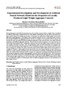
Figure 3 shows, for different values of the integrator gain KI, the dynamic responses of a single-area system
2In the per umt (pu) system,varxablesare scaledby theirnominal value and becomethereby&menslonless
186
F BeauJays, Y Abdel-Magtd, and B Wldrow
005
//•
K~- 0 3 2
/
0 ~ -0.05
-
g ~ -o.15
Kj-O04
~" -o2 ~" °0.~
-0.35
i
i
~
i
i
I
r
50
100
150
200
250
300
350
400
time (100 ~terattons - 2 5 s e c o n d s )
FIGURE 3. Dynamic responses of a conventional single-area system subject to a 10% step-load perturbation, for different values of the integrator gain.
subject to a 10% step-load increase. With no integral control ( K / = 0), the frequency fluctuations A f ( n Ts) converge to some non-zero steady-state value. To achieve zero steady-state error, the integrator must have a strictly positive gain. The higher the gain, the faster the convergence will be, but high gains tend to produce ringing in the step response, and this should be avoided for stability reasons. In practice, K, will be chosen to be the crmcal gam, that is, the highest gain that yields no overshoot (KI = 0.2 in Figure 3).
2.2. Automatic Load-Frequency Control in Two-Area Systems A two-area system consists of two single-area systems connected through a power line called the tle-hne" each area feeds its user pool, and the tie-line allows electric power to flow between the areas. Because both areas are tied together, a load perturbation in one area affects the output frequencies of both areas as well as the power flow on the tie-line. For the same reason, the control system of each area needs information about the transtunt situation in both areas to bring the local frequency back to its steady-state value. Information about the local area is found in the output frequency fluctuation of that area. Information about the other area is found
--
TIe-LI
i
--
E]ectnc Bus 1 T. . . . . . . . . . .
'
¢
~ "
[ [.
Tie-Line
t Electric Bus 2 Sensor
FIGURE 4. ConvenUonal two-area system: basic block diagram.
in the tie-hne power fluctuations. Therefore, the tieline power xs sensed, and the resulting tie-line power signal is fed back into both areas. This basic scheme is illustrated in Figure 4. A more complete diagram is given in Figure 5. One recognizes the two single-area block diagrams (dashed boxes) and the tie-line. A few additional elements are introduced whose function is next described. In steady-state, each area outputs a frequency of 60 Hz. A load perturbation occurring in either area affects the frequencies in both areas as well as the tie-line power flow. In fact, it can be shown (Elgerd, 1982) that, with small signal approximation, the fluctuation in power exchanged on the tin-line, Ap].2(t), is proportional to the d~fference between the instantaneous shaft angle variations in both areas, AO](t) and A02(t) (Elgerd, 1982). These shaft angle variations are equal to 2re times the integral of the corresponding frequency variations, Af] (t) and Af2(t). In the Laplace domain, API,2(a ) = TO[ ',-X01(s') - A 0 2 ( s ) ]
27rT o -[~F,(s) - kF2(s)],
(6)
where T Ois a constant called the tie-line synchronizing coefficient (typmally 0.0707 M W / r a d ) . This operation is illustrated in Figure 5 (right-hand part of the tieline). If, for example, the electric load increases m area 2 (APE.2(s) > 0), the frequency in area 2 decreases (AFz(s) < 0), and more power is transmitted from area 1 to area 2 [ API,2 > 0, which is in accord with eqn (6)]. In area 1, this increase in tie-line power is perceived exactly the same way as an increase in power demand from the users of area 1, that is, an increase of 6p in PI.2(s) or an increase of 6p in PE.I(s) has the same effect on the frequency FI (s). Therefore, in our model, APL,2(S) should be added to the same node as APE.~, and with the same sign (which is a minus sign ). By symmetry, AP2,~ = - AP~,2, the power going from area 2 to area 1, is added to the same node as APE,> also with a minus sign. Let us now examine how two-area systems are controlled. In conventional systems, the turbine reference power of each area is set by an integral controller. Because a perturbation in either area affects the frequency in both areas and a perturbation in one area is perceived by the other through a change in tie-hne power, the controller of each area should take as input not only the local frequency variations, but also the tie-line power variations. Because an integral controller has just one input, these two contributions (local frequency variation and tie-line power variation) must be combined into a single signal that can be inputted in the controller. The easiest way of doing this is to combine them linearly, that is, the input of the integrator in area 1 is API,2 + B~ AFt, and the input of the integrator in
Apphcatton of NN to PowerSystems Control
-1 [] LI
187
r-~
ElectricLoad
I,__1 I R' I
~.~,°.,o. "P~,,(')
T~e-Lme Power Flow Stgna.l~
I -" I T
I I
Tie-LinePowerFlow / S1gna.l /
Area 1
L.,
'
APL2(s)
,"
EL.,
Are~ 2
[ /~2 I ~
ElectricLoad
F1uctua,tlon
,
FIGURE 5. Conventional two-area system: small signal model, simplified block diagram.
area 2 is AP2,1 + B2z2kF2(see Figure 5). The coefficients BI, B2 are usually set to 1/Ke + 1/R (see Elgerd, 1982, for more details). With the orders of magnitude previously mentioned, B1 = B2 = 0.425 pu M W / H z . Following the same procedure as in the one-area case, we derive the discrete-state space equations of a two-area system. Assume for sake of simplicity that the hydraulic amplifier and turbine time constants are negligible compared to the generator time constants. Choose as discrete state variables the frequency in area 1, Af~(nTs), the frequency in area 2, Af2(nTs), and the tie-line power, Apl,2(nTs). The equations are:
Af~(nT,
+ T,) = Af~(nTs) + ~
Ke.tAp~f.l(nTs)
_ '(Ke:+IR, )Afl(nTs)- Ke,lAPE,l(nTs)] , Af2(nTs + Ts) = Af2(nTs) + ~
(7)
Ke.2Ap,~f.2(nT,)
-\(Ke'2+IR2 ) A f2(nTs)- Ke.2Ape.2(nTs)] , Apl.2(nTs + Ts) Apl.2(nTs) + Ts[2¢T°(AA(nTs)-
(8)
=
aA(nTs))].
(9)
Once again, Ts is the sampling rate. For large systems ( ~ 1000 MW), typical parameter values are: for the generator gains, Ke: = Ke,2 = 120 H z / p u MW; for the generator time constants, Te: = Te,2 = 20 s; for the regulation parameters, Rt = R2 = 2.4 H z / p u MW. For any nonnegative integrator gains K1.1,/(1,2, when a step-load perturbation has occurred in area 1 and/ or in area 2, and after transients have died out, the frequency variations in both areas converge to zero,
and so does the tie-line power [see eqn (6)]. The plant state vector x(nTs) = [Afl(nTs) Af2(nTs) Apl.E(nTs)] r converges thus to a steady-state value equal to: Xsteady.stat¢ = [ 0 0 0 ] r.
(10)
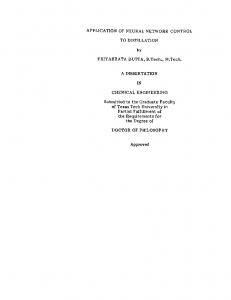
Figure 6 shows the dynamic response of a conventional two-area system subject to a 10% step-load increase in area 2. Figure 6A shows the frequency transients in both areas and Figure 6B shows the tie-line power transients. We may observe here that zero integrator gains (dashed lines) yield non-zero steady-state errors, while positive integrator gains (plain lines) do achieve convergence of the state variables to zero. In this specific plot, the gains were chosen equal to the critical gains (KI,1 = KI,2 = Kcntlcal ~--- 0 . 0 5 ) , which ensured the fastest transient recovery with no overshoot in the step response. Before leaving our discussion of conventional control systems and beginning a development of neural controls, we make an important remark. As explained in Section 2.1, the plant models used so far were linearized models. We were assuming that the operating point of the plant did not change much when a step-load perturbation occurred on the bus, and that, therefore, all the plant parameters could be kept constant. In practice though, the constant characterizing the speed regulator R depends in a highly nonlinear way upon the turbine power Pr, and this occurs as well in a single-area system as in each area of a two-area system (Cohn, 1986). The presence of this nonlinearity and the slowness of traditional integral controllers is what motivates our substituting a neural network controller for the integrator(s). To emphasize the difference in plant dy-
188 A ~-0 ~
F Beaufays. Y Abdel-Magld, and B Wtdrow
....
o
handling system nonlinearities suggested thmr substitution by nonlinear neural network controllers. A natural cho;ce of neural network architecture for a dynamic controller is the feedforward multilayer structure. Such an architecture can be adapted with the back propagation-through-time algorithm (Nguyen & Widrow, 1989, 1990; Werbos, 1990), an extension of the well-known back propagation algorithm (Werbos, 1974; Rumelhart & McClelland, 1986). Let us first briefly summarize the back propagation algorithm.
KI, 1 = KI, 2 = 0
04 -0.06
g -oos g -or ,,
N"N
-0 12
':-"--::: . . . . . . . . . . . . . . . . . . . . . . . . . . . . . . . . . . . . . . . . . . . . . . . . . . . . .
o,, -O 18
0
20
40
60
80
100
120
140
time {10 iterations - 1 second)
B
/-',,(
.... ,
o.
004
--
' K, l = KI,2 = K ~ t ~ l = 0 05
;
3.1.1. Back Propagatzon Algorzthm A feedforward multilayer neural network is shown in Figure 8A. A single neuron extracted from t h e / t h layer of a L-layer neural network is represented in Figure 8B. The inputs _vl are multiplied by the adaptive weights w~j; the output xl +l is obtained by passing the sum of the weighted inputs through a sigmoidal function s~(. ) (i.e., hyperbolic tangent) .'~~
0 03
~, j .~~
1 1)
0 02
A
O; -....
0H 0
20
I 40
m 60
f gO
100
I 120
f r e q u e n c y variation in area 1 f r e q u e n c y variation in area 2
I 140
twae (10 iterations = I second)
FIGURE 6. Dynamic response of a two-area system subject to a 10% step-lead increase in area 2. (A) Frequency transients in both areas. (B)Tie-line power transients.
*0 2
-0 25
namms for various values of the regulation parameter R, we plotted in Figure 7 the step responses of an uncontrolled two-area system (integrator gains equal to zero) for two different values of R (chosen within a reasonable physical range). Figure 7A shows the frequency transients in both areas when a 10% step perturbation hits area 2 of a system having as regulation parameters R, = R2 = 2.4 H z / p u MW. Figure 7B shows the frequency transients for a system having R~ = R~ = 6.0 H z / p u MW. Apart from the fact that the steadystate frequencies are different for different values of R, we notice that a higher regulation parameter creates more ringing in the system: the fact that R is not a constant profoundly affects the dynamic response of both generators.
-0 3 t 20
-0 35
i 40
610
80
I~lO
120
140
time ( | 0 iterations = I second)
B
0
I
1
--
frequency variation in area 1
-0 05
-0 I =o
-0 2
-0 25
~ -03
3. N O N L I N E A R C O N T R O L BY M E A N S O F NEURAL N E T W O R K S 3.1. Neural N e t w o r k Control o f a Single-Area System
We have seen in the previous section that the slowness and lack of efficiency of conventional controllers in
-0 35
0
~'o
go
60 '
80 '
1 ~o
120 '
140 '
time (10 iterations = 1 second)
FIGURE 7. Dynamic response of an uncontrolled two-area system subject to a 10% step-load increase in area 2, for different values of R. (A) R, = R2 = 2.4 Hz/pu MW. (B) R1 = R2 = 6.0 Hz/pu MW.
Applicatton of NN to Power Systems Control
189 B l ~1
I Wl,j
w~,,
FIGURE 8. Feedforward multilayer neural network. (A) L-layer neural network. (B)jth neuron extracted from the Ith layer.
Initially set to small random values, the weights are adjusted after each presentation of a new input pattern. The adaptation rule is given by: d(ere) a w l = - ~ dw~---7
(12)
where w~.j is the weight connecting neuron z in layer l with neuron j in the next layer, # is the learning rate, e is the error vector, that is, the difference between the actual and desired outputs. It can easily be shown (see Rumelhart & McClelland, 1986; Widrow & Lehr, 1990, for a detailed derivation) that eqn (12) is equivalent tO:
Aw~,j = - U6~+'. x~
(13)
where x~ is the output of neuron i in layer l. The error gradients ~j in a L-layer network are evaluated with the following recursive formula:
6~ =
{
-2ej.sj L
l = L
s'j'~
1-