ELSEVIER
Ecological Modelling 90 (1996) 39-52
Application of neural networks to modelling nonlinear relationships in ecology Sovan Lek a,*, Marc Delacoste b Philippe Baran b, Ioannis Dimopoulos a Jacques Lauga a, St6phane Aulagnier c a UMR 9964 Equipe de Biologie Quantitative, Universit~ Paul Sabatier, 118 route de Narbonne, 31062 Toulouse, France b Laboratoire d'lng~nierie Agronomique, Equipe Ichtyologie Appliqu~e, ENSAT, 145 avenue de Muret, 31076 Toulouse, France c lnstitut de Recherche sur les Grands Mammi3~res, B.P. 27, 31326 Castanet-Tolosan, France
Received 2 November 1994; accepted 23 June 1995
Abstract Two predictive modelling principles are discussed: multiple regression (MR) and neural networks (NN). The MR principle of linear modelling often gives low performance when relationships between variables are nonlinear; this is often the case in ecology; some variables must therefore be transformed. Despite these manipulations, the results often remain disappointing: poor prediction, dependence of residuals on the variable to predict. On the other hand NN are nonlinear type models. They do not necessitate transformation of variables and can give better results. The application of these two techniques to a set of ecological data (study of the relationship between density of brown trout spawning sites (redds) and habitat characteristics), shows that NN are clearly more performant than MR ( R E = 0.96 v s R 2 = 0.47 o r R E = 0.72 in raw variables or nonlinear transformed variables). With the calculation power now currently available, NN are easy to implement and can thus be recommended for modelling of a number ecological processes. Keywords: Model comparison; Multiple regression; Neural networks; Nonlinear relationships; Trout
1. Introduction For a number of years, the growing use of the aquatic ecosystem has forced the administration to address important economic and ecological problems. Habitat models, either deterministic or stochastic, based on the relationships between environment variables and characteristics of fish populations (density and biomass, reproduction potential, growth, etc.) are excellent tools for the managers. Faush et
* Corresponding author. E-mail:
[email protected]; Fax: (+33-61) 556196.
al. (1988) counted 95 models of this type. Of these 95 models published between 1950 and 1985, 79 were constructed from linear or multiple linear regression or correlation. This procedure assumes a linear relationship between the variables, which is rather rare in ecology. Then, 11 were curvilinear functions (exponential or power), and 5 were polynomial functions (but these were built up with very few variables and observations). Since this review, linear models have still been generally used (Milner et al., 1985; Jowett, 1990; etc.). On the other hand, artificial neural network (NN) systems are known for their capacity to process
0304-3800/96/$15.00 Copyright © 1996 Elsevier Science B.V. All rights reserved. SSDI 0304-3800(95)00142-5
40
S. Lek et al. / Ecological Modelling 90 (1996) 39-52
nonlinear relationships (Homik et al., 1989; Chen et al., 1990), especially for regressions (Specht, 1991). Their performance has already been demonstrated in various areas, notably in physics and economics (Nicolas et al., 1989; Waibel et al., 1989; Narendra and Parthasarathy, 1990; Sch~Sneburg, 1990; Refenes et al., 1993; Chakraborty et al., 1992; Hoptroff, 1993). In biology, works have especially been done in the medical area (Zhu et al., 1990; Blazek et al., 1991; Bazoon et al., 1994; Belenky et al., 1994; Lerner, 1994) and can be very useful for ecological process modelling. In this work, we compare the predictive capacity of multiple regression (MR) versus NN for the estimation of the density of brown trout redds from physical habitat variables in 6 mountain streams in SW France. Model-predicted and observed values are compared by different statistical parameters. Norreality and correlation of the residuals are studied.
2. Materials and methods
Twenty nine stations distributed on 6 rivers were subdivided into 205 morphodynamic units. Each unit corresponds to a zone where depth, current and gradient are homogeneous (Malavoi, 1989). The physical characteristics of the 205 morphodynamic units were measured in January, immediately after the brown trout reproduction period. They therefore most faithfully indicate the conditions met by the trout during its reproduction. With reference to the works of Ottaway et al. (1981), Shirvell and Dungey (1983), Crisp and Carling (1989), we measured 10 physical habitat variables (Table 1). 2. I. Preparation of data
i: independent, d: dependent; these independent variables are non-correlatedexceptSV and BV, R = 0.76.
and ~" and orx the mean and standard deviation of the variable. To compare the two methods (MR and NN), we worked with non-transformed variables (raw data) and also with transformed variables (requirement of MR). We proceeded to nonlinear transformations (functions of power). For each independent variable, several combinations were tested, the function that gave the best correlation with the dependent variable was retained (Delacoste, 1995). The dependent variable was also centered and reduced and nonlinearly transformed for MR, or converted over the interval [0... 1] to adapt to the transfer function used (sigmoid function) for the NN. 2.2. Multiple regression
Input data had very different orders of magnitude according to the variables. To standardize the scales of measurement, the entries were converted into centered reduced variables by the relationship: Xc Zs = ~ o-x
Table 1 Habitat variables measured to study brown trout reproduction (from Delacosteet al., 1993) Variable Type Characteristics Wi i Wettedwidth(m2) ASSG i Area with suitable spawninggravel for troutper linear meterof river (m2/linear meter) SV i Surfacevelocity(m/s) GRA i Water gradient(%) FWi i Flow/width (m3/s/m) D i Mean depth(m) SDD i Standarddeviationof depth (m) BV i Bottomvelocity(m/s) SDBV i Standard deviation of bottomvelocity(m/s) VD i Mean speed/mean depth(m/s/m) R/M d Densityof trout redds per linear meter of streambed(redds/m)
(1)
with Zs: standardized values, Xc: original values,
The technique of stepwise multiple regression (Weisberg, 1980; Tomassone et al., 1983) was used. We also undertook MR with all the variables (for further comparison with NN). Calculations were done using SYSTAT ® software (SYSTAT, 1992). As a check, optimal nonlinear transformations was also tried on the same data set, using SAS's Transreg procedure (SAS Institute, 1988). This procedure
S. Lek et al. / Ecological Modelling 90 (1996) 39-52
41
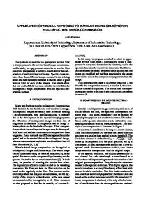
The input layer comprises n neurons coding the n pieces of information (Xl ... X,) at the entry to the system. The number of neurons in the hidden layer is chosen by the user according to the desired reliability of the results. Finally, the output layer comprises a single neuron corresponding to the value to be predicted. To each connection between two successive layers of neurons, a modifiable weight is associated in the course of the training (successive iterations) depending on the data at the entry and exit. Although the states of the neurons of the input layer are determined by the variables at the entry of the network, the other neurons (of the hidden and output layers) must evaluate the intensity of the stimulation from the neurons of the preceding layer using the following relationship: F1
F2
F3
1
aj = Y'~ XiWii
(2)
Fig. 1. Structure of the neural network used in this study. FI: input layer of neurons comprising as many neurons as variables at the entry of the system; F2: hidden layer of neurons whose number is determined empiricaly; F3: output layer of neurons with a single neuron corresponding to the single dependent variable.
with aj: activation of the jth downstream neuron, Xi: value at the outlet of the ith neuron of the
seeks an optimal transformation of variables, using the method of alternating least squares, to fit the data to a linear regression (Young, 1981; Breiman and Friedman, 1985; SAS Institute, 1988).
previous layer, W/j: weight of the connection between the ith neuron of the previous layer and the jth neuron of the current layer. With the backpropagation technique, the response of the neurons is often quantified by a sigmoid function:
i=1
2.3. Neural networks We propose here a modelling method based on one of the principles of the neural networks: the backpropagation algorithm (Rumelhart et al., 1986; Gallant, 1993). It concerns a mathematical modelling principle built on the mode of human neuron operation with a nonlinear function that transforms the activation into a prescribed reply (a short algorithm of backpropagation is presented in the Appendix). A backpropagation system typically comprises three types of neuron layers: an input layer, one or several hidden layers and an output layer comprising one or several neurons. All neurons of a given layer, except those of the last, emit an axon to each neuron of the downstream layer. In most cases only one hidden layer is used (Fig. 1) to limit the calculation time and especially when the results are satisfactory.
f(aj) = 1 + e x p ( - a j )
(3)
The backpropagation technique is akin to supervised training (to learn, the system has to know the reply that it should have given). It then modifies the connection intensity to minimize the error of the considered reply. The estimation of the error signal differs according to the layer considered. Many articles, notably Rumelhart et al. (1986), Carpenter (1989), Weigend et al. (1992) and Gallant (1993), give the details of the algorithm of error backpropagation. Lastly, note that one can use parameters such as "q (learning rate) and ot (momentum), that serve to accelerate training while preventing the system from falling into local minima (references quoted above). The training of the network continues until mini-
S. Lek et al. / Ecological Modelling 90 (1996) 39-52
42
mization of the sum of the squares of errors (SSE) given by the relationship: N
SSE = ~1 E ( Y - I~) 2 j=l
(4)
with Y: value expected at the outlet of the network ("observed" value); I~: value calculated by the network (neuron of the output layer); j = 1... N: number of recordings. NN are progressive training models which learn with the different iterations.
variable to be investigated and the average of the dependent variable ( R / M ) obtained by systematic scanning of the possible values of the other variables. In order to limit the computation time, the scanning of each variable was restricted to five levels (maximum, minimum, median and quartiles) and the number of points for each curve was limited to 12, delimiting 11 equal intervals over the variable range.
3. Fitting the models
2.4. Modelling technique 3.1. Multiple linear regression modelling Modelling was carried out in two steps: • First, fitting the models: all the records available in the set of data (i.e. 205) were used to perform the MR and to train the NN. • Secondly, testing the models: random selection was used in order to isolate a training set ( 3 / 4 of the records, i.e. 154) and an independent test set ( 1 / 4 of the records, i.e. 51). This operation was repeated five times giving rise to "test1", "test2", "test3", "test4" and "test5" which we studied by MR and by NN. For each of the five sets, the model was first adjusted with the training set (all the transformed variables for the linear MR and all the non-transformed variables for NN), and then tested with the test set.
2.5. Performance indices To judge the quality of the results obtained in MR and in NN, three indicators were used: • the correlation coefficient R between observed and estimated values, or the determination coefficient R2; • The slope of the regression between values estimated by models and observed values; • the study of residuals: E,. = 1I/- I~/, their statistical parameters, graphs of normality, etc.
2.6. NN sensitivity For the NN, any analytic study of model sensitivity seems difficult. However, one can obtain a curve illustrating this effect plotting fixed values of the
3.1.1. Stepwise model Whether the variables were transformed or not, only four independent variables were retained by the model. Three of the four variables were common to the two models: ASSG, GRA and D (see Table 1). The fourth independent variable concerns Wi which was retained for the model with transformed variables and SV for the model with non-transformed variables. Equations of MR and the determination coefficients were the following: - With transformations of variables: R 2 = 0.622
1 ~ R / M = 2.292 + 1.282~-~1 - 2.933
1 ASS--~
1 - 0 . 0 9 1 GfG--ffA+ 10.605-D
(5)
- Without transformation of variables: R 2 = 0.444 R / M = 1.051 + 0.459ASSG - 0.403SV - 0.054GRA - 0.012D
(6)
Values of the determination coefficient indicate a plain improvement of the MR model after transformation of the variables. As this operation improves their linearity, we can conclude that nonlinear relationships exist between the dependent and independent variables.
3.1.2. Complete model With all the 10 variables, equations of MR and determination coefficients became:
S. Lek et al. /Ecological Modelling 90 (1996) 39-52
30
43
O
4-
20
[-, 10
0
3
c~
2.
~
0
0
-10
-1 0
5
10
15
oOc~ O
1. ',
20
2.5
5 ASSG
wi
7.5
10
16
1.5
O
> r~
[-
'r 8
0.5
4
0
I
-0.5
O I
I
10
15
-4
0
1
2
0
sv 1
5
20
GILA
140 120 100
0 0
°~
O
0
0.6
~
O
so
0.4 0. I
0
0.2
0.4
0.6
}
I
25
50
75
D
FWi
25
120
oa~O
15 10 5 0 -5 -10
O 8O
0
4o 20
I
-20 0
10
20 SDD
30
40
0
25
50
75
BV
30
6
c~
20
4 3 2 I
0
1
0 -1
-lO 25
50 SDBV
75
I
i
2.5
5
O
7.5
VD
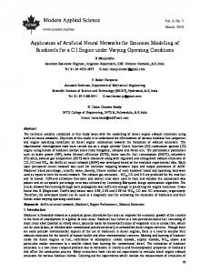
Fig. 2. Nonlinear transformation of variables by the Transreg procedure of SAS. For each of the 10 independent variables, both the raw value (in abscissa) and the transformed value (beginning with T, in ordinate) are plotted.
44
S. Lek et al. / Ecological Modelling 90 (1996) 39-52 40
- with transformations of variables: R 2 = 0.63 1
1
30
1/-R--/M = 2.517 + 0 981 ~-~ - 2.852 ASSG
o25
- 0.372 SvrSV - 0 . 0 4 9 ~ 1
+ 0.194~
+ 8.434-D
m 5 ......
1
+ 0.509
SDD
i
10
+ 0.005BV
- 0.005SDBV - 0.004VD
R / M = 1.337 - 0.019Wi + 0.479ASSG - 0.570SV - 0.047GRA + 1.309FWi - 0.013D - 0.008SOD + 0.010BV - 0.014SDBV - o.018vD
1000
1.0
(7)
- without transformation of variables: R z = 0.469
• 100
.~ 0.8
~
0.6
g o.4 0.2 "~0.0
(8)
As during the stepwise regression, the transformation of variables gives rise to a clear improvement of the determination coefficient. By including all independent variables in the model, there is only a very slight increase of R 2. Supplementary variables (SV, FWi, VD, BV, SDBV) bring little complementary
~-0.2 -0.4
i
ll,ll 10
i i ,llll 100
1000
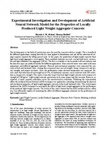
Number of Iterations Fig. 4. Neural network modelling: variation of the sum squared of errors and the correlation coefficient between observed and estimated values according to the number of iterations.
information. Among the regression coefficients calculated with all the variables, only three were significantly different from 0: ASSG, Wi and D for the transformed variables and ASSG, GRA and SV for the non-transformed variables (variables selected in the stepwise regression).
0.95
0,9
o ~
0.85
0.S
0.75 5
10
15
Number of Hidden Units Fig. 3. Neural network modelling: variation of the correlation coefficient between observed and estimated values according to the number of neurons of the hidden layer (average value and standard deviation).
3.1.3. Optimal nonlinear transformation of variables Since most of the relationships between the variables appear to be nonlinear, a method of alternating least squares was used. After 30 iterations of Transreg procedure the optimal transformations were finally derived, yielding a determination coefficient R 2 = 0.72, higher than in the linear case (R 2 = 0.469). Fig. 2 depicts the various transformations imposed on the data set. Interpreting such transformations is debatable: the improvement in R 2 is here obtained at the expense of warping the data under study in a non-meaningful manner. Rather than linearily combining transformed variates, the NN approach will combines the raw data in a nonlinear model.
S. Lek et al. // Ecological Modelling 90 (1996) 39-52
3.2. Remarks on NN modelling To avoid overfitting (noise modelling; Smith, 1994), we took two factors into account: the number of neurons in the hidden layer and the stopping point of the training. 3.2.1. Number of hidden layer neurons For statistical modelling, only one hidden layer is often satisfactory (Smith, 1994). We therefore studied here the performance of the model with a system
2.5 -~
45
with one hidden layer, by varying the number of neurons. For each configuration, the experiment was repeated 5 times, and each time we calculated the correlation coefficient between the estimated and observed values of the dependent variable. We trained NN with all the non-transformed variables which gives the best result. Fig. 3 shows the values obtained and the average value curve. We first observe a rapid improvement of R with the number of neurons in the hidden layer (HN). The increase is then slower and stabilizes from 8 hidden neurons.
I!
b
4
o
/I
//
vl
~ "~ •~
3
1.5
2
1
1
0.5 0
0
. . . . . . . . . . . . . . . . . .
-0.5 -0.5
0.5
~ 2.5
1.5
-1 -I
Observed values
1
2
3
-
2 1.5
•
4
Observed values
41
2.5
"~
0
,///I
1
'N 0.5
°
O-
0 -0.5 -0.5
0
0.5
1
, 1.5
-1 2
2.5
~--1
0
Observed values
1
I
% - - 42
3
~
i 4
Observed values
2.5--
4F
2 1.5
~
3
•~
2
.~ 0.5
,
l
r~
~
o
~
0
...........
-0.5 -0.5
0
0.5
1
1.5
Observed values
2
2.5
-1
0
1
2
3
4
Observed values
Fig. 5. Correlation graphs between observed and estimated values of R / M by different models: (a) multiple regression (MR) with transformed variables; (b) multiple regression (MR) with non-transformed variables; (c) neural network with four independent variables (NN4) with transformed variables; (d) neural network with four independent variables (NN4) with non-transformed variables; (e) neural network with all the independent variables (NNT) with transformed variables; (f) neural network with all the independent variables (NNT) with non-transformed variables.
46
S. Lek et al. / Ecological Modelling 90 (1996) 39-52
For a given value of HN, the correlation coefficients obtained were similar, proof of the reliability of the NN results. Maximum divergence was observed when HN = 2, the standard deviation of R was then 0.008, largely exceeding the average value of 0.004. Therefore all our models were run with 8 neurons in the hidden layer, a choice that is justified by the absence of improvement of the performance of the model beyond this value and a relatively small standard deviation.
3.2.2. The stopping point of training In NN, the stopping point of training must be fixed, i.e. the number of iterations calculated by the system. We studied the sum of the squares of errors (SSE) and the correlation coefficient (R) for all the non-transformed variables. At each iteration, the system corrects weights to minimize error. Thus, as the system learns, the SSE decreases (Fig. 4a), while coefficient R increases (Fig. 4b); the convergence of the model is very fast. At the end of some hundreds of iterations, the SSE is practically nil, while R approaches 1. The result stabilizes after 1000 iterations. 3.3. Neural networks modelling In order to compare the results of the NN with those of MR, we established NN models with the four independent variables selected by the stepwise MR, but also with all the available variables.
3.3.1. With four variables selected by the stepwise regression • transformed variables: after 1000 iterations, we obtained a model with a determination coefficient R 2 = 0.741, which indicates a slight improvement with respect to MR. • non-transformed variables: after the same number of iterations, the determination coefficient became R 2 = 0.811. Compared to the model obtained with transformed variables, and unlike for MR, an improvement was observed with raw data. The transformation of variables giving the best linearity of relationships between variables therefore led to a lowering of NN type nonlinear model performance.
3.3.2. With all the variables transformed variables: R 2 = 0.928 non-transformed variables: R 2 = 0.958 Unlike MR models, a clear improvement of the results was obtained by including additional variables. The results were improved with the transformed variables as well as with the non-transformed variables. The additional variables do bring specific information. As in the case of the model with four independent variables, a better result was obtained with non-transformed variables.
4. Performance of the models
4.1. Correlation between observed and estimated values In MR, the transformation of variables significantly improves the determination coefficient ( R 2 = 0.643 vs R 2 = 0.444). There is, however, an underestimation of the high values and an overestimation of the low values (Fig. 5a and b). We can also see the difficulty for the MR model to predict nil values indicated on the graph by a vertical band. We can finally note the negative value prediction, especially for low values. In NN with four explanatory variables (NN4), we obtained an underestimation of high values. As with MR, the model has difficulties to predict nil values, but only with transformed variables (Fig. 5c). With non-transformed variables, adjustment is better, especially for low values (Fig. 5d). In NN with all the available variables (NNT), the problem remains with transformed variables for nil values, as well as for some low values (Fig. 5e). With non-transformed variables, however, an excellent model was Obtained capable of restoring values observed over the whole range of the dependent variable (Fig. 5f). Note finally that NN, unlike MR, never predicted negative values. The regression between values estimated by the different models and observed values (Table 2) revealed that the slope (b) with a value closest to 1 was obtained for the neural network with all the non-transformed variables (NNT) ( b - - 1 , reduced standard deviation and Student's t test close to 1.96). On the other hand, in MR the results were
47
S. Lek et al. / Ecological Modelling 90 (1996) 39-52
Table 2 Slopes (b) of regression between estimated and observed value for multiple regression (MR) and neural networks (NN) models Transformation of data
Model
Slope (b)
Standard deviation (sb)
t test
Yes Yes Yes No No No
MR4 NN4 NNT MR4 NN4 NNT
0.643 0.681 0.844 0.463 0.774 0.968
0.034 0.028 0.023 0.035 0.026 0.014
10.50 11.39 6.78 15.34 8.69 2.29
much poorer, especially with non-transformed variables ( b - - 0 . 4 6 , standard deviation and Student's t test high). In conclusion, to obtain the best models, all the variables must be used without tranformation for the neural network system.
4.2. Examination of the residuals
MR4: MR with four independent variables; NN4: NN with four independent variables; and NNT: NN with all the independent variables. t: Student's t test for H0: b = 1.
4.2.1. Normality of the residuals To test the normality of model residuals, we
applied the statistical test of Lilliefors (1967). With 205 observations, limit values of the test for the
b
a 0.25
e~
0.20
30
0.15
-
~~~,.c~
-40
0.15
20 ~o
0.i0
O
O
lO
0.05
0.i0
!
50
~\
30
0
-20
~
10
0.05 rl
-I.00
-0.30
0.40
1.10
-I,60
Residual 0.50
0.20"
40
0.15
30
O O
'J~
(3
0.i0
20
0 "~
O. 0 5
I0
0
,
-0.60
r
,
0.10
0.80
100
0.40
80
C~
0.30
60
0.20
40
0.10
L20 ,
1.50
0
-0.00
,
P
0.60
2.00
3,40
Residual
I
e
f 40
~'~
2.60
d
Residual
.~
1.20
Residual
c
t2
-0.20
O, 15
30
0.10
20
0-05 i
10
0 , 4 0
e~
EO
80
70
0.30
60 50
0.20
40
0.10
3O "20 10
C~
~0
"
-0.40
-0.05
0.30
Residual
0.65
-0.50
0.20
0.90
1.60
Residual
Fig. 6. Distribution of residuals (observed values - estimated values of R/M) with adjustment to the normal law for the different models: (a) MR, transformed variables; (b) MR, non-transformed variables; (c) NN4, transformed variables; (d) NN4, non-transformed variables; (e) NNT, transformed variables; (f) NNT, non-transformed variables.
S. Lek et al. /Ecological Modelling 90 (1996) 39-52
48
Table 3 Results of the Lilliefors (1967) test of residual normality for the different models Transformation
Model
MaxDif
Prob (2-tail)
Yes Yes Yes
MR NN4 NNT MR NN4 NNT
0.028 0.075 0.061 0.127 0.136 0.077
1.000 0.007 0.063
No No No
0.000 0.000 0.005
MaxDif: maximum value of the difference; Prob (2-tail): probability limits. MR4, NN4 and NNT: see Table 2.
rejection of the hypothesis of normality were 0.062 for ot = 0.05 and 0.072 for ot -- 0.01. The results (Table 3) show that the transformation of variables gives models whose residuals are normaly distributed. This is the case with the MR and NNT. For the NN4, the residual distribution is not
l |
--o-
II
/
J.
4.2.2. Relationship between residuals and the dependent variable With transformed variables, residuals are independent of estimated values for all models (Fig. 7a, c and e) and of observed values in NNT (Fig. 70. In MR and NN4, residuals tend to increase with observed values (Fig. 7b and d). It can be noted that, in all cases, there are some dots corresponding to nil
it
°
bl
o.5 Jr
~^~.._~o Oo ,~ _ . o ~ oo o
e ~_°o_.o o o ~ o,,gl.J~ hS~'/~-,~ o~o o
0.5 ~-
far from normality for ot = 0.01. Fig. 6a, c and e show the distribution of the residuals under the normal curve. On the other hand, for non-transformed variables, the residual distribution was very far from normality for the MR and NN4 models. The graphs show many deviations f r o m normality for MR and NN4 (Fig. 610 and d). NNT however showed an appreciably normal distribution of residuals with a 1% risk. The graph (Fig. 6f), which is better balanced, reveals the presence of some strong values that detract from the normality of the residuals.
............ o.
I I
........o . . . . . . .
I
°o
~ -0.5
-11 -0.5
i
t
)
?
0
0.5
1
1.5
-1 4-
i°
L
I
I
0
0.5
1
1.5
2
Observed values
Estimated values
o.T o°ooot 1|
°°
2.5
o
c~
.............
. . . .
1
o o
d
0.5 0 -0.5
-0.5.1 l -0.5
0
I
q
i
!
0.5
1
1.5
-1 2
0.5
0
I
I
I
1
1.5
2
2.5
Observed values
Estimated values 1 i .~
b 0.5
1
f
i o o o Oo . . . . . . . . . o-
..................
-0.5 -1
-0.5
0
I
I
i
0.5
1
1.5
Estimated values
0
0.5
1
1.5
2
2.5
Observed values
Fig. 7. Relationship between the residuals and the estimated and observed values of R / M for transformed variable models: a, b: MR; c, d; NN4; e, f: NNT.
S. Lek et al. / Ecological Modelling 90 (1996) 39-52 2A-
o
/
%0
o
o
2
II
"~
0
¢~
-1
o
o
-2/ -I
0
i
°1
l
2
i°
-2
3
4
I
2
o ! 0
o
C t:P
O •
1
O
............. ...............
o
0 ......
4
5
o
!og
0
d1
O
~b
o........
o
J i
-1
-1 -2 ] -1
l 0
I 1
I 2
I 3
--q 4
-2 0
1
2
2t 1
0
e
~o
..............
3
4
5
Observed values
Estimated values
o
3
Observed values
Estimated values
o
49
f 1
o
~ °
~o
80.oO% o
-I + -1
0
1
2
0
3
Estimated values
1
2
3
4
Observed values
Fig. 8. Relationship between the residuals and the estimated and observed values of R / M for non-transformed variable models: a, b: MR; c, d: NN4; e, f: NNT.
values of the dependent variable that the model has difficulties to adjust (as mentioned above). With non-transformed variables, residuals were not independent of estimated values in MR. Moreover, a line of dots is observed in addition to some negative values (Hg. 8a). The residuals were clearly dependent on the observed values (Fig. 8b) with a significant correlation coefficient ( R = 0 . 7 3 ) . For NN, either with estimated or observed values, the dots were scattered on either side of the line of ordinate 0, i.e. the average of the residuals (Fig. 8c, d, e and f). The correlation coefficient ranged from R = - 0 . 0 4 7 to R = 0.094 for the NNT and from R = 0.158 to R = 0.517 for the NN4.
five test fractions from which they were independent (Table 4). In MR, determination coefficients were weak in two sets. R 2 was on average 0.468 for the training set and 0.371 in the test set. In NN, the
Table 4 Results of the NN and MR models on random training set fractions ( 3 / 4 of the records) and test set fractions (the remaining 1 / 4 records) No. Test
NN
MR
R learn
R_test
R_learn
R_test
0.892 0.914 0.904 0.883 0.905 0.900
0.862 0.888 0.906 0.867 0.906 0.886
0.685 0.685 0.690 0.688 0.669 0.684
0.487 0.628 0.626 0.566 0.740 0.609
5. Testing the m o d e l s
1 2 3 4 5 Mean
The prediction power of the different models determined from five training fractions was tested on
R_learn: correlation coefficient between estimated and observed values of the training sets; R t e s t : correlation coefficient of the test sets.
S. Lek et al. / Ecological Modelling 90 (1996) 39-52
50
determination coefficient is high in the training set as well as in the test set (averages R 2 -- 0.8 and R 2 = 0.785). These results clearly demontrate the better predictive performance of NN compared to MR.
ima. Wi, SDD and BV display the same curves but with different origins and amplitudes; • constant: the contribution of the independent variable (e.g. SDBV, FWI and D) is not altered over its range. The profile is represented by a horizontal "line". Contributions therefore differ according to the independent variables considered. For each variable, a precise idea of the contribution is obtained for an interval of given value.
6. NN sensitivity Fig. 9 shows the influence of five independent variables (Wi, ASSG, GRA, SDBV and VD) on NN modelling. The 12 points cover the range of variation of each of the variables tested, with a class interval which varies according to the variable. Here five curves represent five sensitivity (or contribution) types: • inverse exponential: the low values of the independent variable, such as GRA and SV, heavily contribute to the prediction of R / M , while the high values ( > level 6) are not relevant for the model; • logarithmic: the contribution of the independent variable (e.g. ASSG) is negligible for the lowest values, but it increases quickly to reach an asymptote at early as level 4; , Gaussian: the independent variable contributes mostly around its average values (level 7). In the case of VD, this is particularly pronounced; • sinusoidal: the contribution of the independent variable run through alternative maxima and min-
7. Conclusion Either MR or NN can be used to predict the density of brown trout redds from the sampled physical habitat variables, R 2 reached 0.65 in MR (after transformation of variables), 0.72 (after maximum transformation possibility) in SAS and 0.96 in NN, the latter giving better results with non-transformed variables. In addition, the fact that NN provide a better model was highlighted by a better prediction for the low (and nil) values, the normality of the residuals and their independence from the variable to be predicted. These results were replicated and even the predictions for original test sets were more accurate with NN than MR. In ecology, MR is currently one of the most frequently used tools in predictive modelling. It is
0.7 0.6 0.5
--,*--.Wi ..""
0.4
---.-It~ VD ---o--- SDBV
,o"
- ~-- ASSG
0.30.2
/
--- A
A -GRA.
0.I 0.0
~ 0
t 2
b 4
I
~-
I
6
8
10
12
Range of the independentvariables Fig. 9. Contributionprofileof each independentvariableto the predictionof R/M by NN (five variablesare only representedhere, see text for the others).
S. Lek et al. / Ecological Modelling 90 (1996) 39-52
simple to implement if relationships between variables are linear. If they are nonlinear, a preliminary transformation is necessary. This tends to minimize nonlinearity in the process. One can equally combine variables or eliminate some to try to obtain a better predictive model. Despite all these transformations, results are sometimes non-optimum; the model often supplies negative value predictions, and the residuals are not independent from the variable to be predicted as displayed in this study. NN constitute a new and alternative approach in ecology. They are able to work with non linearly related variables. AS a matter of fact they do not set constraints on the variables (e.g. normality and/or nonlinear relationships), better still, they can be more efficient working with raw than with transformed data. With present computer power, they are also relatively easy to perform. Unlike MR, NN do not provide simple equations for users but it is possible to easily quantify the contribution of each variable over its range. Through this ichthyological example, NN can be seen to be a powerful predictive alternative in comparison to the traditional multiple regression techniques.
Appendix A. A brief algorithm of backpropagation in neural networks 1. Initialize the number of hidden nodes 2. Initialize the maximum number of iteration and the learning rate (-q). Set all weights and thresholds to small random numbers. Thresholds are weights with corresponding inputs always equal to 1. 3. For each training vector (input Xp = ( x p x 2..... xn), output Y) repeat steps 4-7. 4. Present the input vector to input nodes and the output to the output nodes; 5. Calculate the input to the hidden nodes: h
aj =
n
~
h
Wij x i
i=1
Calculate the output from the hidden nodes:
x h = f ( a h) = 1/(1 + e x p ( - - a h ) )
51
Calculate the inputs to the output nodes: L
a k = E Wjkx; j=l
and the corresponding outputs: I), = f ( a , ) =
1/(1 + e x p ( - a k ) )
Notice that k = 1 and I9k = I), L is the number of hidden nodes. 6. Calculate the error term for the output node:
6k = (Y-- Y ) f ' ( a k ) and for the hidden nodes: 6jh = f ' ( a h ) E 6kWjk k
7. Update weights on the output layer: Wjk(t + 1) = Wjk(t ) + r/akV and the hidden layer:
Wij( t + 1) -- Wij( t ) + rlajhx, While network errors are larger than some predefined limit or number of iteration is smaller than the maximum number of iterations repeat steps 4-7.
References Bazoon, M., Stacey, D.A., Cui, C. and Harauz, G., 1994. A hierarchical artificial neural network system for the classification of cortical cells. In: Proceedings of the IEEE International Conference on Neural Networks. IEEE, Orlando, FL, pp. 3525-3529. Belenky, G., Sing, H.C., Thomas, M.L., Shaham, Y., Balwinski, S., Thorne, D.R., Redmond, D.P. and Balkin, J.T., 1994. Discrimination of rested from sleep-deprived EEG in awake normal humans by artificial neural network. In: Proceedings of the IEEE International Conference on Neural Networks. IEEE, Orlando, FL, pp. 3521-3524. Blazek, M., Pancoska, P. and Keiderling, T.A., 1991. Backpropagation neural network analysis of circular dichroism spectra of globular proteins. Neurocomputing, 3: 247-257. Breiman, L. and Friedman, J.H., 1985. Estimating optimal transformations for multiple regression and correlation. J. Am. Stat. Assoc., 77: 580-619. Carpenter, G.A., 1989. Neural network models for pattern recognition and associative memory. Neural Networks, 2: 243-257. Chakraborty, K., Mehrotra, K., Mohan, C.K. and Ranka, S., 1992. Forecasting the behavior of multivariate time series using neural networks. Neural Networks, 5: 961-970.
52
S. Lek et al. / Ecological Modelling 90 (1996) 39-52
Chen, S., Billings, S.A. and Grant, P.M., 1990. Non-linear system identification using neural networks. Int. J. Control, 51:11911214.
Crisp, D.T. and Carling, P.A., 1989. Observations on sitting, dimension and structure of salmonid redds. J. Fish Biol., 34: 119-134. Delacoste, M., 1995. Analyse de la vadabilit6 spatiale de la reproduction de la truite commune (Salmo trutta L.). Etude ~t l'6chelle du micro et du macrohabitat dans 6 rivi~res des Pyr~n6es centrales. PhD. Thesis, I.N.P. Toulouse, 135 pp. Delacoste, M., Baran, P., Dauba, F. and Belaud, A., 1993. Etude du macrohabitat de reproduction de la truite commune (Salmo trutta L.) dans une rivi~re pyr6n6enne, La Neste du Louron. Evaluation d'un potentiel de l'habitat physique de reproduction. Bull. Fr. P~che Pisci., 331: 341-356. Faush, K.D., Hawkes, C.L. and Parsons, M.G., 1988. Models that predict the standing crop of stream fish from habitat variables: 1950-85. Gen. Tech. Rep. PNW-GTR-213. U.S. Department of Agriculture, Forest Service, Pacific Northwest Research Station, Portland, OR, 52 pp. Gallant, S.I., 1993. Neural Network Learning and Expert Systems. M.I.T. Press, London, 365 pp. Hoptroff, R.G., 1993. The principles and practice of time series forecasting and business modelling using neural nets. Neural Comput. Appl., 1: 59-66. Hornik, K., Stinchcombe, M. and White, H., 1989. Multilayer feedforward networks are universal approximators. Neural Networks, 2: 359-366. Jowett, I.G., 1990. Factors related to the distribution and abundance of brown and rainbow trout in New Zealand clear-water rivers. N.Z.J. Mar. Fresh. Res., 24: 429-440. Leruer B., 1994, Feature selection and chromosome classification using a multilayer perceptron neural network. In: Proceedings of the IEEE International Conference on Neural Networks. IEEE, Orlando, FL, pp. 3540-3545. Lilliefors, H.W., 1967. On the Kolmogorov-Smiruov test for normality with mean and variance unknown. J. Am. Stat. Assoc., 62: 399-402. Malavoi, J.R., 1989. Typologie des facies d'6coulement ou unit6s morpho-dynamiques d'un cours d'eau ~t haute 6nergie. Bull. Fr. PSche Pisci., 315: 189-210. Milner, N.J., Hemsworth, R.J. and Jones, B.E., 1985. Habitat evaluation as a fisheries management tool. J. Fish Biol., 27: 85-108. Narendra, K. and Parthasarathy, K., 1990. Identification and control of dynamical systems using neural networks. IEEE Trans. Neural Networks, 1: 4-27. Nicolas, J.M., Lemer, A. and Legitimus, D,, 1989. Identification
automatique de bruits impulsifs en acoustique sous-madne par r6seaux multi-couches. In: Neuro-N~mes'89, International Workshop Neural Networks and their Applications, N~mes (France), 13-16 November 1989. EC2, Nanterre, pp. 269-278. Ottaway, E.M., Carling, P.A., Clarke, A. and Reader, N.A., 1981. Observation on the structure of brown trout, Salmo trutta Linnaeus, redds. J. Fish Biol., 19: 593-607. Refenes, A.N., Azema-Barac, M., Chen, W. and Karoussos, S.A., 1993. Currency exchange rate prediction and neural network design strategies. Neural Comput. Appl., 1: 46-58. Rumelhart, D.E., Hinton, G.E. and Williams, R.J., 1986. Learning representations by back-propagating error. Nature, 323: 533536. SAS Institute, 1988. SAS Technical report P-179. Additional SAS/STAT procedures, Release 6.03, SAS Institute, Cary, NC, 255 pp. Sch~neburg, E., 1990. Stock price prediction using neural networks: a project report. Neurocomputing, 2: 17-27. Shirvell, C.S. and Dungey, R.G., 1983. Microhabitats chosen by brown trout for feeding and spawning in rivers. Trans. Am. Fish. Soc., 112: 355-367. Smith, M., 1994. Neural Networks for Statistical Modelling. Van Nostrand Reinhold, New York, 235 pp. Specht, D.F., 1991. A general regression neural network. IEEE Trans. Neural Networks, 2: 568-576. SYSTAT, 1992. Statistics, version 5.2 Edition. Systat Inc., Evanston, 724 pp. Tomassone, R., Lesquoy, E. and Miller, C., 1983. La r~gression, nouveaux regards sur une ancienne m~thode statistique. INRA (Actualit~s scientifiques et agronomiques no. 13), Paris, 177 PP. Walbel, A., Hanazawa, T., Hinton, G. Shikano, K. and Lang, K.J., 1989. Phoneme recognition using time-delay neural networks. IEEE Trans. Acoust., Speech Signal Process., 37: 328-339. Weigend, A.S., Huberman, B.A. and Rumelhart, D.E., 1992. Predicting sunspots and exchange rates with connectionist networks. In: M. Casdagli and S. Eubank (Editors), Nonlinear Modelling and Forecasting, SFI Studies in the Sciences of Complexity, Proc. Vol. XII. Addison-Wesley, Redwood City, pp. 395-432. Weisberg S., 1980. Applied Linear Regression. John Wiley, New York, 324 pp. Young, F.W., 1981. Quantitative analysis of qualitative data. Psychometrika, 46: 357-388. Zhu, K., Noakes, P.D. and Green, A,D.P., 1990. Training neural networks for ECG feature recognition. In: Proceeding of the International Neural Networks Conference, Paris, 9-13 July 1990. Kluwer, Dordrecht, pp. 137-140.