Dynamical Nonlinear Neural Networks with

International Journal of Computer Applications (0975 – 8887) Volume 85 – No 15, January 2014

Dynamical Nonlinear Neural Networks with Perturbations Modeling and Global Robust Stability Analysis Gamal A. Elnashar Automatic Control Center School of Engineering-Egyptian Armed Forces 15 Yassien Raghb St., Nasr City, Cairo, Egypt

ABSTRACT This paper is devoted to studying both the global and local stability of dynamical neural networks. In particular, it has focused on nonlinear neural networks with perturbation. Properties relating to asymptotic and exponential stability and instability have been detailed. This paper also looks at the robustness of neural networks to perturbations and examines if the related properties have been preserved. Circumstances for global and local exponential stability of nonlinear neural network dynamics have been studied. We mentioned that the local exponential stability of any equilibrium point of dynamical neural networks is equivalent to the stability of the linearized system around that equilibrium point. From this, some well-known and new sufficient conditions for local exponential stability of neural networks have been obtained. The Lyapunov’s procedure has been used to analyze the stability property of nonlinear dynamical systems and many outcomes have been combined and generalized. A kind of Lyapunov’s stability of the stable points of Hopfield neural network (HNN) have been proven, which means that if the initial state of the network is close enough to a stable point, then the network state will remain in a small neighborhood of the stable point. These stability results indicate the convergence of the memory process of HNN. The theoretical results are illustrated through a few problem cases for a nonlinear dynamical system with perturbation behavior.

Keywords Perturbed nonlinear systems, Hopfield neural network, Lyapunov stability, equilibrium state

1. INTRODUCTION It is well known that neural networks are complex and large scale nonlinear dynamical system. Dr. John Hopfield is the person perhaps most responsible for innovation of the neural network field after publication of perceptrons. His involvements include work conceptualizing neural networks in terms of an energy model. He showed that an energy function exists for the network and that processing elements with bistable outputs are guaranteed to converge to a stable local energy minimum. His presentation at the National Academy of Science meeting in 1982 triggered the subsequent large scale interest in neural networks [1]. Hopfield networks are symmetric recurrent neural networks which exhibitmotions in the state space which converge to minima of energy. Recently, the study of neural networks and applications has attracted many researchers from different disciplines. Neural networks have special nonlinear structure and method of information processing , in analogy of human being’s brain. Great success has been achieved in many different areas and may solve some difficult problems, which are difficult to be solved by conventional methods. In particular, the development of HNN has motivated a new high

rush in the study of NN. This lies in the fact that they are extremely robust to malfunctions. Their dynamic behavior exhibits stable states and this is advantageous. For example, a time evolution of an array of neuron-like elements towards equilibrium points can be viewed as the evolution of an imperfect pattern towards a correct stored pattern. This is similar to the storage of information in an associative memory [2-3] The qualitative properties of dynamical neural networks have been intensively investigated by Miche and his colleagues [4-5]. They applied large scale system techniques to obtain a large set of sufficient conditions for local asymptotic (exponential) stability for a few classes of dynamical neural networks. However, a problem normally encountered in this approach is the existence of more than one equilibrium point which may correspond to local minima. Global properties are hard to extract, and a global minimum is difficult to achieve. To overcome this dilemma, it is desirable to design neural networks which have only one unique equilibrium point and are globally stable (or attractive) so that the global property can be extracted. In this case, we do not need to specify the initial conditions of neural circuits, since all trajectories starting from anywhere will settle down to the same unique equilibrium. This equilibrium depends only on the external stimuli. In the last decade, the dynamical characteristics (including stable, unstable, oscillatory, and chaotic behavior) of Hopfield neural networks have become a subject of intense research activities. Many stability criteria are obtained. We refer the reader to [6–7] and the references cited therein. Hirsch [8 ] noted that the importance of global stability or global attractiveness and obtained a few sufficient conditions using Gershgorin’s circle theorem. Matsuoka [9 ] generalized some of Hirsch’s and Kelly[10] results using a new Lyapunov function. Yang and Dillon [11 ] also obtained some sufficient conditions for local exponential stability and for the existence and uniqueness of an equilibrium point. However, they failed to give any condition for global stability, because there exists such a system that although it has a unique equilibrium point and it is locally exponential stable, it may not be globally stable. This paper concentrates on both the global stability and local stability of Hopfield dynamical neural networks. We apply Lyapunov's methods to analyze stability of the Hopfield neural network. The neural network is viewed as a large interconnected dynamical system—that is, as an interconnection of many neurons. First we analyze stability properties of a single neuron, and then we proceed with the stability analysis of the whole network in terms of the properties of the single neurons. Interconnection information is used in union with the properties of the individual neurons to obtain satisfactory conditions for asymptotic stability of the whole network. The paper is organized as follows: In section 2, the Hopfield neural network model is described briefly. In Section 3, the stability properties of neural networks are outlines. Then, in Section 4, Hopfield neural models stability

14

International Journal of Computer Applications (0975 – 8887) Volume 85 – No 15, January 2014 analysis is summarized. In addition to robustness properties of perturbed neural networks, the stability properties of both unperturbed and perturbed neural networks are addressed and reviewed in Section 5. A numerical test illustrates some important points in Section 6.

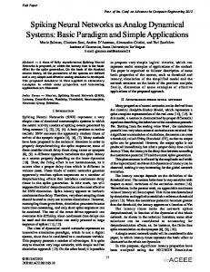
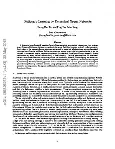
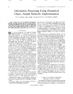
2. MATHEMATICS FOR HOPFIELD NETWORK A typical Hopfield network is shown in Figure 1. It has only one computing layer, called Hopfield layer, and the other two layers are the input and output buffers [12 ]. In terms of the backpropagtion network, the Hopfield network has feedback from each neurons to each of other neurons, but not to itself. The analog Hopfield neural network is a dynamical system whose schematic is shown in Figure 1. It is a nonlinear interconnected system proposed by Hopfield [13 ] as a model of biological neural networks. Each node, or neuron is represented by a circle. The structure of a neuron is depicted in Figure 2. The nonlinear amplifier in Figure 2 has an inputoutput characteristic described by a function g : R  [0,1] , It is commonly assumed that g is continuously differentiable and strictly monotonically increasing, that is, g(u) > g(u') if u > u'. The function g is called the activation function. A circuit implementation of the Hopfield network is shown in Figure 3. To derive equations that model the Hopfield neural network, we use an equivalent representation of the single node of the Hopfield network shown in Figure 4. Applying Kirchhoff's current law at the input of each amplifier of the equivalent node representation and taking into account that the current into the amplifier is negligibly small due to the amplifier's high input resistance, we get

Ci

du i u x u x ui  i  1 i  2  dt Ri Ri 1 Ri 2

    x  t   Tx  I  1 dg (x n )  Cn dx n  0

 g 1 (x 1 )     r1     1   g (x n )   r   n 

(5)

The operation of the Hopfield network can be best understood in terms of the energy (error) function. The wells in the energy landscape represent patterns stored in the network. An unknown pattern represents a particular point in the energy landscape and as the network iterates its way to a solution, the point is expected to move towards one of these wells. These basins of attractions represent the stable states of the network. Associated with the Hopfield neural network is its n computational energy function, E : R  R E, given by

(1)

x ui  n  I i , i  1, 2,..., n R in where x i  g (u i ). and let T ij 

 dg 1 (x 1 ) C 1 dx 1     0  

1 1 n 1 ,  T ij  . (2) R ij ri j 1 Ri

Fig 1: Hopfield neural network model

Substituting (2) into (1) yields

Ci

du i u x u x ui  i  1 i  2  dt Ri Ri 1 Ri 2

(3)

x ui  n  I i , i  1, 2,..., n R in

The system of n first-order nonlinear differential equations given by (3) constitutes a model of the Hopfield neural network. The Hopfield neural network can be viewed as an associative memory. Note that the activation function g is, by assumption, strictly increasing and differentiable. Therefore

g 1 exists and is also differentiable. We rewrite equations (3) as 1

1

dg (x i ) dx i g (x i )   T ij  I i , i  1, 2,..., n dx i dt ri j 1 Let T  R

nxn

be the matrix whose elements are

I  i 1 i 2 ...i n   R n

Fig 2: A neuron model in the HNN

n

(4)

T ij

and

T

. Using this notation, we represent

(3) in matrix form:

15

International Journal of Computer Applications (0975 – 8887) Volume 85 – No 15, January 2014

assume

that,

g (0)  0

Ci  0

and

to

u i  bi u i  Aij g j u j   U i (t ),

get

n

(9)

j 1

where

i  1,2,..., n and Ai j 

T ij

, bi  1

Ci

ri c i

and U i 

Ii

Ci

are functions of time variable (t). The paper studies the qualitative behavior of the solution of the perturbed model near equilibrium points (the positions where

u i  0, i  1, 2,..., n

. By setting the external inputs

* n U i (t ), i  1, 2, ..., n equal to zero u  u1 ,...,u n   R is T

defined to be equilibrium for eqn. (9)

0  bi u i  Aij g j u j  , n

i  1, 2,..., n

j 1

(10)

n

The locations of such equilibriums in R are determined by the interconnection pattern of the neural network (i.e., by the parameters Aij ; i; j = 1…n ) as well as by the parameters bi,

Fig 3: A circuit realization of the HNN.

g (.)

and the nature of the nonlinearities i , i = 1… n. In neural network applications, usually the input currents I i (t ) are held constant over a time interval of interest, so it is customary to define an equilibrium as a point having the following property bi u i 

n

A j 1

ij

g j u j   c i  0,

where c i , i  1, 2,..., n are time-independent constants, not necessarily equal to zero. Note that in this case, the n locations of such equilibria in R are determined by the interconnection pattern of the neural network (i.e., by the parameters Aij ; i; j = 1…n), by the parameters b i , the nature Fig 4: A single node equivalent representation in the circuit realization of the HNN. n n i 1 n n g 1 (s ) T ij x i x j  I i x i    ds (6)  2 i  0 j 1 ri i 1 i 0 0 x

E (x )  

n 1 g 1 (s )   x T Tx v T x    ds 2 ri i 0 0 xi

and

 g 1 (x 1 )  E  x   Tx v    r1  dg 1 (x 1 ) C 1 dx 1  Define S (x )     0  

assume

that

the

Then T

g 1 (x n )   rn 

(7)

     1 dg (x n )  Cn dx n  0

g i : R  (1,1), i  1, 2,..., n

activation



no equilibrium for eqn.9, other than u  u exists. . It is shown in that this assumption is a reasonable one for the case of the systems considered herein. When analyzing the stability properties of a given equilibrium point, it is possible to assume, without loss of generality, that this equilibrium is n located at the origin of R . By appropriate coordinate transformation, one can always map the equilibrium point u * into the origin. It is often convenient to view a system in the form of (9) as an interconnection of N free subsystems (or isolated subsystems) described by equations of the form: *

then an equivalent form of Hopfield network modeling equations: S (x )x   E  x (t )  (8) we



B (u * , r )  (u (t )  u * )  R n : u (t )  u *  r

T=TT,

if

of the nonlinearities g i (.) and the constant inputs c i In this study of the stability properties of such models, it will be assumed also that a given equilibrium point u * is an isolated equilibrium point for eqn. 9, i.e., there exists an r  0 such that in the neighbourhood

x 1  bi x i  Aii G i  x i   Aij G j  x j  , i  1, 2,..., n (11) n

j 1 j i

n

and the term

, are continuously differentiable and strictly monotonically increasing. We also

A j 1 j i

functions between the i network

th

ij

G j  x j  makes up the interconnections

neuron and the remaining neurons in the

16

International Journal of Computer Applications (0975 – 8887) Volume 85 – No 15, January 2014

3. STABILITY ANALYSIS OF NONLINEAR NEURAL NETWORKS

have i (x i )  0 and i (0)  0 . Hence the null solution of

Prior to describing the stability properties of the entire neural network system, one will consider a brief form of the stability results concerning the individual free subsystems, described by eqn. (11). Below, there is a summary of the basic results on the various stability properties of the equilibrium x i  0 of the model equations (11) for the case of vanishing external inputs equal zero. The precise    definitions of such concepts can be found, e.g., in [14]. For any initial x i 0  0 , sufficiently close to x i  0

Now, If there exists ri  0 such that for all x i  (ri , ri )

the single neuron x i =0 is uniformly asymptotically stable.

-

, if the solutions i (t , t 0 , x i 0 )  0 ) of (11) with zero external inputs, remain close enough to the equilibrium x i  0 , then the equilibrium x i  0 of (11) will be stable. If x i  0 is Not stable, then it is said to be unstable

-

If

x i  0 is

stable

i (t , t 0 , x i 0 )  0

and

if,

in

tends to zero as

addition,

t 

whenever x i  Di where D i is a subset of R containing the origin x i  0 , then

x i  0 is said to be asymptotically stable and D i is called the domain of attraction for x i  0 . -

we have i (x i )  0 and i (0)  0 . Hence the null solution of the single neuron x i =0 is unstable. Assume now that for some ri  0 there exist constants  i 1  0 , and  i 2  0 such that

for

x i  (ri , ri ) ,

all

 i 1x  x i G i  x i    i 2 x 2 i

i1 

or equivalently

Gi  x i  xi

 i 2

(14)

If in addition to the sufficient conditions for asymptotic stability we also have

 i 1 bi  Aii i  0 where  i   i 2

if Aii  0 if Aii  0

i (x i (t ))  x i x i  x i (bi x i  A ii G i  x i )  (bi  A ii

Gi  xi  xi

)x i2

(16)

addition, i (t , t 0 , x i 0 ) tends to zero exponentially,

In addition

actual determination of the solutions i (t , t 0 , x i 0 ) . In this method, continuously differentiable scalar-valued functions, i (x i ) called Lyapunov functions, are employed. If a positive definite function i (x i ) can be found such that the rate of change of i (x i )

with respect to time along the

solutions of (11), denoted Di (x i ) is negative semidefinite, then the equilibrium x i for (11) will be stable. If a positive definite i (x i ) can be found such that Di (x i ) is

x i will be asymptotically stable. If, in addition, both i (x i ) and Di (x i ) are quadratic forms, then x i will be exponentially definite,

then

the

equilibrium

stable. Define the following positive define Lyapunov function candidate

1 i (x i )  x 2i 2

(12)

Its time derivative evaluated along the trajectory of the single neuron model is

Di (x i )  i (x i )  x i x i  x i bi x i  Aii G i  x i  (13)

If there exists ri  0 such that for all

x i  (ri , ri ) and

Aii G i  x i   bi x i then for x i  0 and x i  (ri , ri ) we

(15)

then the null solution of the single-neuron model is exponentially stable. Indeed, for x i  0 we have

 (bi  A ii  i )x i2  2(bi  A ii  i )i  x i (t ) 

The direct method of Lyapunov enables the stability properties of the origin x i  0 for (11) to be determined without the

xi  0,

2 i

If Di  R , then x i  0 is said to be globally asymptotically stable. If x i  0 is asymptotically stable and if, in then x i  0 is said to be exponentially stable.

negative

and Aii G i  x i   bi x i then for x i  0 and x i  (ri , ri )

1 2

i (x i (t ))  x 2i  exp 2(bi  Aii  i )(t  t 0 )i  x i (t 0 )  x i2 (t ) 2 Hence x i (t )  exp (bi  Aii  i )(t  t 0 ) x i (t )  exp 2(bi  Aii  i )(t  t 0 )

(17)

From the above we conclude that the null solution is not only asymptotically stable but even more, it is exponentially stable.

4. STABILITY ANALYSIS OF HOPFIELD NEURAL NETWORK Lyapunov's second method in conjunction with interconnection information will now be used in the stability analysis of the Hopfield neural model viewed as an interconnected dynamical system. Applications of Lyapunov’s second method to a general class of interconnected systems were investigated by Bailey [15 ]. Here, we use Lyapunov's second method to investigate stability properties of the null solution of the neural network described by eq.( 9). The equilibrium u = 0 of the neural network (9) is exponentially stable if: A1:

for the system (9) all the external inputs are zero:

U i (t )  0, i  1, 2,..., n A2:

the

interconnections

u i Aij G j u j   u i aij u j for

satisfy

the

u i (t )  ri

estimate: and

u j (t )  rj , i , j  1, 2,..., n where aij are real constant and g j x j  x j   j 2

17

International Journal of Computer Applications (0975 – 8887) Volume 85 – No 15, January 2014 A3: there exists a vector   R N i.e   (1  2 ... N ) T

Note that K 0 is a positive number that is determined by system (9) and is independent of the system perturbations. It is an admissible bound for robust stability.

and  i  0 , i  1, 2,..., n such that the test matrix S

  i  bi  aii  if i  j  S  s ij    1 if i  0   i aij  i 2   j a ji  i 2  2 is negative definite The Lyapunov function

of

the

neural

(18)

network

(9)

1 n i (u )    i u 2i is considered as a weighted sum 2 i 1

definitions of stability given previously to hold

5. NONLINEAR NETWORKS WITH PERTURBATIONS Consider the perturbed version of the Hopfield model (9) n

(19)

j 1

Aij  Aij  Aij and

bi  bi  bi ,

where

g j u j   g j u j   g j u j 

The system (9) is said to be robust, if for every asymptotically stable equilibrium u e of (9), and for every   0 , there is a

  0 , such that for any perturbed system (19), as long as max bi , Aij , g j (ue ) , g j (ue ) , U i   Where





g j (u j ) 

d (g )(u j )

there is an asymptotically stable

du j

equilibrium u e of system (19), such that u e  u e   To summarize, robustness means that the system (9) is not too sensitive to small perturbations. This is very important from a practical viewpoint as robustness ensures that small errors encountered in practical implementations of associative memories will not affect in an adverse manner the accuracy of the desired stored memories. Robustness ensures that the locations of the desired asymptotically stable equilibria, which are used as memories in the neural networks, are not affected adversely by small perturbations. The equilibrium u e of the system (19) is exponentially stable iff [17]: 1) u e is an equilibrium point of both (19) and (9); 2) the matrix b  Ag  is Hurwitz stable;



3) max bi where



, Aij





2) max bi Where

of the Lyapunov functions of the free subsystems with U i (t )  0 . The weighting factor   0 is chosen so as to emphasize the qualitative properties of the individual subsystems [16]. Finally, it should be noted that the parameters A ij need not form a symmetric matrix for the

u i  bi u i  Aij g j u j   U i (t ),

The equilibrium u e of the system (19) is exponentially stable iff [17]: 1) the matrix b  Ag  is Hurwitz stable; 

, Aij





, Aij , g j (ue ) ,  K

1  4 P  (1  A K



1



 g 1 ) where p  pT is a

positive definite symmetric matrix, determined T by pA  A P  E where E is identity

g 1  sup x  x





matrix,

g

ue  ue  min( ,1/ (4 g

, 2

A



P  )) , A  Aij

n i , j 1

is

a

nxn -matrix, and b  diag (b1 , b2 ,..., bn ) Note that in the definitions given above, it is supposed that there exists an equilibrium of the perturbed system (19) that remains close to the corresponding equilibrium of the unperturbed system (9) for t > 0. For small perturbations, these assumptions hold true [17-19] give a detailed study of the stability conditions relating to perturbed neural networks. In specific applications involving adaptive schemes for learning algorithms in neural networks, the interconnection patterns (and external inputs) are changed to yield an evolution of different sets of desired asymptotically stable equilibrium points with appropriate domains of attraction. One can derive a series of conditions, that can be used as constraints to guarantee that the desired equilibria always have the desired stability properties.

6. SIMULTION RESULTS In this section, we give an example for illustrations stability results given above, the neural net that we analyze is described by the following equations [19-20]

u1   1.1u1  g 2 (u 2 )  u    1.1u  g (u )   2  2 1 1  where g i u i  

2



arctan(0.7 u i ), i  1, 2

(20)



, Aij , g j (ue ) ,  K 0

1  2 P  (1  A K0



1



 g   ) and p  pT is a

positive definite symmetric matrix, determined by

pA  A T P  E , where E is identity matrix, A  Aij

n i , j 1

, b  diag (b1 , b2 ,..., bn ) and where T

 d ( g 1 )(u1 ) d ( g n )(u n )  g  (u )   ,...,  du n  du1 

Fig 5: A plot of the activation nonlinearty

18

International Journal of Computer Applications (0975 – 8887) Volume 85 – No 15, January 2014 In Figure 5, we show a plot of the above activation nonlinearity g i u i  . We will find its equilibrium states and determine their stability properties using the linearization method. To find the system equilibrium states, we solve the algebraic equations u1  0 and u 2  0 , that is,

1.1u1  and

2



1.1u 2 

arctan(0.7 u 2 )  0 2



(21)

arctan(0.7 u1 )  0

(22)

The equilibrium states 0.454 (2)  0.454 0 u (1)   , u  and u (3)    (23)   0.454  0.454 0  and let u  u  u (i ) , i  1, 2,3. Then a linearized model about an equilibrium states has the form

 f 1 (u ) f 1 (u )   u u 2  d 1  u  A u , A    f 2 (u ) f 2 (u )  dt   u 2   u1

Fig 6: Phase portrait for the unperturbed HNN model u u ( i )

1.4   1.1 2  1  (0.7 u 2 )     1.4 1.1   2 1  (0.7 u 2 )  three linearized model are

 1.1 0.7073 d u    u dt 0.7073 1.1   1.1 0.7073 d u   2-about u (2) ,  u dt 0.7073 1.1   1.1 1.4  d u   3-about u (3) ,  u dt  1.4 1.1 1-about u (1) ,

the states u (1) and u (2) are asymptotically stable because the corresponding linearized models have their eigenvalues in the left-half plane: −1.8073 and −0.3927. the equilibrium state u (3) is unstable because the linearized model has an eigenvalue in the right-half plane, at 0.3 (the other eigenvalue is at −2.5).

In Figure 6, a phase portrait of the above nonlinear system is shown, where one can see clearly the stability properties of the equilibrium states. The translated nonlinearities g i w i  , i  1, 2 for the equilibrium (0.454, 0.454) are given by:

   arctan  (w i  0.454)     2  (24) 2    arctan  (w i 0.454)  ,   2  In this case, we have 0  g i w i  w i   i 2 ,  i 2  b  1.1 g i w i  

2

,when w i  0.454 and the matrix S takes the form

 1.1  S   i2   1 

 1   1.1   i 2 

(25)

Since all successive principal minors of S are positive, the equilibrium points (0.454, 0.454) are asymptotically stable. Consider the perturbed system, in the form: (26) u1  1.1u1  (1   ) g 2 (u 2 ) U 1 (t )

u1  1.1u 2  (1   ) g1 (u1 ) U 2 (t )

(27)

where  is a perturbation parameter these Eqn. can be linearised by using a Taylor series expansion of arctanx about the origin:

arctan(x )  x 

x3  O (x 4 ) 3

(28)

For sufficiently small  , one of the eigenvalues of the linearised system is positive while the other is negative and hence the origin is a saddle point for both the perturbed and unperturbed systems. For the other equilibrium points when small perturbations are applied, the equilibrium points remain asymptotically stable. In general, however, the perturbed neural network system may not have the same asymptotically stable points as the unperturbed system. Now, assume the perturbed system, in the following form:

u1   1.4u1  1.2 g 2 (u 2 )  u    1.1u  g (u )   2  2 1 1 

(29)

19

International Journal of Computer Applications (0975 – 8887) Volume 85 – No 15, January 2014 where g i u i  

2



arctan(0.7 u i ), i  1, 2

Fig 7: Computing the coordinates of the equilibrium states Fig 9: Phase plane portrait of the perturbations neural net A plot of the function used to find the first coordinates of the equilibrium points of the neural net is shown Figure 7. By substituting the second of the above equation into the first and then solving for u 1 , the network has three equilibrium states :

The equilibrium state x e  0 of the above net corresponds to

u e  u (1) of the net in the u coordinates. we need to find  i 2 for i = 1,2 such that the equilibrium state

0  g i  x i  x i   i 2 for x i  r where r  0

 .04098 (2) .04098  (3) 0    , u  0.4245 , u  0   0.4245    

(30)

In this example, we took r  min u1(1) ,u 2(1)  0.4098 .

It is now show that the perturbed equilibrium states u (1)

and

Graphs of g i  x i

u

u

(1)

(2)

are

asymptotically

equilibrium u

(3)

stable,

while

the

perturbed

is unstable. We show that the perturbed (1)

(2)

equilibrium states u and u are in fact uniformly exponentially stable. We analyze the equilibrium state ; the analysis of is identical. We first translate the equilibrium state of interest to the origin of R2 using the translation and let g i (x i )  g i (x i  u (1) )  g i (u (1) ), i  1, 2 (31) Taking into account the above relation, the neural network model in the new coordinates takes the form

 x 1   1.4x 1  1.2 g 2 (x 2 )   x    1.1x  g (x )   2  2 1 1 

(32)





xi



versus x i , for i = 1,2, are shown in

Figure 8. We calculated 12  1.1394 and  22  1.1165 . Now formed the matrix S  R 2 X 2 Selecting 1   2  1 and taking into account that

a11  0, a12  1.4 and a21  1 , we obtain

 1.41 (1 A12  22   2 A 21  12 ) / 2 S   (  A    A  ) / 2 1.1 2  2 21 12 1 12 22  (33)

 1.4000 1.2396     1.2396 1.1000 The eigen values of S are located at -2.4987 and -0.0013. Hence, the matrix S is negative definite, and therefore the equilibrium state x e  0 of the net (21), and hence u (1) of the net (20), is uniformly exponentially stable. A state plane portrait of the neural network modeled by (20) is shown in Figure 9.

7. CONCLUSIONS

Fig 8: Plot of g i  x i



x i for i = 1,2

This paper has presented a general method for studying the stability of the equilibrium state in neural network models. The properties of nonlinear neural network dynamical systems have been studied. The qualitative theory of large-scale dynamical systems is surveyed. In particular, the focus is the HNN both with and without perturbations. Properties relating to asymptotic and exponential stability and instability are detailed For this type of system, the properties of both the individual neurons and the interconnecting structure have been employed to determine stability results for the system. Then the concept of the sufficient and necessary conditions

20

International Journal of Computer Applications (0975 – 8887) Volume 85 – No 15, January 2014 for absolute stability for HNN is presented. In particular, it has focused on networks with perturbations. A proper Lyapunov function is constructed and employed to present a sufficient condition for the asymptotic and global exponential stability of the equilibrium points. The paper show that the local exponential stability of any equilibrium point of dynamical neural networks is equivalent to the stability of linearized system around that equilibrium point. From this, some well-known and new, sufficient conditions for local exponential stability of neural network are obtained. New results for the absolutely and exponential stability of HNN which have activation function chosen from sigmoidal functions with unbounded derivatives have presented. The paper proceeds to ascertain the effect of model perturbations on the resultant robustness of the equilibrium points of the system.

[11]

[12]

[13]

[14] [ 15]

8. REFERENCES [1] L.H. Tsoukalas, and R. E. Uhrig, , 1997. fuzzy and neural approaches in engineering, john Wiley &sons, Inc,NY [2] T. Kohonen, 1984. Self-Organization and Associative Memory, New York: Springer-Verlag. [3] Borisyuk A., Friedman A., Ermentrout B. and Terman D. 2005. Tutorials in Mathematical Biosciences I: Mathematical Neuroscience, Lecture Notes in Mathematics 1860, Springer- Verlag, Berlin. [4] L.T.Grujic and A.N. Michel, ,1991. ”Exponential stability and trajectory bounds of neural networks under structural variations,” IEEE Trans. Circuit Syst., Vol.38, no.10. pp.1182-1192. [5] J.H.Li, A.N. Michel, and W. Porod, ,1988 . ”Qualitative analysis and synthesis of a class of neural networks,” IEEE Trans. Circuit Syst., vol. 35, no. 8, pp.976-985. [6] V. Singh, , 2007. “On global robust stability of interval Hopfield neural networks with delay,” Chaos, Solitons and Fractals, vol. 33, no. 4, pp. 1183–1188. [ 7] Z. Wang, Y. Liu, K. Fraser, and X. Liu, , 2006. “Stochastic stability of uncertain Hopfield neural networks with discrete and distributed delays,” Physics Letters A, vol. 354, no. 4, pp. 288–297. [ 8] M.W. Hirsch, 1989. “Convergent activation dynamics in continuous timenetwork,” Neural Networks, vol.2, pp. 331-349. [9 ] K. Matsuoka , 1992. “Stability conditions for nonlinear continuous neural networks with with asymmetric connection weights,” Neural Networks, vol.5, pp.495500. [10 ] D.G.Kelly 1990. “Stability in contractive nonlinear neural networks” IEEE Trans. Biomed.Eng., vol.3,

IJCATM : www.ijcaonline.org

[16 ]

[17 ]

[18 ]

[19 ]

[20 ]

pp.231-242. H.yang and T.S.Dillon, 1994. ”Exponential stability and oscillation of Hopfield graded response neural network,” IEEE trans. Neural Networks, vol.5, no.5, pp.719-729. S. Hui and S. H. ˙ Zak. August 1993. Robust output feedback stabilization of uncertain dynamic systems with bounded controllers. International Journal of Robust and Nonlinear Control, 3(2):115–132. J. J. Hopfield , , May 1984. Neurons with graded response have collective computational properties like those of two-state neurons. Proceeding of the National Academy of Sciences of the USA, biophysics. R. K. Miller and A. N. Michel, 1982. Ordinary Differential Equations, New York: Academic, F. N. Bailey. The application of Lyapunov’s second method to interconnected systems. Journal of SIAM on Control, 3(3):443–462, 1966 A. N. Michel, J. A. Farrell, and W. , February 1989. Porod. Qualitative analysis of neural networks IEEE Transactions on Circuits and Systems, 36(2):229– 243. K. Wang and A. N. Michel, 1994. Robustness and Perturbation Analysis of a Class of Nonlinear Systems with Applications to Neural Networks, IEEE Trans. Circ. Sys, Vol. 41, No. 1, 24–32. N. Michel, J. A. Farrell, W. Porod, 1989. Qualitative Analysis of Neural Networks, IEEE Trans. Circ. Sys, Vol. 36, No. 2, 229–243. A. N. Michel and R. K. Miller, 1977. Qualitative Analysis of Large Scale Dynamical Systems, New York: Academic, Stanislaw H. Zak, 2003. Systems and Control, Oxford University Press, Inc

9. AUTHOR’S PROFILE Gamal A. Elnashar was born in Dakhliah-Egypt on February 17, 1965. In 1988 he received his B.Sc. degree from the department of electrical engineering. His MSc. Degree in the field of automatic control from Military Technical Collage (MTC)-Egypt in 1994. He received his Ph. D. degree from the department of electrical and computer engineering from the Catholic University of America- Washington D. C. in 2000. He has been serving on the MTC research faculty since the year 2000 in the areas of identification, design, and control engineering systems. He worked as a visiting scholar in Virginia Tech.Blacksburg in 2008. He has authored several reports and papers on data acquisition systems, sensors and automatic control-related short courses at MTC.

21