Application of Numerical Simulation of Nonlinear ...

International Journal of Scientific & Engineering Research, Volume 6, Issue 3, March-2015 ISSN 2229-5518

465

Application of Numerical Simulation of Nonlinear models to Three Stages Micro Satellite Launch Vehicles (MSLVs) Trajectory Adetoro Moshood .A Lanre, Fashanu Theophilus. A and Ayomoh, Michael Kweneojo.O Abstract— Usually, the analytical solutions to launch vehicles translational motion are implemented through linear models that typically involve solving a set of simultaneous differential equations by numerical methods. In principle, the numerical solutions to trajectory optimization of Launch vehicles are based on point mass model of translational motion where the study of nonlinear effects by such means is by and large avoided. Although there have been many analytical studies of one or another nonlinear effects, the trajectory context is usually idealized or much simplified compared to actual launch vehicle trajectory scenarios. In addition, it is typical for such analytical formulations to be of such complexity as to require numerical evaluation, a situation which negates the values of analysis and actual behaviors. In this study, a novel Simulink based numerical simulation approach for determining variable parameters and non-linear effects of the models of MSLV trajectory waypoints was use to provide calculated time series trajectory variables of MSLV.This approach is assumed necessary for emerging MSLV flight control sensors, stages interface and payload due to their extremely small dimension and lower inertia mass properties. Perhaps the justification for the simulation approach to the solutions of launch vehicles translational motion is the presence of first principle nonlinear equations of motions, discontiunities interpolations and higher order models of the physics of the flight environment. Index Terms—Trajectory, micro satellite, Launch vehicle, flight control, sensor, nonlinear, environment, parameters, waypoint.

IJSER ——————————  ——————————

1 INTRODUCTION

T

he critical requirement of any MSLV is to reliably deploy microsatellite by propulsive means through a predetermined trajectory from launch point to mission orbit.During the flight, the vehicle motion is guided by program turn so as to steer towards the desired trajectory. The critical trajectory parameters are dependent on the performance of the propulsion system and the approach of turning the vehicle towards desired trajectory. The propulsion system induced acceleration on the vehicle during its motion while the flight program guarantees that optimal trajectory is followed in order to deploy the satellite in the mission orbit. In practice, the dependency of flight path angle on the pitch angle and yaw angle on the body of the vehicle is manipulated through steering actuators in order to implement a program flight. There are many theoretical approaches to determining the optimal trajectories of launch vehicles and can be broadly classified into direct and indirect methods. Direct methods find the optimal control directly and employ only the dynamical and constraint equations. Nonlinear programming [27] and evolutionary methods [22] have been used to solve trajectory optimization problems by the direct method. ————————————————

 Adetoro Moshood A Lanre is currently pursuing PhD in systems engineering at University of Lagos, Yaba, Lagos, Nigeria. E-mail: [email protected]  Fashanu Theophilus A, PhD is a Senior Lecturer in systems engineering University of Lagos, Yaba, Lagos, Nigeria. E-mail: [email protected]  Ayomoh, Michael Kweneojo O, PhD is a Senior Lecturer in Systems Engineering, University Of Lagos, Yaba, Lagos, Nigeria. E-Mail: [email protected]

Indirect methods solve for the costates of of the systems that is the Lagrange multipliers for the system and from the costates derive the controls. Indirect methods require both the dynamical and costates equations to be solved simultaneously. Many methods for solving the indirect method have been studied including gradient methods [31], simulated annealing [33] and genetic algorithms [24].Genetic Algorithms, Particle Swarm Optimization and Differential Evolution are three of the most known global optimization techniques, but are by no means the only ones. Other global optimization methods include simulated annealing and colony optimization but these were rarely considered for trajectory optimization in the reviewed studies. GA has been used for launch trajectory optimization [25] (sometimes in conjunction with the gradient method [17]) and for multidisciplinary optimization of both trajectory as well as vehicle design [15]. Particle Swarm Optimization is also frequently used for ascent trajectory optimization [22],[19] as is the case for Differential Evolution [22]. Genetic algorithms were most often discussed in the literature but this might be the case because it is the best known method of the three and the most available. In addition, the work of Tusar and Filipic [23] clearly shows that Genetic Algorithm underperformed Differential Evolution by a significant margin when trying to perform a multi objective optimization. It is also stated that it also underperformed Differential Evolution for single objective optimization. Yunus, 2012 proposed approach of Multi-Criteria MultiObjective Simulated Annealing (MC-MOSA) algorithm for the design of a launch vehicle for Nano satellites. The algorithm aims to find the optimum trajectory with the optimum design parameters related to aerodynamics and propulsion system as a multidisciplinary optimization to future space transportation vehicle as an alternative to the classic approach to LV design

IJSER © 2015 http://www.ijser.org

466

International Journal of Scientific & Engineering Research Volume 6, Issue 3, March-2015 ISSN 2229-5518

proposed by Tsuchiya, T et al, 2002[24] in his study. In the paper titled “Active Rocket Trajectory Arcs: A Review” published in the journal of Automation and Remote Control by D.M. Azimov in 2005, the author reviews the development of analytical, approximate analytical, and numerical methods for solving the vibrational problem on the determination of optimal rocket trajectories in gravitational fields, and their application to study flight dynamics. Specifics of these methods as applied to solve modern and complex problems are described. A variational problem is formulated and extremal thrust arcs are described. Papers containing results of analytical investigations on thrust arcs are reviewed in depth. Partially investigated problems are described. Problems of great interest in the development of methods for solving the variational problem and problems in the theory of optimal trajectories are mentioned. John W. H. in 1999 researched on “Low-Thrust Trajectory Optimization using Stochastic Optimization Methods”. In his work, he outlined a method for the optimization of lowthrust, interplanetary, spacecraft trajectories. In particular, he described trajectory optimization through the use of stochastic optimization algorithms. The two most widely recognized stochastic methods simulated annealing and genetic algorithms, were utilized. The algorithm developed is useful in producing novel trajectories. The new solutions discovered possessed both non-intuitive structures and very high performance. Anderson, m et al, 2001 [26] in addition to optimization, considered Aerodynamics and trajectory performance disciplines in his study. Reference vehicle geometry is chosen after all discipline analyses were carried out and a series of parametric trade studies were performed to determine the major vehicle parameters after finalizing the reference vehicle (Stanley, D.O et al, 1992). In the work of Braun, 1997[23], Trajectory problem is decomposed into sub-problems along domain-specific boundaries (1) Through subspace optimization, each group is given control over its own set of local design variables and is charged with satisfying its own domain-specific constraints (2) The objective of each sub-problem is to reach agreement with the other groups on values of the interdisciplinary variables. In all previous trajectory solutions, the ordinary point mass differential equations[34] used for optimal trajectory of maybe valid for linear rigid body dynamics model of conventional satellite launch vehicles(CSLVs)but may not be valid for practical implementation since the neglected properties of distributed parameters and nonlinear effects of real flight may become an important factor in dynamic behavior of the MSLV,for these reasons, the existing point mass differential equations will requires an improved solutions with consideration to distributed parameters and centre of mass shift for its suitability to trajectory of MSLV or tailored trajectories design. In addition to these drawbacks, the previous trajectory solutions are not suitable for a variable geometry body. In this study, due to significant structural flexibility anticipated from the slender body of MSLV, a coupled approach waypoint planning based on distributed instantaneous vehicle mass fraction and multi stage vehicle was integrated into solu-

tion of point mass ordinary differential trajectory equations. The distinct consideration of stages boundary conditions in the trajectory solutions yields a continuously differentiable trajectory definition such that flight path tracking errors and unmodeled disturbances are minimized during flight. We subsequently developed a novel numerical simulation solutions to higher level models the translational motion that account for behavior of the vehicle properties and fundamental physics of its flight enviroment using descriptors Simulink block models, analytical models, and nonlinear differential equations in Matlab-Simulink environment.

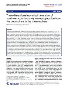
2 MATHEMATICAL MODEL OF THE TRAJECTORY 2.1 Motion Geometry The equations of motion that govern the trajectory Fig.1 of MSLV on the basis of structural mass fraction and centre of mass shift can be conveniently written in terms of its radial distance from the Centre of the earth r and velocity V . In addition, the position vector r is defined by its magnitude r , its longitude  L measured from the x -axis in the equatorial plane, positively eastward and its latitude L measured from the equatorial plane, along a meridian and positively northward,  is the flight path angle and  L is the azimuth or heading angle measured between positively in the right handed direction about the x -axis which define the velocity vector during the vehicle motions. These variables form the state vecT tor X  r , L , L ,V ,  ,  of the launch vehicle (in spherical and rotating earth coordinates). The Launch vehicles are propelled and controlled by thrust T and its corresponding deflection angle  , small deflections of the thrust vector control (TVC) engines  with respect to their nominal trim positions in pitch  p and yaw  y axis and for the first stage of the flight, controlled by deflections of the control surfaces  cs .Therefore inputs to the dynamic model are: Thrust T , control surface and engine deflections. These variables form the input force and moment vector T u  T ,  ,  of the launch vehicle. The effects of perturbations on the vehicle trajectories due to unmodeled vehicle dynamics, Earthary atmospheric rotation and composition, atmospheric forces and moments and wind gusts velocity are also considered. The aerodynamic forces act through the Centre of pressure, the force of gravity acts through the Centre of gravity, and the thrust force is applied through the "Centre of combustion. The Euler angles roll, pitch and yaw (  ,  , ) define the vehicle attitude [10] with respect to the inertial reference axes. In a launch vehicle the attitude reference is usually measured with respect to the launch pad with the Euler angles initially at (00,,900,00) respectively.The vehicle model outputs detectable by sensors are: attitude, attitude rates, rotation angle, angle of attack α and sideslip angle  . The assumption of a spherical rotating earth, atmosphere variation of density, pressure and gravity is eminently considered in the study. The reference axes are shown in Fig.1. with the x axis is aligned along the fuselage reference line and its direction is positive along the velocity vector. The z axis is defined posi-

IJSER 








467


tive downward towards the floor, and the y axis is defined by the right hand rule, perpendicular to the x and z axes and positive towards the right. The equations derived in this studies will consist of three rotational (roll, pitch and yaw), and three translational equations along x, y and z axes. The vehicle forces and moments generated in this model are calculated with respect to the body axes system.

x

Re V cos  Re  h

(3a)

h  V sin 

L 

(3b)

V cos  r cos L

(3c)

V cos  r T m Lsp g

L 

(3d) (3e)

m0  m f  m pr t 0 



(3f)



m  m t , X cg  m f  m pr t 





m t , X cg  m f  m pr (1 

T t) 1sp m0

(3g) (3h)

(0  t  t b )    t    

(3i) (3j) (3k)

V t  t b 

(3l)

V t b 

IJSER

Fig. 1. MSLV Flight Mechanics in Spherical Coordinate trajectory

2.2 The Equations of Translational Motion of the MSLV In this study, we model suitable representative equations of motion and corresponding optimum trajectory suitable for determination of a desired equilibrium of MSLV. Subsequently, the equation is linearized, and stability, controllability, and observability are analyzed. Through nonlinear simulation, we illustrate the extent to which linearized equations approximate the nonlinear ones. Creating flexible, software-defined test platform to validate deployed real-time embedded systems for control, monitoring, and operation. Trajectory waypoint and guidance law derivation in this study used a point-mass Launch vehicle model of the following form: V

T cos  T 1  cos   D   g sin   , h, L    mt  mt  mt 

 r cos L sin  cos L  cos  sin L 

(1)

2



T sin   L    V  mt V r

 2r V



g  cos   2V cos  L  V

cos  L cos  cos  L  sin  sin  L   Fd

(2)

The instantaneous altitude, longitude and latitude of the vehicle position fig.1 are obtained from the translational equations and defined equations 3a-3d.

The respective initial conditions depend on the launch time t L and on the launch site (identified by the geographical longitude, ls , and by the latitude,  ls ) ref[1]. These equations are then solved separately for each stage. In the above equations, r denotes the distance of the centre of gravity of the vehicle to the centre of the Earth, v is the modulus of its relative velocity,  is the flight angle (or path inclination, that is, the angle of the velocity vector with respect to an horizontal plane),  L is the latitude, L is the longitude, and  is the azimuth (angle between the projection of the velocity vector onto the local horizontal plane measured with respect to the axis South-North of the Earth). The aerodynamic forces consist of the drag force D , whose 2 modulus is 0.5 (h) SCDV , which is opposite to the velocity vector, and of the lift force, whose modulus is 0.5 (h)SCLV 2 which is perpendicular to the velocity vector.S is some positive coefficient (reference area) featuring the engine, CD and CL and are the drag and the lift coefficients; they depend on the angle of attack and on the Mach number of the vehicle. The drag coefficient CD depends on the shape of the rocket and the smoothness of its surface. The drag coefficient is one of the major unknown quantities that are usually determined through wind tunnel or flight test and will be simulated using the correlation of Aerodynamic Drag coefficient relations.

2.3 Aerodynamic Forces Aerodynamic forces are the result of the impact of the environment on the surface of the launch vehicle when it moves. They are defined as the sum of the elementary tangential and normal forces acting on the body of the launch vehicle. Depending on whether the moving body is symmetrical relative to the axis, or its axis of symmetry is directed in the motion


468


along the velocity vector or deviates from it, there appears one axial force (drag), side force and normal force (lift). The symbol D , S , L and donate respectively the drag, side force and normal force depending on the aerodynamics in clean configuration such as:

1  h SCDV 2 2 1 S   h SCV 2 2 1 L   h SCLV 2 2 Where C D is the drag coefficients, D

(4a)

g  g0

(4d)

(4e) Aerodynamics coefficient C D and CL can be represented in terms of angle of attack  ,Mach number M and Reynolds number Re . The drag coefficient C D depends on the shape of the rocket and the smoothness of its surface. The drag coefficient is one of the major unknown quantities that are usually determined through wind tunnel or flight test and will be simulated using the correlation of Aerodynamic Drag coefficient relations[] in this study as: For M  1.3 For M  1.3 CDMAX  0.067atM  1.3



C

D

h

h

 h  0.034e 6705.6

(5b)

The forces and torque generated are given by Launch vehicle is generated on account of combustion of fuel with mass flow rate and discharge of combustion products through the nozzles. The thrust

T model at a certain altitude h with nozzle exit

P

pressure a and pressure at a given height pressed as [1]:

T h  

mp tb

v e  Pa  Ph  n Ae

V P  , a  1.4  ah 

h  9144m

can be ex-

(6a)

Tvacmax 

mp tb

ve  Pa Ae

(6b)

Considering the parameters and the accuracy  n of the nozzle exit area, the expression for Tvac (h) at any height h in vacuum shall be modeled as:

Tvac h  Ts s   Tvacmax  PhAe 

(6c)

Where Ts (h) is the axial thrust from each stage of the MSLV and emphasize that the thrust is a function of time and height. Specific models of the gravity, the air density, air pressure and the aerodynamic coefficients are implemented for trajectory analysis solution in this study.

3 Optimum trajectory Flight formulation for MSLV

h  9144m

ph  101325 1  2.25577 10 5 h 

Ph

Where  n is the uncertainty in the precision of nozzle exit area Ae of the propulsion system of the stage. The interplay among the stated variables determines the thrust profile at sea level. In perfect vacuum (100%), Ph  0 and thrust reaches its maximum and can be expressed as

IJSER

 0.765 / M

1 2,M

(4f) And for the air density  , it decreases with altitude and the influence of drag is greatest at the lower altitudes. For analytical reasons it is convenient to use an exponential approximation to the atmosphere. One such approximation below 9144.0m altitude is given by[11]

 h  1.23366e 9144

RE  h 2

2.5 Thrust due to Main Engine and Small thrusters (4c)

CD  CD  , M , Re  CL  CL  , M , Re 

CD  0.25  1  M

RE2

(4b)

CY the side force coefficient CL the lift coefficient, S is the reference surface area for the rocket and  the air density [ref 18]. The coefficient C D and CL are function of angle of attack  ,Mach number M and Reynolds number Re .

2

Where L is the latitude and g 0 is expressed in meters per second squared. The formula is based on an ellipsoidal model of the earth and also accounts for the effect of the rotation of the earth. The variation of g with altitude g (h) is easily determined from the gravitational law as

(4g) 5.25588

T  T0  tg h 2.4 Gravity-Weight Accurate values of the gravitational acceleration as measured relative to the surface of the earth account for the fact that the earth is a rotating oblate spheroid with flattening at the poles is considered. These values may be calculated to a high degree of accuracy from the 1980 International Gravity Formula, which is

g 0  9.7803271  0.005279 sin 2  L  0.000023 sin 4  L

The determination of the optimal trajectories leading to insertion of satellites into desired mission orbit is an essential premise to the definition of the guidance strategy, and defines the best performance attainable by an MSLV with specified propulsive characteristics, such as that considered in this study. The considered state variables are velocity, thrust profile, altitude, and mass, whereas the control variable is the programmed angle of attack. The trajectory analysis computes the state variables by solving the equation of motion presented in Eq. 34, and evaluating the constraint conditions at every phase of flight

(5a) IJSER © 2015 http://www.ijser.org

469


Fig. 2. MSLV flight trajectory.

Significant variable cross section of MSLV imposed a new approach to trajectory design and optimization for its real applications. In this study, a first principle approach of modeling the trajectory flight of MSLV with stochastic parameters is presented in (1),(2).This guidiance command was generated on the basis of the set of differential equations, which describes its translational motion as a non-uniform body.

Adapting the MSLV as research object, and according to improved MSLV vehicle dynamic models, the waypoints of launch vehicle motion was established and generated in Matlab/Simulink on the basis of additional trajectory flight path model equations stated above. The non linear differential equations and the boundary conditions required are specified by the respective Simulink codes and results can be plotted for easy analytical predictions. From this derived model, several plots were made which describes the characteristics of the various parameters as encapsulated in the general equation governing the trajectory variables. The essential parameters considered as solution to the waypoint planning include the vehicle stages mass, model of the atmosphere, propulsion system, vehicle mass fraction geometric variation, coefficient of drag as a function of march numbers, gravity variation as a function of latitude and altitude, earth rotation effect and stages separations non-linearity. Adapting the MSLV as research object, and according to improved MSLV vehicle dynamic models, the waypoints of launch vehicle motion and the Launch Vehicle steering command was established and generated in Matlab/Simulink. The differential equations and the boundary conditions required are specified by the respective Simulink codes and results can be plotted for analysis. The nominal trajectory for a given mission is pre-computed and stored on-board. The nominal pitch rate is continuously updated by the guidance system such that it always equals the rate of change of flight path angle. The variation of the flight path angle during insertion flight has substantial influence on the injection accuracy in orbit, acceleration loads, and final orbital velocity. It is influenced by a programmed angle of attack.

IJSER

4 Model of Flight Path Angle

A novel tool for trajectory data generation scheme for turning flight and vertical phase on the basis of variable vehicle cross sectional areas is developed from quadratic curve of basic equation of trajectory motion He Linshu (2007).     0 i  0 i  0 i 2 2 2  t   2 2      22i  0 i , t 2 t 2 2i 1i   2  1i   2i  1i   2i 2

5 Initial Conditions

(7)

Where  (  ) is the flight path angle as a function of instantaneous vehicle mass fraction  , 1i is the mass fraction at time of turning the rocket trajectory from initial value and  2i is the mass fraction at the end of turning to desired final flight path angle  0 . i is the flight profile of stages.

Fig. 3. MSLV trajectory profile and Dynamics.

For a typical solid propellant LV orbital payload insertion, the trajectory starts from the launch site with initial altitude at sea level, the initial velocity of the launch site as a contribution to velocity gain and, the initial condition is also that the flight path angle should be ϑ 0=90 degrees, and the initial the angle of attack also should be zero degrees. In the equation of motion, the steering angle of the thrust,  is the only control variable to point and direct the rocket into desired direction. The lifting of rocket vertically corresponds to a steering angle of 90 degree and as the rocket achieves higher altitude, it begins to perform pitch over so that  is less than 90 degree, eventually, the rocket is travelling with  near zero. The performance index to this optimization is steering law,  (t ) , which is now modified as a function of time and variable cross sectional area so as to minimize its elastic behaviour The new function is a key component of algorithms for GNC system because it essentially equivalent to determining the trajectories and controls that transfer MSLV from Launch site to mission orbit. The mass and propulsive thrust is partition in the numerical solutions as follows:


470


 t f  tb,1 m0,1  m p ,1t f  m m0,3  m p ,3 t f  tb ,1  t f  tb ,1  tb , 2  m0,3  m p ,3 t f  tb , 2  tb ,1  t f  tb ,1  tb, 2  tb,3 T1 t f  tb ,1  T  T2  tb,1  tb , 2 T t  t  t  t f b ,1 b,2 b ,3  3

6.2 Stage waypoint variables for trajectory profile of MSLV.

(8)

6 Application of Numerical Simulation of Nonlinear models to MSLV Trajectory Usually launch vehicles translational motions are described by linear models that typically involve solving a set of simultaneous,(14) nonlinear partial differential equations by numerical methods. In principle, the numerical solution to trajectory optimization of Launch vehicles is based on point mass model of translational motion where the study of nonlinear events by such means is by and large intractable. Although there have been many analytical studies of one or another nonlinear effects, the system context is usually idealized or much simplified compared to realistic launch vehicle trajectory scenarios. In addition, it is typical for such analytical formulations to be of such complexity as to require numerical evaluation, a situation which negates the values of analysis—insight and generality. Perhaps the justification for the simulation approach to the solutions of launch vehicles waypoint planning in this study is the presence of nonlinear models of equation of motions and properties of the flight environment. A novel Simulink based numerical simulation approach for determining variable parameters and non-linear effects of the models of MSLV trajectory waypoints.is used to provide calculated time series trajectory of MSLV.This approach is assumed necessary for emerging MSLV flight control sensors, stages interface and payload due to their extremely small dimension and lower inertia masses.

Fig. 5. Simulink Blocks of Trajectory Simulator for 1st Stage

IJSER Fig. 6. Simulink Blocks of Trajectory Simulator for 2nd Stage

6.1 The Nonlinear simulation scheme of MSLV

Fig. 4. Simulink Blocks of Trajectory Simulator for Flexible MSLV

Fig. 7. Simulink Blocks of Trajectory Simulator for 3rd Stage


471


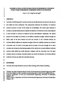
6.3 Simulink Simulation results of the flight trajectory The results obtained are presented in the curves shown below in Fig. 8-15. MSLV FLIGHT PATH ANGLE AGAINST TIME 100

ALTITUDE(Km) AGAINST RANGE(Km)

FLIGHT PATH ANGLE (Degree)

250

ALTITUDE(Km)

200

150 FLEXIBLE BODY BASED ON POINT MASS 100

50

0 -100

90 80

60 50 40 30 20 10 0

0

100

200

300

400

500

600

700

800

FLEXIBLE BODY NOMINAL

70

900

0

50

100

150

Fig.8. Altitude Vs Range

250

300

350

Fig. 10. Flight Path Angle Vs Time

IJSER

MSLV SPEED AGAINST TIME

MSLV ALTITUDE AGAINST TIME

9000

250


8000

200

7000

SPEED (Km/s)

ALTITUDE (Km)

200

TIME (Sec)

RANGE(Km)

150

100


50

6000 5000 4000 3000 2000 1000

0

0

50

100

150

200

250

300

0

350

0

50

TIME (Sec)

100

150

200

TIME (Sec)

Fig.9. Altitude Vs Time Fig.11. Speed Vs Time


250

300

350

472


DRAG(N) AGAINST ALTITUDE(Km)

MSLV THRUST AGAINST TIME

5

x 10

9

500 NOMINAL FLEXIBLE BODY

450

8

400


350

6

DRAG(N)

THRUST(KN)

7

5 4

300 250 200 150

3

100

2

50

1 0

0

0

50

100

150

200

250

300

0

50

100

150

200

250

H(Km)

350

TIME (Sec) Fig.15. Altitude Vs Drag

Fig.12. Thrust Vs Time

MSLV RANGE AGAINST TIME 900 FLEXIBLE BODY NOMINAL

IJSER

800 700

RANGE

600 500 400 300 200 100 0 -100

0

50

100

150

200

250

300

350

TIME (Sec)

Fig.16. Flight-path angle in gravity-turn trajectory (A.Tewari, 2011)

Fig.13. Range (Km) Vs Time

ALTITUDE AGAINST GRAVITY 250

200

H(Km)

150

100

50 Fig.14: Altitude Vs Gravity GRAVITY MODEL 0

9

9.1

9.2

9.3

9.4

9.5

9.6

9.7

9.8

9.9

10

GRAVITY(m/s 2)

Fig.17. Speed in gravity-turn trajectory (A.Tewari, 2011) Fig.14. Altitude Vs Gravity IJSER © 2015 http://www.ijser.org

473


control loops for a significant vehicle elastic displacenment.This tool demonstrated the importance of including flexibility and variable point mass structure into the coupled effect of slender body during trajectory motion. For the general case, the guidance system must maintain the vehicle on the nominal trajectories. This study can be applied for path planning for tailored trajectories for microsatellite deployment as well as missile defense type applications.

REFERENCES [1] Adetoro et al, (2014) Parameterization of Micro Satellite Launch Vehicle. Journal of Aeronautics & Aerospace Engineering, Volume 3 .Issue 2. 1000134 Fig.18. Radius in gravity-turn trajectory for launch from the Earth’s surface (A.Tewari, 2011).

6.4 Observation and Discussion of Results (Fig.8-18) In this study, we have presented simulation solution of nonlinear trajectory motions and environment of MSLV with the single greatest justification for the approach to launch vehicles waypoint planning in the presence of nonlinear elements. We have also demonstrated the realistic waypoint planning of the proposed solution by simulating the behaviour of this vehicle via variable mass fraction solution approach by application of Matlab/Simulink to Rungi Kutta numerical solutions and flight environment nonlinearities. The results compare favourably with existing analytical trajectory optimization techniques but also reveal the anticipated practical behaviours as obtained in actual vehicle flight. This solution can serve as a basis for control engineers to correct the trajectory due to model errors and unmodeled disturbances for integration into guidance and navigation tasks.The result of this solution scheme also reveals extra large transverse displacement and need for bending modes control due to sudden change of flight path angle during stages separation. The plots (Fig.8-15) validated the output of this tool because of its compatibility with realistic behaviour of VEGA Launch Vehicle Ref: Vega User’s Manual(2014)Source: www.arianespace.com.The profile of our result also agrees with results in literature as shown in fig. 4.21 page 224 (A.Tewari, 2011) and reveals trajectory errors of fig.4.27.page 226 (A.Tewari, 2011) as shown in fig.16.

[2] Adetoro L. and Aro H., “Nigeria Space Program”, Aerospace Guidance Navigation and Flight Control Systems (AGNFCS’09) Workshop, Samara, Russia. [3] Adetoro L., “Embedded System Control: Design and Implementation on Multifunctional Sounding Rocket Ground Testing Equipment”, Aerospace Guidance Navigation and Flight Control Systems (AGNFCS’09) Workshop, Samara, Russia.

IJSER

[4] Adetoro L., “Effective Method of Trajectory Control for Geostationary Communication Satellite”, proceeding of the Scientific Conference of SUAI devoted to the World Day of Aviation and Astronautics, April 12, 2010, Saint Petersburg, Russia. [5] Adetoro L., “Comparative Design of Attitude Stabilization and Control Schemes for three axes Space Vehicle”, Master Thesis on the Direction of Instrumentations, St Petersburg State University of Aerospace Instrumentation, September 22, 2010, Saint Petersburg, Russia.

[6] Adetoro L., “Space Vehicle Trajectory Control”, proceeding of the Scientific Conference of SUAI devoted to the World Day of Aviation and Astronautics, April 12, 2009, Saint Petersburg, Russia. [7] Adetoro L., Post Launch Campaign of Nigeria Communication Satellite (NigComSat-1), 2007.

7 Conclusion In this study we developed improved Simulink based path planning algorithm for three stage Launch Vehicle on the basis of nonlinear translational equations, physics of the atmosphere, solution approach of He Lisshu, 2007[] and non-rigid body using parameterization results of Adetoro et al,2014[].In results, we generate a nominal trajectories tools of a flexible flying vehicle for various trajectory problems as a solution to two-point boundary value problems. The result of the nonlinear trajectory simulation tool revealed the concealed discontinuity in flight path, at separation and anticipated damages to

[8] Agboola, O., Fashade.,K and Adetoro, L., “Optimization of Ascent Trajectory and Mass budget Prediction: A case Study for Center for Space Transport and Propulsion, Epe, Lagos State, Nigeria”, proceeding of the Scientific Conference of SUAI devoted to the World Day of Aviation and Astronautics, April 12, 2010, Saint Petersburg, Russia. [9] Agrawal, B. N. (1986), Design of Geosynchronous Space-


474


craft. Englewpod Cliffs, NJ: Prentice-Hall. [10] Fashade K., and Adetoro L., “Transfer Orbit Trajectory Controller Design for a Typical Spacecraft Launching from Nigeria”, IFAC conference 2010, Saint Petersburg, Russia. [11] Kaplan, M. H. (1976), Modern Spacecraft Dynamics and Control. New York: Wiley. [12] Lebsock, K. L. (1980), "High Pointing Accuracy with a Momentum Bias Attitude Control System," Journal of Guidance and Control 3(3): 195-202. [13] MATLAB® and Simulink® System, 2009. Mathworks, USA. [14] Sergey A. B., Adetoro L., and Aro H., “Intelligent Approach to Experimental Estimation of Flexible Aerospace Vehicle Parameters’’, Proceeding of ICON2009, Istanbul, Turkey. [15] Sidi, M.J., 1997. Spacecraft Dynamics and Control, Cambridge University Press, UK.

launch vehicle design” Journal of Spacecraft and Rockets, Vol. 34, No.4, pp 478-485, July-August,1997. [24] Tsuchiya, T. and Mori. T. “Multidisciplinary Design Optimization to future space transportation vehicle”. AIAA 20025171. [25] Szedula, J.A., FASTPASS: “A Tool for Launch Vehicle Synthesis”, AIAA-96-4051-CP, 1996. FASTPASS (Flexible analysis for synthesis trajectory and performance for advanced space systems) developed by Lockheed Martin Astronautics. [26] Anderson, m., Burkhalter J., and Jenkins R “Multidisciplinary Intelligence Systems Approach To Solid Rocket Motor Design, Part I: Single and Dual Goal Optimization”. AIAA 2001-3599, July, 2001. [27] M Balesdent, N Bérend, P Dépincé, “New MDO Approaches for Launch Vehicle Design”, 4th European Conference for Aerospace Sciences, St. Petersburg, Russia, (07/2011)

IJSER

[16] Singh,S.K.,and Agrawal,B.N., “Comparison of Different Attitude Control Schemes for Communication Satellites’’, American Institute of Aeronautics and Astronautics Conference, 1987.

[17] Surauer, M., Fichter, W., and Zentgraf, P., “Method for Controlling the Attitude of a Three-axis Stabilized, Earth Oriented Bias Momentum Spacecraft”, United States Patent number 5,996,941. Dec.7, 1999. [18] Thomson, W. T. (1986), Introduction to Space Dynamics. New York: Dover. [19] Wertz, J. R. (1978), Spacecraft Attitude Determination and Control. Dordrecht: Reidel.

[28] Božić.O, T. Eggers and S. Wiggen, “Aerothermal and flight mechanic considerations by development of small launchers for low orbit payloads started from Lorentz rail accelerator’’, Progress in Propulsion Physics 2 (2011) 765-784.

[29] Schneider, M.,Božić, O. and Eggers, T., "Some Aspects Concerning the Design of Multistage Earth Orbit Launchers Using Electromagnetic Acceleration," Plasma Science, IEEE Transactions on, vol.39, no.2, pp.794,801, Feb. 2011. [30] Teofilatto P and E. De Pasquale, “A fast guidance algorithm for an autonomous navigation system”, Planetary and Space Science, Volume 46, Issue 11, Pages 1627-1632(1998)

[21] Wie, B., 1998. Space Vehicle Dynamics and Control, AIAA Education Series.

[31] Michael Benjamin Rose, “Statistical Methods For Launch Vehicle Guidance, Navigation, And Control System Design And Analysis”, A Dissertation Submitted In Partial Fulfillment Of The Requirements For The Degree Of Doctor Of Philosophy in Mechanical Engineering, Utah State University Logan, Utah(2012)

[22] Stanley, D.O., Talay, A.T., Lepsch, R.A., Morris, W.D., Kathy, E.W. “Conceptual Design of a Fully Reusable Manned Launch System”. Journal of Spacecraft and Rockets, Vol 29, No.4, pp 529-537, July-August, 1992

[32] Dukeman, G., “Atmospheric Ascent Guidance for RocketPowered Launch Vehicles”, AIAA Paper 2002-4559, Proceedings of the AIAA Guidance, Navigation, and Control Conference, Monterey, CA, August 5-8, 2002.

[23] Braun, R.D. and Moore., “Collaborative approach to

[33] Alexander S. Filatyev, Alexander A. Golikov, “New

[20] Wertz, J.R., 1995. Spacecraft Attitude Determination and Control, Kluwer Academic Publisher, 73.


475


Possibilities Of Significant Improvement Of Aerospace Launcher Efficiency By Rigorous Optimization Of Atmospheric Flight”, 24th International Congress of the Aeronautical Sciences (2004). [34] Chaudenson J, D. Beauvois, S. Bennani, M. GanetSchoeller, G. Sandou, “Dynamics modeling and comparative robust stability analysis of a space launcher with constrained inputs”.2003 [35] Scott Schoneman, Mark Chadwick, and Lou Amorosi, “A New Space Launch Vehicle: Low Cost Access to Space Using Surplus Peacekeeper ICBM Motors”, A program managed by the Air Force Rocket Systems Launch Program (RSLP), SMC Det 12/RP (2003) [36] Roberto Rodrıguez, “Study of a nozzle vector control for a low cost mini-launcher”, Universitat Politecnica de Catalunya ,Master in Aerospace Science & Technology (2011)

IJSER
