Accepted for publication in: Applied Ocean Research 2007
Numerical simulation of fully nonlinear regular and focused wave diffraction around a vertical cylinder using domain decomposition W. Bai, R. Eatock Taylor* Department of Engineering Science, University of Oxford, Parks Road, Oxford OX1 3PJ, UK
Abstract The fully nonlinear regular and focused wave propagation and diffraction around a vertical circular cylinder in a numerical wave tank are investigated. The Mixed Eulerian-Lagrangian approach is used to update the moving boundary surfaces in a Lagrangian scheme, in which a higher-order boundary element method is applied to solve the wave field based on an Eulerian description at each time step. In order to increase the efficiency of the calculation, the domain decomposition technique is implemented, with continuity conditions enforced on the interface between adjacent subdomains by an iterative procedure. In this domain decomposition method, the top layers of elements at the interfaces are semi-discontinuous to avoid problems from the singularity. In addition, mesh regridding using the Laplace smoothing technique and interpolation are applied on the free surface to deal with possible numerical instability. Numerical results are obtained for the propagation of nonlinear regular waves and focused wave groups, and for the diffraction of such waves by a vertical cylinder. These results indicate that the present method employing the domain decomposition technique is very efficient, and can provide accurate results when compared with experiment data. Keywords: Fully nonlinear; Wave diffraction; Focused wave; Domain decomposition; Semi-discontinuous element
1. Introduction In recent years, as the offshore industry has moved towards deeper water and harsher environments, the problem of modelling the interactions of steep waves with offshore structures has become an increasing concern. For many years, first- and more recently second-order analyses in the frequency domain have been used to investigate the wave diffraction around a fixed structure. Examples of second-order analysis are given in Molin [1], Eatock Taylor and Hung [2], Kim and Yue [3], and Wu and Eatock Taylor [4]. Isaacson and Cheung [5], and Kim et al. [6] also developed a second-order time-domain method for the wave diffraction problem. However, these studies are still restricted in applicability, because water waves are fully nonlinear and unsteady. Based on the pioneering work of Longuet-Higgins and Cokelet [7] using the Mixed Eulerian- Lagrangian * Corresponding author. Tel.: +44 1865 273144; fax: +44 1865 273010. E-mail address:
[email protected] (R. Eatock Taylor).
1
(MEL) time stepping technique, fully nonlinear numerical wave tank models have been developed during the last two decades. Recent applications of this fully nonlinear approach to simulate nonlinear wave diffraction around bottom-mounted structures include Ma et al. [8], Turnbull et al. [9], and Wu and Hu [10], who developed numerical wave tanks based on the finite element model. The alternative boundary element method was used by Contento [11], and Koo and Kim [12], for simulations in a two-dimensional wave tank and by Ferrant [13] for three-dimensional simulations of the diffraction problem. Grilli et al. [14] and Xue et al. [15] have used the higher-order boundary element method to investigate three-dimensional overturning waves. It is known, however, that solving the mixed boundary value problem for φ directly for N boundary element nodes requires O(N2) operations, which is prohibitive when N exceeds several thousand. Even if, as here, the higher-order boundary element method is used, the computation of the three dimensional nonlinear simulation is still very demanding. As a result, previous investigations have often been restricted to small domains and short simulation times. Various attempts have been made to increase the computational efficiency, such as the Fast Multipole Method (e.g. Rokhlin [16], Fochesato and Dias [17]) and the domain decomposition method. Here, domain decomposition is investigated and applied. This method has already been adopted in other research fields, for example in structural dynamics (Farhat and Li [18]), aeroacoustics (Arina and Falossi [19]) and modelling explosions (Dean and Glowinski [20]). In computational hydrodynamics, the domain decomposition method has received less attention: only Wang et al. [21] and De Haas and Zandbergen [22] appeared to have used this approach in a two dimensional implementation. It is particularly suitable for the parallel computing, as implemented for example by Cai et al. [23] and Guo et al. [24]. The basic idea of domain decomposition is to divide the computational region into many subdomains, and to apply the boundary element method to each individual subdomain, leading to far fewer unknowns in each subdomain compared with in the original region. Thus, the computational effort per subdomain is much reduced. The key issue in domain decomposition is to satisfy suitable continuity requirements between adjacent subdomains. This can lead to two alternative approaches. One is to define unknowns on both sides of the common surfaces between adjacent subdomains. Only one block-diagonalised coefficient matrix then needs to be assembled with contributions from all the subdomains (Wang et al. [21]). Another approach is to match the values of variables on the common surfaces through a suitable iteration procedure, with the assembly and solution of the coefficient matrix carried out in each independent subdomain (De Haas and Zandbergen [22]). By contrast to the coefficient matrix in a volume-discretised approach, such as the finite element method, the submatrices arising from the first domain decomposition approach described above are full and unsymmetric, which makes the problem expensive to solve even though it is block-diagonalized. The second approach is more convenient to implement using parallel computing, because each processor can almost finish the computation in the corresponding subdomain independently of the information from other subdomains. We therefore use here the domain decomposition based on the iteration procedure, which generates a sequence of boundary conditions on the interfaces between the subdomains.
2
This paper is based on an extension of the numerical method presented by Bai and Eatock Taylor [25]. They gave details of a higher order boundary element for fully nonlinear wave problems, and applied it to analysis of radiated waves excited by a forced oscillating cylinder undergoing surge, heave, pitch, and combinations of these motions. The aim of the present paper is to apply the domain decomposition method in the development of a numerical wave tank. The increase in computational efficiency thereby achieved is directed towards facilitating practical design. Numerical results are obtained for regular wave propagation, as well as for wave diffraction around a fixed vertical circular cylinder in a three-dimensional wave tank. In the design of offshore structures for realistic seas, behaviour in extreme waves must be modelled. The largest waves represent an individual event within a random sea state, and may be simulated by focusing wave components such that individual wave crests simultaneously come into phase at one point in space. The NewWave theory is based on this focused wave idea (Tromans et al. [26]). In this paper, such focused waves are investigated numerically, and compared with the results of physical experiments (Baldock et al. [27]). Moreover, some particular features of nonlinear focused wave diffraction are also studied, to clarify the change in the position of the focus point with respect to the cylinder which results from nonlinear effects. We are not aware of such simulated results for focused wave diffraction having been previously published.
2. Higher-order boundary element simulation To simulate numerically the wave diffraction in a three-dimensional wave tank, a right-handed Cartesian coordinate system Oxyz having the origin O on the mean water surface and z-axis pointing vertically upwards is defined as shown in Fig. 1. The fluid is assumed to be incompressible and inviscid, and the motion irrotational. The water wave problem can be formulated in terms of a velocity potential φ(x, y, z, t), which satisfies Laplace’s equation within the fluid domain Ω, and is also subject to various boundary conditions on all instantaneous surfaces S of the fluid domain. Once the potential has been found by solving the mixed boundary value problem at each time step, the pressure on the body is expressible using the Bernoulli equation. The wave forces F = {f1, f2, f3} and moments M = {f4, f5, f6} can consequently be obtained by integrating the pressure over the wetted body surface. Here, some auxiliary functions ψi (i = 1,…,6) are introduced, in place of computing φt in the Bernoulli equation directly (details can be found in Wu and Eatock Taylor [28]). These functions satisfy Laplace’s equation in the fluid domain, and the corresponding conditions on the boundary surfaces. Finally, the wave force is given by the following expression f i = −ρ
∫∫
SB +SF
∫∫ [
]
1 ⎛ ⎞ ∂ψ i ds − ρ ψ iU& 0 − ∇ψ iU 0 (∇φ − U 0 i ) ds , ⎜ gz + ∇φ ⋅ ∇φ ⎟ 2 ⎝ ⎠ ∂n S
(1)
M
where ρ is the density of the fluid, g is the acceleration due to gravity, n is the normal unit vector pointing out of the fluid domain, U0 is the velocity of the piston-like wave maker moving only in the x direction assumed here, and U0i term means that it has the value of U0 only in the x direction. This second mixed boundary value problem for ψi has the same type of conditions (Neumann or Dirichlet) on the same
3
boundary surface as the mixed boundary value problem for φ, which means these two different problems share the same influence coefficient matrix. z Beach
y x
O
SF
SB
n
SM
SW
SD
Fig. 1. The sketch of definition
In this paper, the higher-order boundary element method is used to solve the mixed boundary value problem at each time step. In this numerical method, the surface over which the integral is performed is discretised by quadratic isoparametric elements. After introducing shape functions Nj(ξ, η) in each surface element, one can write the position coordinate, the velocity potential and its derivatives within an element in terms of nodal values, in the following forms: x(ξ , η ) =
K
∑
φ (ξ , η ) =
N j (ξ , η )x j ;
j =1
∂φ (ξ , η ) = ∂ξ
K
∑
K
∑N
j
(ξ ,η )φ j ;
(2a)
j =1
∂N j (ξ , η )
j =1
∂ξ
φj ;
∂φ (ξ , η ) = ∂η
K
∑ j =1
∂N j (ξ , η ) ∂η
φj ,
(2b)
where K is the number of nodes in the element, xj and φj are the nodal positions and potentials, and (ξ, η) are local intrinsic coordinates. By substituting these representations into the boundary integral equation, the resulting discretised equation can be finally expressed in the matrix form (Bai and Eatock Taylor [25]): ⎡ A (11) ⎢ ( 21) ⎢⎣ A
A (12) ⎤ ⎧⎪ X (1) ⎫⎪ ⎧⎪ B (1) ⎫⎪ ⎥⎨ ⎬=⎨ ⎬, A ( 22) ⎥⎦ ⎪⎩X ( 2) ⎪⎭ ⎪⎩B ( 2) ⎪⎭
(3)
where
{
}
X (1) = φ1 , φ 2 , L , φ N n ; Ai(,11j ) = C (x i ) + Ai(,21j ) ; Ai(,12j ) = Ai(,22j ) = −
Np
⎧⎪⎛ ∂φ ⎞ ⎛ ∂φ ⎞ ⎛ ∂φ ⎞ ⎫⎪ X ( 2) = ⎨⎜ ⎟ , ⎜ ⎟ , L , ⎜ ⎟ ⎬ ; ⎝ ∂n ⎠ N p ⎪⎭ ⎪⎩⎝ ∂n ⎠1 ⎝ ∂n ⎠ 2 Ai(,21j ) =
Nn
∑∑ [G(x
M
⎡ ∂G (x m , x i ) ⎤ N j (ξ , η )wm J m (ξ , η ) ⎥ ; ∂n ⎦ n =1 m =1
∑∑ ⎢⎣
M
m , xi )N j
(3a)
(ξ ,η )wm J m (ξ ,η ) ] ;
n =1 m =1
4
(3b) (3c)
Bi(1) =
Nn
M
⎡
∑∑ ⎢⎣G(x
m , xi )
n =1 m =1
∂φ (x m ) ⎤ wm J m (ξ , η ) ⎥ − ∂n ⎦
(3d) ⎡ ∂G (x m , x i ) ⎤ ( 2) (1) φ (x m )wm J m (ξ , η ) ⎥ ; Bi = −C (x i )φ (x i ) + Bi . ⎢ ∂n ⎦ n =1 m =1 ⎣ Here, Nn and Np are the numbers of elements on the Neumann and Dirichlet boundaries respectively, M is Np
M
∑∑
the number of sampling points used in the standard Gauss-Legendre method to evaluate numerically the integration over each element, wm is the integral weight at the mth sampling point, Jm(ξ, η) is the Jacobian transformation from the global to the local intrinsic coordinates. We notice that the solid angle C(xi) at the field point xi still needs to be determined. Here, a convenient formula expresses it as an integration of the derivative of the Green’s function (Wu and Eatock Taylor [29]), which can be obtained directly from the influence coefficients without additional work.
3. Domain decomposition For the purposes of illustration, the computational domain Ω with prescribed boundary conditions is decomposed into the subdomains Ω1 and Ω2 which are separated by an interface Γ. On the interface, the potential and its normal derivative are not known a priori, and an initial guess of Dirichlet condition φ(0) or Neumann condition ∂φ(0)⁄∂n needs to be imposed. If φ equals the exact solution of the Laplace’s equation in the original domain on the interface location, then the normal derivatives of the potential ∂φ1⁄∂n1 and ∂φ2⁄∂n2 in domains 1 and 2 will be continuous because of the uniqueness of the Laplace’s equation. In the same way, the exact solution of ∂φ⁄∂n on the interface will lead to a continuous potential over the interface. Therefore, the stop criterion on the interface for convergence of the iterative solution can be written as ⎧ ⎪ φ1 (x) − φ 2 (x) < ε φ ⎪ , ⎨ ⎪ ∂φ1 (x) + ∂φ 2 (x) < ε n ⎪ ∂n1 ∂n 2 ⎩
(4)
where εφ and εn are the tolerances corresponding to φ and ∂φ⁄∂n, and n1 and n2 point out of domains 1 and 2 respectively. There are different ways to construct the iteration sequence finding the exact value of φ and ∂φ⁄∂n on the interface and the procedure used here is the following scheme, referred to as the D/D-N/N scheme (De Haas and Zandbergen [22]): 0. Choose an initial Dirichlet condition φ (k), (k=0). 1. Solve the Laplace’s equation in Ω1 and Ω2 with the Dirichlet condition φ1(k)= φ2(k)= φ (k) on Γ. This yields ∂φ1(k)⁄∂n1 and ∂φ2(k)⁄∂n2 on Γ. 2. Formulate a Neumann condition ∂φ(k+1)⁄∂n by taking an average of the computed solutions,
5
(k ) ∂φ ( k ) ∂φ ( k +1) 1 ⎛⎜ ∂φ1 = − 2 ∂n ∂n 2 2 ⎜⎝ ∂n1
⎞ ⎟. ⎟ ⎠
(5)
3. Solve Laplace’s equation with the Neumann condition
∂φ1 ( k +1) ∂φ ( k +1) ∂φ ( k +1) =− 2 = ∂n1 ∂n 2 ∂n
on Γ. This
yields φ1(k+1) and φ2(k+1) on Γ. 4. Formulate a Dirichlet condition φ (k+2) by taking an average of the computed solutions,
5.
(
)
1 ( k +1) φ1 + φ 2 ( k +1) . 2 Calculate the maximum error ε(k+2) on Γ, based on the potential obtained in Ω1 and Ω2,
φ ( k + 2) =
ε ( k + 2) = max φ1 ( k +1) − φ 2 ( k +1) .
(6)
(7)
6. If ε(k+2) satisfies the prescribed stop criterion, then exit the loop, and the final approximate solutions on the interface are φ (k+2) and ∂φ(k+1)⁄∂n. 7. Go to step 1 and repeat the procedure with k=k+2. In the case of more subdomains the scheme can be extended straightforwardly by performing each step in the scheme on all subdomains and for all interfaces simultaneously. In the numerical approach the Laplace equations are solved with the boundary element method in all subdomains separately. Anticipating the resources required by the boundary element method, the following implications with respect to storage and efficiency can be given: •
By introducing the interfaces, extra boundary elements and nodes are needed. However, because the memory required per subdomain depends quadratically on the number of nodes in the considered subdomain, the total required memory can be reduced considerably, depending on the number of interfaces.
•
A similar comment may be made in relation to the computation time required to assemble the coefficient matrix, which only needs to be determined at the beginning of the iterative procedure, since the geometry does not change during the iteration.
•
There is a similar reduction of the required computation time for solving the linear algebraic system at each iteration step.
At the same time, it is important to note that we only generate a sequence of boundary conditions on the interfaces and that the conditions on the outer boundaries are fixed during the iteration process.
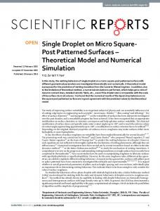
4. Singularity on interfaces In the D/D-N/N scheme discussed above, we need to solve Laplace’s equation in each subdomain with the Dirichlet and Neumann conditions on the interfaces at alternate iterative steps. On the free surface another Dirichlet condition is specified. Therefore, a problem appears on the intersection line between the free surface and the interface, where some double nodes are distributed. Because these double nodes share the same position and the same type of boundary condition, their coefficients obtained by Eq. (3c) will be
6
exactly the same: this will result in a singular algebraic equation system. To deal with this difficulty, semi-discontinuous elements are used here. Before explaining the semi-discontinuous element approach, we review the functions of the nodes within each boundary element. They can serve three purposes. Firstly, they define the shape of the boundary element. Secondly, they are used to specify the unknowns within each boundary element. Thirdly, they are used as collocation points. We can consequently consider three separate sets of nodes named according to their function as geometric nodes, functional nodes and collocation nodes respectively. In the present semi-discontinuous element approach, the geometric nodes and functional nodes are coincident but are staggered from the collocation nodes in order to avoid singular matrices. The collocation nodes are placed inside elements, while the geometric nodes and functional nodes are still located on the edges of elements. As a result Eq. (3c) will yield different coefficients due to the different positions of the collocation nodes xi. To specify the positions of the new collocation nodes, we define a discontinuity coefficient γ in the frame of the local intrinsic coordinates, as shown in Fig. 2. The range of this coefficient is from 0 to 1, and the discontinuous element would become continuous if γ=1. From the figure, we also note that the semi-discontinuous element approach is only adopted in elements located at the interfaces and adjacent to the free surface, and on the free surface the normal continuous elements are used. Moreover, the staggered collocation nodes only replace the three double nodes on one side of each quadrilateral semi-discontinuous element; this is the reason why the elements here are called “semi-discontinuous”. A similar semi-discontinuous boundary element method has also been used by Subia et al. [30] and Guzina et al. [31] for different problems. In their approaches, the functional and collocation nodes were coincident but were staggered from the geometric nodes. It can be noted that in our method the collocation nodes are located at different places from the functional nodes, as mentioned above; this avoids using different shape functions within the semi-discontinuous elements. Once the positions of the new collocation nodes xi are known, the coefficients in Eqs. (3b), (3c) and (3d) can be determined. The known value φ(xi) in Eq. (3d) also needs to be changed: it should be taken as the value on the new position of the collocation point, obtained by use of the shape functions. Another modification is the calculation of the singular integration, where the triangular polar-coordinate transformation (Eatock Taylor and Chau [32]) should be performed on the new sub-triangles defined by the new collocation points.
7
η Continuous element on free surface
Double nodes
New collocation points
γ ξ
0
Semi-discontinuous element on solid surface Fig. 2. The definition of the semi-discontinuous element
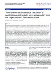
5. Numerical implementation In the application of the numerical method to simulate nonlinear water waves, a number of aspects related to the detailed performance have to be considered, which have a direct bearing on success or failure of the calculation. The details of the methods used can be found in Bai and Eatock Taylor [25]. Only some necessary illustrations and supplements are discussed here. In the present method, structured quadrilateral meshes are adopted on the vertical solid surfaces, and unstructured triangular meshes are generated on the free surface by using the Delaunay triangulation method. A double or triple node is employed on the intersections between the free surface and vertical surfaces. Fig. 3 shows meshes generated by this method for a fixed vertical circular cylinder in a wave tank, in which three subdomains are involved. Z Y
X
Fig. 3. An example mesh generated in a wave tank for illustration of the mesh generation
In order to avoid numerical instability, mesh regeneration on the free surface is used, leading to the need
8
to specify the horizontal coordinates of the new nodes. Interpolation is then used to predict the vertical coordinate, and the potential at the new node. It should be noted that in the domain decomposition approach, this horizontal mesh regridding should not be applied just within each subdomain independently, as this would result in a bad distribution of elements over the interfaces (no information being transferred in that case between adjacent subdomains). We need to treat the free surface as a whole, and apply the Laplacian smoothing technique on the whole free surface. The solution of the full and asymmetric influence matrix arising from the mixed boundary value problem at each time step is a significant part of the calculation. In general, the semi-discontinuous element approach provides slightly better conditioned matrix equations, but the convergence is still very slow when using an iterative scheme, such as the GMRES procedure. Therefore, the LU decomposition method is used here. As the number of unknowns is small in each subdomain, the computational effort is not very large using this method. Because the coefficient matrix only depends on the geometry that is unchanged in the iterative process, there are only two types of coefficient matrix, corresponding to the problems with Neumann and Dirichlet boundary conditions respectively. We can compute the matrix factorisations once, which can be used on all odd and even steps of the iterative process, and then use the back substitution afterwards.
6. Numerical results 6.1 Overview In this section we investigate the application of the domain decomposition method to four cases of propagating waves in a numerical tank. The first concerns regular waves in the absence of a diffracting body, and the second case extends the wave propagation model to consider the focusing of a nonlinear wave at a prescribed focus position and time. The parameters chosen are the same as in physical experiments by
Baldock et al. [27]. The third and fourth cases investigate the diffraction of these two types of wave, regular and focused, by a vertical cylinder in the numerical tank. The regular wave diffraction results are compared with experimental data given by Huseby and Grue [33], and other numerical results obtained by Ferrant [13]. 6.2 Regular wave propagating in a wave tank In the presentation of these results, we take the water depth d, gravitational acceleration g and fluid density ρ to be unity. Parameters such as distances are effectively non-dimensionalised. The wave maker is situated at x=-7.7, and the total tank length is 15.7. Only half of the wave tank is considered in this and the following sections due to symmetry, and the half-width is taken as 0.31. At the left end of the wave tank, a monochromatic wave is generated by a piston-like wave maker undergoing the following motion:
9
⎧S 0 (t ) = − a cos(ω t ) , ⎨ ⎩U 0 (t ) = aω sin(ω t )
(8)
where S0(t) and U0(t) are the displacement and velocity of the wave maker respectively, and a and ω are the motion amplitude and frequency of the wave maker. Near the right hand end of the wave tank, the damping zone is situated, based on the method described in Bai and Eatock Taylor [25]: this starts at a distance of one incident wavelength measured from the far end of the tank. In this case, the whole computational domain is divided into 10 subdomains of equal size. We first examine the convergence of the computation with the control parameters. We compute the propagating wave generated by the wave maker moving at a=0.01 and ω=2.0 with three different meshes, chosen as shown in Table 1. For each wave period, 20 time steps are chosen to perform the calculation for each of these meshes, in order to compare the CPU times. There are 6 elements in the vertical direction on the solid surfaces for all the cases in this paper. Figure 4 shows the wave profiles at two time instants, for prescribed values of γ and ε,
and the corresponding time history of the wave elevation at x=-3.12 is shown
in Fig. 5. The results converge very fast with the mesh size, and the results obtained with all three meshes are very close. Very careful examination of Fig. 5 reveals some apparent very slight discontinuities in the time history of elevation calculated at a specified position, x=-3.12. This is because the elevation actually plotted is that calculated at the nearest node to x=-3.12 at a given time step. We have also tested the stop criterion ε in Eq. (7) by changing its value from 1×10⁻⁴ to 1×10⁻⁵ with mesh b. The results indicate that ε=1×10⁻⁴ gives converged calculations, and this value is used in all the cases below. The discontinuous coefficient γ has also been investigated using two different values, 0.2 and 0.6, and all the results have been compared with those obtained without domain decomposition, with the same mesh density throughout. We find that the results seem to be independent of the discontinuous coefficient. A larger value of the coefficient, γ=0.9, has also been tried, but the computation aborts due to the very badly conditioned coefficient matrix arising from the mixed boundary value problem. A discontinuous coefficient of 0.6 has therefore been used in all the calculations. It has been found that with these parameters the results obtained with the domain decomposition method agree very well with those using a single domain, which suggests that the domain decomposition approach presented here is accurate. Table 1. Numbers of elements and nodes for different meshes in each subdomain
Mesh a Mesh b Mesh c
Intervals on the boundary of free surface (x×y)
Elements on free surface
Total elements
Total nodes
10×2 15×3 20×4
42 94 166
1260 2200 3340
4280 6840 9800
10
3
-4
mesh a, 10 , 0.6 -4 mesh b, 10 , 0.6 -4 mesh c, 10 , 0.6 single domain
2
z/a
1 0 -1 -2 -3
-5
-4
-3 x
-2
-1
(a) 3
mesh a, 10-4, 0.6 -4 mesh b, 10 , 0.6 -4 mesh c, 10 , 0.6 single domain
2
z/a
1 0 -1 -2 -3
-5
-4
-3 x
-2
-1
(b) Fig. 4. Convergence of the wave profile with different meshes at a=0.01: (a) t=7.5T; (b) t=15T -4
3
mesh a, 10 , 0.6 -4 mesh b, 10 , 0.6 -4 mesh c, 10 , 0.6 single domain
2
z/a
1 0 -1 -2 -3
0
3
6
t/T
9
12
15
Fig. 5. Convergence of the wave elevation at x=-3.12 with different meshes at a=0.01
Next, the efficiency of the domain decomposition method is investigated for the same case of a=0.01 and ω=2.0. With the domain decomposition, the computations use meshes a, b and c respectively. In the single domain, corresponding meshes with equal numbers of elements on the free surface and side walls are adopted. Because of the existence of the interfaces, the total numbers of nodes and elements in the whole domain are different for the cases with and without domain decomposition. Fig. 6(a) shows the comparison of CPU time for these three different meshes, normalised by the time for the finest mesh when domain decomposition is not used. It can be seen that without domain decomposition, the CPU time increases rapidly with increase in number of elements. Roughly 80% of the time is associated with solving the linear algebraic equations. On the other hand, the CPU time reduces to a nearly linear dependence on number of elements using domain decomposition. When the number of elements on the free surface is smaller than 500, the CPU time for these two methods is comparable, but domain decomposition is much more efficient if many elements are involved in the domain. We have also compared the normalised CPU time for cases with different numbers of subdomains, as shown in Fig. 6(b). We see that when the number of subdomains
11
exceeds a certain value (around 20 in this figure), the computer time increases. The reason is that when too many subdomains are used, the iteration times become larger due to the transfer of information between more interfaces; this results in more CPU time even though each subdomain has fewer elements. However, domain decomposition will save computer time whatever the number of subdomains is, and in all cases presented in the following around 10 subdomains are used. with domain decomposition without domain decomposition
1.2
0.3
1
CPU
0.2
CPU
0.8 0.6 0.4
0.1
0.2 0
0
500
1000
1500
0
2000
elements on free surface
0
5
10
15
number of subdomains
(a)
20
25
(b)
Fig. 6. Comparison of the computer time at a=0.01: (a) with and without domain decomposition for different meshes; (b) for different numbers of sub-domains
The efficiency of the artificial damping layer in absorbing reflected waves (Bai and Eatock Taylor [25]) has also been investigated here. . The comparison of the wave profiles at two time instants with that obtained in a longer wave tank (total length increased to 23.55), with a=0.01 and ω=2.0, is shown in Fig. 7. We can see that all the results are in good agreement, which indicates that there are no obvious waves reflected from the far end of the computational domain. It also can be seen how the propagating wave decays in the damping zone. The corresponding time history of the wave elevation at x=-3.12 is shown in Fig. 8. This figure confirms that the artificial damping layer works well. The same remarks apply about continuity in the time history, as discussed above. 3 short wave tank long wave tank
2
z/a
1 0 -1 -2 -3
-4
0
4 x
(a)
12
8
12
16
short wave tank long wave tank
3 2
z/a
1 0 -1 -2 -3
-4
0
4 x
8
12
16
(b) Fig. 7. Comparison of the wave profile in tanks of different length with a=0.01: (a) t=25T; (b) t=30T short wave tank long wave tank
3 2
z/a
1 0 -1 -2 -3
0
3
6
9
12
15 t/T
18
21
24
27
30
Fig. 8. Comparison of the wave elevation at x=-3.12 in tanks of different length at a=0.01
Figure 9 gives the spatial profiles of propagating waves at the incident wave frequency ω = 2.0, for three different amplitudes of the wave-maker motion: a=0.01, 0.02 and 0.043 respectively. These correspond to the resulting waves having steepnesses ε=H/λ ≈ 0.025, 0.05 and 0.085, where H is the wave height and λ the wave length. It should be noted that for the smaller incident amplitude case, a=0.01, the computation is stable without mesh regeneration, due to the weak non-linearity of the propagating wave. With the increase of amplitude corresponding to a=0.02 and 0.043, saw-tooth instability occurs. Remeshing is therefore applied every time step, which avoids overly distorted meshes. It can be seen from Fig. 9(a) that at t=7T the steady state wave has not yet reached the damping zone, whereas in Fig. 9(b) at t=15T it has occupied the whole wave tank. We can observe the expected non-linear behaviour, namely that the waves generated with the larger amplitude of the wave-maker motion have flatter troughs and sharper crests, also having longer wavelengths, and the wave profile and its amplitude are asymmetric about the mean position z=0. The corresponding time history of the wave elevation at x=-3.12 is shown in Fig. 10. It can be seen that the wave with larger amplitude travels faster than that with smaller amplitude. Again Fig. 10 shows evidence of small discontinuities for the same reason as discussed above. 3 a=0.01 a=0.02 a=0.043
2
z/a
1 0 -1 -2 -3
-6
-4
-2
0
x
13
2
4
6
8
(a) 3
a=0.01 a=0.02 a=0.043
2
z/a
1 0 -1 -2 -3
-6
-4
-2
0 x
2
4
6
8
(b) Fig. 9. Wave profile with different motion amplitudes of the wave maker at ω =2.0: (a) t=7.5T; (b) t=15T 3 2
a=0.01 a=0.02 a=0.043
z/a
1 0 -1 -2 -3
0
3
6
t/T
9
12
15
Fig. 10. Wave elevation at x=-3.12 with different motion amplitudes of the wave maker at ω =2.0
6.3 Focused wave in the wave tank In this section, focused waves are investigated to verify the ability and accuracy of the present method. The numerical simulations reproduce the experiment made by Baldock et al. [27], in which highly nonlinear wave-wave interactions were described. The wave tank was 20 m long, 0.3m wide and had a maximum working depth of 0.7m. These authors assumed that the focus position is located at x=0, and the focus time is t=0. A linear wave solution then gives the required surface elevation generated at the wave maker as
η (xP , t) =
N
∑A
n
cos(k n x P − ω n t ) ,
(9)
n =1
where N is the total number of wave components, An, kn and ωn are the amplitude, wave number and wave frequency of the nth wave component respectively, and xP is the position of the wave maker according to the linear prediction. From this equation, we obtain the linear wave amplitude at the focus position as A=
∑
N n =1
An .
A piston-like paddle is used as the wave maker. The relationship between the input signal and the resulting surface elevation, which affects the generation of a desired wave group, can be defined by a first order transfer function T(a, ω), such that A(ω ) = T (a, ω )a (ω ) . (10) Here A(ω) is the amplitude of the surface profile measured at the focus position, and a(ω) represents the
amplitude of the sinusoidal input signal at a wave frequency ω. Baldock et al. [27] determined this transfer
14
function experimentally using an appropriate range of regular wave trains, in order to avoid the uncertainty associated with a theoretical prediction. In the present simulations, the transfer function is obtained numerically. By simulating regular waves with five different wave periods T in the range 0.6 to 1.4, we repeated this range of wave period for three different amplitudes of the input signal a, to establish the influence of the wave amplitude on the transfer function. The calculations were performed in a wave tank which is 10λ long, 0.2λ wide and with a depth of 0.7m. Fig. 11 shows the resulting transfer functions showing that the transfer function is insensitive to wave amplitudes in this range. This makes it possible to find a single curve-fit for the points in the figure, facilitating the generation of other desired waves by simple interpolation.
transfer functions
2.5
2
-4
a=7.6*10 a=1.3*10-3 -3 a=1.9*10 fitting curve
1.5
1
0.6
0.8
1
T
1.2
1.4
Fig. 11. Transfer functions for different motion amplitudes of the wave maker
We now simulate the focused waves identified as cases B and C in the experiment by Baldock et al. [27]. Case B is a wave group with a broad-band spectrum in which the wave periods range from 0.6 to 1.4s; while Case D is a wave group with a narrow-band spectrum in which the wave periods range from 0.8 to 1.2s. Each group consists of 29 individual wave components, which are of equal amplitude, and equally spaced within the appropriate period range. Because we are only interested in the wave surface near the focal point around the focal time, a smaller tank is adopted here compared with that in the experiment. The present wave tank is 10m long and 0.14m wide, and the distance from the wave maker to the expected focal point under the linear assumption is 5m. The typical wave frequency and wave length used in the damping zone are chosen as the mean value and the maximum value of all wave components respectively. 12 subdomains are applied, and remeshing is not needed. Figs. 12 and 13 show the time histories of the surface elevation at the focal point for Cases B and D with three different input wave amplitudes (A=22mm, 38mm, and 55mm). As the hypothetical focused wave is assumed to be the linear sum of the individual wave components, it omits the effect of nonlinear wave-wave interactions. As a result, both the focal point and the focal time in the simulation and in the physical experiment are initially unknown. In the experiment, the focus position was determined experimentally for each wave group. In our numerical calculations, the focal time and focal position were predicted as follows. Around the expected linear focus time, we output the surface profile at many time instants. By comparing these, the position of the maximum wave elevation can be found, which is regarded as the focus point, with
15
an associated focus time. However, the mesh on the free surface moves at every time step, which makes it difficult to specify the time history of the wave elevation exactly at this focal point. This relates to the point discussed above in connection with Fig. 5. Therefore, we also output the time history of the wave elevation at several nodes around the expected linear focal point, and obtain the final results using interpolation. It should be noted that in the figures shown below, both the focal position and the focal time are shifted to zero, in order to compare with linear predictions. From Figs. 12 and 13, we can see that with the smallest input amplitude, the numerical results for both Case B and Case D agree well with the linear solution, confirming that the nonlinearity is very weak in this case. As the input amplitude is increased, the numerical results diverge from the linear solution gradually. The wave crest at the focal position is larger and narrower, while the wave troughs are wider and less deep, due to the stronger nonlinear interactions between wave components. The present numerical results are also very close to those in the experiment (Fig. 5 and 6 in Baldock et al. [27]), except in Case D with the highest input amplitude. In Fig. 13(c), the wave trough in the numerical results is deeper than that in the experiment.
1.2
1.2 linear results A=0.022
0.8
z/A
0.4
z/A
0.4 0
0
-0.4
-0.4
-0.8
linear results A=0.038
0.8
-1
-0.5
0 t/s
0.5
-0.8
1
-1
-0.5
(a)
0 t/s
0.5
1
(b)
1.2 linear results A=0.055
0.8 z/A
0.4 0
-0.4 -0.8
-1
-0.5
0 t/s
0.5
1
(c) Fig. 12. Time history of the surface profile at the focal point for Case B: (a) A=0.022m; (b) A=0.038m; (c) A=0.055m
16
1.5
1.5 linear results A=0.022
1
linear results A=0.038
1
z/A
0.5
z/A
0.5 0
0
-0.5
-0.5
-1
-1
-0.5
0 t/s
0.5
-1
1
-1
-0.5
(a)
0 t/s
0.5
1
(b) 1.5 linear results A=0.055
1
z/A
0.5 0 -0.5 -1
-1
-0.5
0 t/s
0.5
1
(c) Fig. 13. Time history of the surface profile at the focal point for Case D: (a) A=0.022m; (b) A=0.038m; (c) A=0.055m
Fig. 14 showing the maximum crest elevations at the focal point for different input amplitudes confirms again that the focusing of wave components produces a highly nonlinear wave group in which the nonlinearity increases with the input wave amplitude and reduces with increasing bandwidth. Based on the results obtained for Case B and Case D, the shifts of focal position and focal time due to nonlinear effects are shown in Fig. 15. The downstream shift of the focus point can be seen clearly in Fig. (15a), becoming larger with the increase of the input wave amplitude. The occurrence of the focusing event is increasingly delayed as the nonlinearity of the wave group increases. We find from the comparison with the results in the experiment, that the present numerical estimates of the focal position and the focal time are somewhat under-predicted at the highest input wave amplitude, especially for Case D.
17
1.4
z/A
1.2 1 linear results Case B Case D
0.8 0.6 0.01
0.02
0.03
A/m
0.04
0.05
0.06
Fig. 14. Crest elevations for different amplitudes 1.6
0.8 Case B Case D Case B, experiment Case D, experiment
0.6 focal time/s
focal point/m
1.2
0.8
0.4
0.4
0 0.01
Case B Case D Case B, experiment Case D, experiment
0.2
0.02
0.03
A/m
0.04
0.05
0 0.01
0.06
(a)
0.02
0.03
A/m
0.04
0.05
0.06
(b) Fig. 15. (a) Position of the focal points; (b) Time of focusing
6.4 Regular wave diffraction around a vertical cylinder Next, the wave diffraction around a fixed vertical cylinder in a rectangular wave tank is calculated. The cylinder of radius r=0.1416 is situated at the origin of coordinates. The wave tank is similar to that used in the simulation of propagating waves discussed in the first section, except that the half-width of the tank is doubled to 0.62 in order to reduce the reflections of radiated waves by the tank side walls (we have not so far considered very wide tanks, because of computer resource limitations). The wave maker is placed at x=-7.0, and the total tank length is reduced to 11.3, which can decrease the computational effort. The mesh density is largely the same as that used for the investigation of regular wave propagation, with a finer mesh near the body surface: 16 elements are distributed around one half of the cylinder at any level. In addition, the whole domain is divided into 9 subdomains. Figure 16 gives the time history of the force acting on the cylinder in the x-direction, for the case of waves generated at frequency ω=2.0 with the amplitude of the wave-maker motion being set at a=0.01 and a=0.02 respectively. The corresponding results for wave run-up at the extreme up-wave and down-wave points at the intersection of the cylinder and the free surface are shown in Figure 17. It can be seen from these figures that the wave force oscillates synchronously with the wave run-up on the upstream side of the cylinder, and the phase shift between the wave forces at different wave-maker motion amplitudes reflects
18
again the fact that nonlinear waves propagate faster than linear waves. The effect of the nonlinearity plays a more important role in the wave run-up than that in the wave force, because the calculation of the wave force is an integral over the body surface, which can cancel out some nonlinear influences. It may also be
seen that the downstream runup is particularly sensitive to nonlinear effects, and there is evidence in Fig. 17(b) of a lack of periodicity (perhaps due to the reflections or accumulated numerical error). 15 a=0.01 a=0.02
10
2
Fx/r a
5 0 -5 -10 -15
15
16
17
t/T
18
19
20
Fig. 16. Wave forces for different motion amplitudes of the wave maker at ω=2.0 incident wave a=0.01 a=0.02
6 4
z/a
2 0 -2 -4
15
16
17
t/T
18
19
20
18
19
20
(a) incident wave a=0.01 a=0.02
6 4
z/a
2 0 -2 -4
15
16
17
t/T
(b) Fig. 17. Wave run-ups for different motion amplitudes of the wave maker at ω=2.0: (a) upstream side; (b) downstream side
Fig. 18 shows the wave profiles on the line of symmetry along the x-direction at different time steps with a=0.02. From this figure, we can see clearly the process of how the wave flows past the cylinder, and the maximum wave run-up occurring at the downstream side. The wave run-up profiles around the cylinder at different time steps are illustrated in Fig. 19 for the case with a=0.01 and a=0.02 respectively. The steeper wave profile in Fig. 19(b) shows more complex features than the smaller amplitude case in Fig. 19(a).
19
t=17.0T t=17.2T t=17.4T t=17.6T t=17.8T
5 4 3 z/a
2 1 0 -1 -2 -3 -1.5
-1
-0.5
0 x
0.5
1
1.5
Fig. 18. Wave elevations on the line y=0.0 at different time instants with a=0.02 and w=2.0 t=17.0T t=17.2T t=17.4T t=17.6T t=17.8T
4
3
2
2
1
1
z/a
z/a
3
0
0
-1
-1
-2
-2
-3
0
50
100 degree
t=17.0T t=17.2T t=17.4T t=17.6T t=17.8T
4
-3
150
(a)
0
50
100 degree
150
(b)
Fig. 19. Wave profiles on the waterline of the cylinder at different time instants with ω =2.0: (a) a=0.01; (b) a=0.02
In order to assess the accuracy of the present numerical method, the wave forces acting on a vertical circular cylinder are compared with experimental data (Huseby and Grue [33]) and other numerical results (Ferrant [13]) for several values of wave steepness kA. The analysis by Ferrant was for a cylinder in the open sea. The experiment was carried out in a wave tank, which is 24.6m long, 0.5 m wide and filled with water to a depth of 0.6m. In the interest of saving computer time, a wave tank of smaller horizontal size is used in our calculation. Two different cylinders were used in the experiments, and only one of them (r=0.03m) is chosen here. We have made the comparison for an incident wave having non-dimensional wave number kr=0.245, the case which was also considered by Ferrant [13]. As discussed by Huseby and Grue [33], the drag force due to viscous effects can be expected to be small under these conditions. The wave forces were analysed by taking the Fast Fourier Transform over 5 wave periods after the steady state had been reached, to evaluate the first seven harmonic components. The comparison of these first and higher-harmonic wave loads is shown in Fig. 20 (and we reiterate that for practical reasons it was impossible to avoid the numerical results and the experimental data all being subject to slightly different effects from tank side walls). From the comparison, it can be seen that all our numerical results are in quite good agreement with both the experimental data and the numerical results of Ferrant [13], even at the seventh-harmonic force component. In particular, the second- and fourth-harmonic forces appear to agree better with the experimental measurements than with the other numerical results. Our predicted third-harmonic force, however, is larger and the fifth-harmonic force is smaller than the experimental data. In addition, it should be noted that the higher-harmonic forces are extremely small when kA is small, making 20
it very difficult to extract, for example, the sixth- and seventh-harmonic forces for such small kA at low wave steepness. The same problem was observed by Huseby and Grue [33] in their analysis of the experimental data. 7.2
Experimental data (Huseby and Grue [31]) Numerical results (Ferrant [13]) Numerical results (present analysis)
6.8
F1/pgAr
2
+
+ +
6.4
6
0
+
+
0.05
+
++
+
0.1
kA
0.15
0.2
0.25
(a)
+ + + +
2
F2/pgA r
0.6
+
+
+
+
++
Experimental data (Huseby and Grue [31]) Numerical results (Ferrant [13]) Numerical results (present analysis)
0.4
0.2
0
0
0.05
0.1
kA
0.15
0.2
0.25
(b) 0.6
+ 0.4 F3/pgA
3
+ + + +
+
+
+
Experimental data (Huseby and Grue [31]) Numerical results (Ferrant [13]) Numerical results (present analysis)
++
0.2
0
0
0.05
0.1
kA
0.15
0.2
0.25
(c) 0.6
F4/pgA r
4 -1
+
Experimental data (Huseby and Grue [31]) Numerical results (Ferrant [13]) Numerical results (present analysis)
0.4
+ + +
+
+
0.2
0
0
0.05
0.1
+
++
kA
(d)
21
0.15
0.2
0.25
0.4
F5/pgA r
5 -2
0.3
+ +
+
0.2
+
Experimental data (Huseby and Grue [31]) Numerical results (Ferrant [13]) Numerical results (present analysis)
++
0.1 0 0.05
0.1
0.15 kA
0.2
0.25
(e) 0.3
+
F6/pgA r
6 -3
+ +
0.2
Experimental data (Huseby and Grue [31]) Numerical results (Ferrant [13]) Numerical results (present analysis)
++ 0.1
0 0.05
0.1
0.15 kA
0.2
0.25
(f)
F7/pgA r
7 -4
0.6
+
+ +
0.4
Experimental data (Huseby and Grue [31]) Numerical results (Ferrant [13]) Numerical results (present analysis)
++ 0.2
0 0.05
0.1
0.15 kA
0.2
0.25
(g) Fig. 20. Comparisons of wave forces on the cylinder with experimental data and other numerical results: (a) first-harmonic force; (b) second-harmonic force; (c) third-harmonic force; (d) fourth-harmonic force; (e) fifth-harmonic force; (f) sixth-harmonic force; (g) seventh-harmonic force
6.5 Focused wave diffraction by a vertical cylinder Finally, we investigate the diffraction of a focused wave by a bottom-mounted cylinder in the wave tank. In section 6.3, we have calculated the focused wave propagation problem, which is chosen as the incident wave here. Only one input wave condition is studied, which corresponds to Case B with A=0.055m (see Fig. 12c). The width of the wave tank is now doubled to 0.6m, and a cylinder of radius 0.2m is placed in the middle of tank. Three cases are computed, corresponding to the wave focusing at different positions relative to the cylinder. Fig. 21 shows the time histories of wave force on the cylinder for the three cases with the wave focusing at the centre of the cylinder, on the upstream side and on the downstream side respectively. It can be seen that the wave force is not symmetric around the focal time, unlike the incident focused wave close to the
22
focus. We also note that the maximum positive wave force occurs when the focal point is on the downstream side of the cylinder, while the maximum force in the opposite direction arises when the focal point is on the upstream side of the cylinder. middle upstream side downstream side
4
2
Fx/pgr A
2 0 -2 -4 -4
-3
-2
-1
0 t/s
1
2
3
4
Fig. 21. Time history of the wave force on the cylinder around the focal time for different focal positions
Fig. 22 shows the time histories of wave run-up on the upstream and downstream sides of the cylinder, corresponding to the same three focus positions, together with the incident wave. In Fig. 22(a), we observe that the wave run-up is synchronous with the wave force for these three cases. When the wave focuses on the upstream side of the cylinder, the wave run-up is largest, and the maximum occurs very close to the focal time. The wave run-up becomes smaller when the focal point moves to the downstream side of the cylinder. Moreover, with the focal point at the middle of the cylinder a symmetric wave run-up is produced around the focal time. For the wave run-up on the downstream side in Fig. 22(b), the maximum is almost the same as that of the incident focused wave, except for when the wave is focused on the upstream side. middle upstream side downstream side incident wave
3
1
2
z/A
z/A
2
1
0
0
-1
-1 -1
-0.5
0 t/s
0.5
middle upstream side downstream side incident wave
3
1
-1
(a)
-0.5
0 t/s
0.5
1
(b)
Fig. 22. Time history of the wave run-ups on the cylinder around the focal time for different focal positions: (a) upstream side; (b) downstream side
The wave profiles at different time instants along the line of symmetry in the x direction, and around the cylinder, are given in Figs. 23 and 24 respectively. From these figures, it can be seen that the waves near the downstream side of the cylinder are very similar for these three different cases of focus position, while they are quite different near the upstream side of the cylinder.
23
3
3 t=-0.28s t=-0.18s t=-0.08s t=0.02s t=0.12s
t=-0.18s t=-0.08s t=0.02s t=0.12s t=0.22s
2
z/A
z/A
2
1
0
1
0
-1 -1.5
-1
-0.5
0 x/m
0.5
1
-1 -1.5
1.5
-1
-0.5
(a)
0 x/m
0.5
1
1.5
(b) 3 t=-0.38s t=-0.28s t=-0.18s t=-0.08s t=0.02s
z/A
2
1
0
-1 -1.5
-1
-0.5
0 x/m
0.5
1
1.5
(c) Fig. 23. Wave elevations on the line y=0.0 at different time instants for the focal point at: (a) the middle of the cylinder; (b) the upstream side of the cylinder; (c) the downstream side of the cylinder t=-0.28s t=-0.18s t=-0.08s t=0.02s t=0.12s
3
2
z/A
z/A
2
1
0
-1
t=-0.18s t=-0.08s t=0.02s t=0.12s t=0.22s
3
1
0
0
50
100 degree
-1
150
(a)
0
50
100 degree
(b)
24
150
t=-0.38s t=-0.28s t=-0.18s t=-0.08s t=0.02s
3
z/A
2
1
0
-1
0
50
100 degree
150
(c) Fig. 24. Wave profiles on the waterline of the cylinder at different time instants for the focal point at: (a) the middle of the cylinder; (b) the upstream side of the cylinder; (c) the downstream side of the cylinder
7. Conclusions Fully nonlinear regular and focused waves propagating in a wave tank, as well as their diffraction around a fixed vertical circular cylinder, have been simulated by using a higher-order boundary element model with the domain decomposition technique. The numerical results for the regular wave propagation problem indicate that the domain decomposition technique used here is efficient, especially for large numbers of elements in the computational domain. Based on calculations for a wave tank of length 10λ and unit dimensionless depth, with different numbers of subdomains, we find that calculations with 10 to 20 subdomains in this case are most efficient. As the amplitude of the wave maker motion is increased, numerical instability can occur when the nonlinearity is strong. The diffraction problem is particularly susceptible to such instability, when sharp corners can occur between adjacent elements on the free surface adjacent to the cylinder, leading to singularities in the boundary element equations. The remeshing and interpolation methods presented here can help avoid this instability, without causing serious numerical diffusion; and refined meshes with reduced time steps may also be used. Focused waves were also generated, and comparison of the wave profiles with experimental data has shown that the present numerical method is accurate. We have also compared the wave force on a cylinder with experimental results and other published numerical results, under the condition of regular incident waves. The first- to seventh-harmonic wave force components were extracted and found to be in satisfactory agreement with the other results. We also simulated the focused wave diffraction problem. We found that the maximum wave force in the positive direction occurs when the focal point is on the downstream side of the cylinder, while the focal point being located on the upstream side of the cylinder results in the maximum force in the opposite direction. It is also found that the wave run-up on the upstream side of the cylinder is largest for the case with the focal point located on the upstream side of the cylinder.
Acknowledgements
25
The authors gratefully acknowledge the financial support provided by the Engineering and Physical Sciences Research Council (EPSRC) Grant GR/S56917, and use of Oxford Supercomputing Centre resources.
References [1] Molin B. Second-order diffraction loads upon three-dimensional bodies. Appl Ocean Res 1979; 1: 197-202. [2] Eatock Taylor R, Hung SM. Second-order diffraction forces on a vertical cylinder in regular waves. Appl Ocean Res 1987; 9(1): 19~30. [3] Kim MH, Yue DKP. The complete second-order diffraction solution for an axisymmetric body. Part 1. Monochromatic incident waves. J Fluid Mech 1989; 200: 235-264. [4] Wu GX, Eatock Taylor R. The second order diffraction force on a horizontal cylinder in finite water depth. Appl Ocean Res 1990; 12: 106-111. [5] Isaacson M, Cheung KF. Time-domain second-order wave diffraction in three dimensions. J Waterway, Port, Coastal & Ocean Eng, ASCE 1992; 118: 496~516. [6] Kim Y, Kring DC, Sclavounos PD. Linear and nonlinear interactions of surface waves with bodies by a threedimensional Rankine panel method. Appl Ocean Res 1997; 19: 235-249. [7] Longuet-Higgins MS, Cokelet CD. The deformation of steep surface waves on water: I. A numerical method of computation. Proc R Soc Lond A 1976; 350: 1-26. [8] Ma QW, Wu GX, Eatock Taylor R. Finite element simulation of fully non-linear interaction between vertical cylinders and steep waves - part 1: methodology and numerical procedure. Int J Numer Meth Fluids 2001; 36: 265-285. [9] Turnbull MS, Borthwick AGL, Eatock Taylor R. Numerical wave tank based on a σ–transformed finite element inviscid flow solver. Int J Numer Meth Fluids 2003; 42: 641-663. [10] Wu GX, Hu ZZ. Simulation of nonlinear interactions between waves and floating bodies through a finite-element-based numerical tank. Proc R Soc Lond A 2004; 460: 2797-2817. [11] Contento G. Numerical wave tank computations of nonlinear motions of two-dimensional arbitrarily shaped free floating bodies. Ocean Eng 2000; 27: 531-556. [12] Koo W, Kim MH. Freely floating-body simulation by a 2D fully nonlinear numerical wave tank. Ocean Eng 2004; 31: 2011-2046. [13] Ferrant P. Fully nonlinear interactions of long-crested wave packets with a three dimensional body. In: Proceedings of the 22nd ONR Symposium on Naval Hydrodynamics, Washington, U.S.A. 1998. p. 403-415. [14] Grilli ST, Guyenne P, Dias F. A fully non-linear model for three-dimensional overturning waves over an arbitrary bottom. Int J Numer Meth Fluids 2001; 35: 829-867. [15] Xue M, Xü H, Liu Y, Yue DKP. Computations of fully nonlinear three-dimensional wave-wave and wave-body interactions. Part 1. Dynamics of steep three-dimensional waves. J Fluid Mech 2001; 438: 11–39. [16] Rokhlin V. Rapid solution of integral equations of classical potential theory. J Comp Physics 1985; 60: 187-207. [17] Fochesato C, Dias F. A fast method for nonlinear three-dimensional free-surface waves. Proc R Soc Lond A 2006; 462: 2715–2735. [18] Farhat C, Li J. An iterative domain decomposition method for the solution of a class of indefinite problems in computational structural dynamics. Appl Numer Math 2005; 54: 150-166. [19] Arina R, Falossi M. Domain decomposition technique for aeroacoustic simulations. Appl Numer Math 2004; 49: 263-275. [20] Dean EJ, Glowinski R. Domain decomposition methods for mixed finite element approximations of wave problems. Computer and Math with Appl 1999; 38: 207-214.
26
[21] Wang P, Yao Y, Tulin MP. An efficient numerical tank for non-linear water waves, based on the multi-subdomain approach with BEM. Int J Numer Meth Fluids 1995; 20: 1315-1336. [22] De Hass PCA, Zandbergen PJ. The application of domain decomposition to time-domain computations of nonlinear water waves with a panel method. J Comp Physics 1996; 129: 332-344. [23] Cai X, Pedersen GK, Langtangen HP. A parallel multi-subdomain strategy for solving Boussinesq water wave equations. Advance in Water Resource 2005; 28:215-233. [24] Guo Y, Jin X, Ding J. Parallel numerical simulation with domain decomposition for seismic response analysis of shield tunnel. Advance in Eng Software 2006; 37: 450-456. [25] Bai W, Eatock Taylor R. Higher-order boundary element simulation of fully nonlinear wave radiation by oscillating vertical cylinders. Appl Ocean Res 2006; 28(4): 247-265. [26] Tromans PS, Anaturk AR, Hagemeijer P. A new model for the kinematics of large ocean waves-applications as a design wave. In: Proceedings of the 1st Int Offshore and Polar Eng Conf, Edinburgh, UK. 1991; 3: p. 64-71. [27] Baldock TE, Swan C, Taylor PH. A laboratory study of nonlinear surface waves on water. Phil. Trans. of the Royal Society of London Ser. A 1996; 354: 649-676. [28] Wu GX, Eatock Taylor R. The coupled finite element and boundary element analysis of nonlinear interactions between waves and bodies. Ocean Eng 2003; 30: 387-400. [29] Wu GX, Eatock Taylor R. The numerical solution of the motions of a ship advancing in waves. In: Proceedings of the 5th Proc Int Conf on Numerical Ship Hydrodynamics, Hiroshima, Japan. 1989. p. 386-394. [30] Subia SR, Ingber MS, Mitra AK. A comparison of the semidiscontinuous element and multiple node with auxiliary boundary collocation approaches for the boundary element method. Engineering Analysis with Boundary Elements 1995, 15: 19-27. [31] Guzina BB, Pak RYS, Martinez-Castro AE. Singular boundary elements for three-dimensional elasticity problems. Engineering Analysis with Boundary Elements 2006, 30: 623-639. [32] Eatock Taylor R, Chau FP. Wave diffraction theory – some developments in linear and non-linear theory. J Offshore Mech and Arctic Eng 1992; 114: 185-194. [33] Huseby M, Grue J. An experimental investigation of higher-harmonic wave forces on a vertical cylinder. J Fluid Mech 2000; 414: 75-103.
27