Reynolds stress model for aircraft design applications. o Investigation of the .... compared to the performance of a desktop computer more than 30 years later. This increase made it ..... builders/users have over their system. As the cluster scene ...
Linköping Studies in Science and Technology Thesis No. 1246
Application of Parallel Computers to Enhance the Flow Modelling Capability in Aircraft Design
MATTIAS SILLÉN
Division of Applied Thermodynamics and Fluid Mechanics Department of Mechanical Engineering Linköpings universitet SE-581 83 Linköping, Sweden Linköping 2006
Copyright © 2006 by Mattias Sillén Distributed by Department of Mechanical Engineering Linköpings universitet SE-581 83 Linköping, Sweden LiU-TEK-LIC-2006:27 ISBN 91-85523-82-8 ISSN 0280-7971 Printed by LiU-Tryck, Linköping 2006 II
Abstract The development process for new aircraft configurations needs to be more efficient in terms of performance, cost and time to market. The potential to influence these factors is highest in early design phases. Thus, high confidence must be established in the product earlier than today. To accomplish this, the concept of virtual product development needs to be established. This implies having a mathematical representation of the product and its associated properties and functions, often obtained through numerical simulations. Building confidence in the product early in the development process through simulations postpones expensive testing and verification to later development stages when the design is more mature. To use this in aerodynamic design will mean introducing more advanced physical modelling of the flow as well as significantly reducing the turn around time for flow solutions. This work describes the benefit of using parallel computers for flow simulations in the aircraft design process. Reduced turn around time for flow simulations is a prerequisite for non-linear flow modelling in early design stages and a condition for introducing high-end turbulence models and unsteady simulations in later stages of the aircraft design process. The outcome also demonstrates the importance of bridging the gap between the research community and industrial applications. The computer platforms are very important to reduce the turn around time for flow simulations. With the recent popularity of Linux–clusters it is now possible to design cost efficient systems for a specific application. Two flow solvers are investigated for parallel performance on various clusters. Hardware and software factors influencing the efficiency are analyzed and recommendations are made for cost efficiency and peak performance.
III
IV
List of papers This thesis is based on the following two papers: I.
M. Sillén, “Advanced Flow Simulation Methods in Aircraft Design”, Aircraft Engineering and Aerospace Technology, Vol. 74, No. 2, 2002, pp. 138–146.
II.
M. Sillén, “Evaluation of Parallel Performance of an Unstructured CFD Code on PC– Clusters”, Journal of Aerospace Computing, Information, and Communication, Vol. 2, February 2005, pp. 109–119.
V
VI
Contents Abstract
III
List of papers Contents
V VII
1 Introduction
1
2 Aims
3
3 The role of CFD in aircraft design
5
3.1
Design environment
5
3.2
Background
7
4 Numerical method
11
4.1
Basic solver technique
11
4.2
Flow modelling
12
4.3
Computational models
14
4.4
Parallelization
16
4.5
Load balancing
17
4.6
Examples of current aircraft applications
17
5 Parallel computer platforms
19
5.1
Parallel architecture
19
5.2
Evaluated systems
21
6 Performance measurements
23
VII
7 Summary of papers
27
8 Conclusions
29
9 Outlook
31
10 Acknowledgments
33
11 Bibliography
35
Paper I Paper II
VIII
1 Introduction Computational Fluid Dynamics (CFD) is the science of generating numerical solutions to a system of partial differential equations which describe fluid flow. CFD is done with discrete methods and the purpose is to better understand qualitative and quantitative physical phenomena in the flow which then is often used to improve upon engineering design. CFD brings together a number of different traditional disciplines: fluid dynamics, the mathematical theory of partial differential systems, computational geometry, numerical analysis and computer science. The current challenges in the aerospace field are to offer products that are both better in performance and also faster and cheaper to produce. Thus the current business market forces aircraft designers towards risk minimization and a definitive reduction in cost and time to market [1]. The possibility to influence life cycle cost is largest in the early design stages. This means that the confidence in the design must increase in the early phases compared to today. Introducing high fidelity simulations early in the design process will facilitate this if the turn around time requirement can be met. In early phases the allowable time frame to conduct flow simulations is very limited, in extreme cases in the order of minutes. Also in later design stages there is a need to reduce the total simulation wall time to allow for more advanced physical modelling or increased resolution that due to computational cost not are feasible today. A recent example from Airbus with the development of the A380 wing illustrates the challenges. The wing design required the computer simulations of over 800 design proposals for which the computer analyses were carried out over a period of two years. To reduce this to 3 months, as the market may demand for a future aircraft of even more complexity, will require at least an order of magnitude increase in design efficiency and productivity. A significant reduction in turn around time of a design can be accomplished by carrying out the design activities simultaneously in each discipline using simulation and optimization tools. This work is usually carried out in groups working in close cooperation. To accomplish this, a mathematical model of the product is needed. This concept of using a high fidelity mathematical/numerical representation of the physical properties and the functions of the product is often called a virtual product (VP). Critical to the success of the VP is the capability for rapid generation of high fidelity information from all disciplines, which recent advances in information technologies and high performance computer systems now have enabled. Figure 1 presents a vision of what the VP offers to aircraft design. Using the VP generates more and better knowledge about the design during the earlier design phases
1
Chapter 1 resulting in an improved final design because the fidelity of the design is higher and available earlier in the process. This will eventually reduce the number of design cycles, the development risks, the number of flight tests, the cost and time to market.
⇒ The vision: 1 representation fidelity
verification in flight tests
higher fidelity earlier verification in ground facilities
VP
0
product definition
flight testing: - improvement and verification of data, e.g. aerodynamic data set
classical
ground-facility testing: - design improvement - design verification - data-set generation product development
time
Figure 1 Illustration of the benefit of the virtual product in aircraft design, namely higher fidelity in the design earlier in the cycle. The development of the Dassault FALCON F7X business jet [2] presents a similar picture as the A380 wing development. The use of the VP concept in the development process has increased compared with previous designs and computer simulations and optimizations are routinely used. However, the aerodynamic design still represents a significant part of the time to market and a significant reduction is expected to the next generation business jet. For the FALCON F7X aerodynamic design more than 500 3D (three-dimensional) full aircraft Navier–Stokes calculations were performed. Key factors in the analysis process were rapid unstructured mesh generation and efficient flow solvers on parallel computers that allowed for data generation of a complete polar in a matter of days. To further reduce the development time improvements are needed both in the physical modelling capability and flow solver turn around time. The necessity of high fidelity modelling in the design process is often conflicting with the requirement of short turn around time. A balance between modelling requirement and turn around time limitation needs to be established at every phase in the design cycle. A way to reduce the turn around time is to use powerful parallel computer systems. Traditionally, supercomputer resources have been equivalent with large cost and therefore not widespread in industry. This started to change in the late 1990s when PC–cluster with Linux, so called Beowulf systems, became popular. Larger and application specific computer systems are now designed using cheap commodity components. When designing a PC–cluster for a specific application several design choices have to be made. The selection of computer node configuration and interconnecting network are major factors influencing the parallel performance. Making the better choices will provide improved performance of the flow solver and thereby offering a chance to improve the modelling capability or reducing the turn around time.
2
2 Aims The aim of this study is to increase the confidence in the aerodynamic design by extending the flow modelling capability in the design process. This is done following two paths: o Improving the confidence in the simulations by introducing an explicit algebraic Reynolds stress model for aircraft design applications. o Investigation of the factors influencing the flow solver efficiency on parallel computers. Methods and tools must reach a level of maturity before they are allowed to enter the aircraft design process. This means that the leading edge of modelling technology in the design process will differ from what it the leading edge in the research community. Technologies being developed at universities and research establishments will often require some years of refinement and tuning before they are validated and acknowledged to enter the design process. This study covers a period when much of the aerospace industry introduced a new generation of flow solvers based on unstructured grids. This shift in methodology is mainly governed by the turn around time requirements for the complete CFD solution process, not only the raw performance of computers and flow solvers. This is an important industrial aspect of modelling capability – the ability to deliver reliable results in a limited time frame.
3
4
3 The role of CFD in aircraft design 3.1 DESIGN ENVIRONMENT The design of aircraft is an extremely interdisciplinary activity involving numerous engineering disciplines. The design task is to achieve an optimal integration of all components into an efficient, robust and reliable aircraft with high performance that can be manufactured with low technical and economical risk at an affordable cost over the whole lifetime of the aircraft. The aircraft design process is in general divided into three phases which tend to overlap in a staggered fashion. This is elaborated in more details in [3] with focus on aerodynamic design. In the conceptual design phase the aircraft is defined at a system level. Many variants are studied, and the design selected is the one that bests fulfils the specifications of the market or a customer. In the preliminary design phase the tentatively selected concept is refined until feasibility is established, i.e. extensive array of design sensitivities are generated, design margins, etc. About two–thirds of the way through this phase, the concept is frozen and no major changes are expected thereafter unless serious problems arise. The final phase is the detailed design phase in which details of the product are elaborated, optimizations are made and data sets are generated. A large variety of aerodynamic tools are used in each phase of the design process, including empirical/handbook methods, wind tunnel testing, flight testing and numerical simulation and optimization tools. In general, low fidelity tools are supposed to be used in the conceptual design phase where many alternatives are to be analyzed in a short period, while high fidelity tools are used in the other design phases since the concept evolves to an acceptable level of maturity. The term fidelity refers to the representation of the aircraft geometry and of the physical modelling. To locate the role of CFD in the design process and the relationship to the computing platform different levels of functionality of the integrated design process is described in Figure 2.
5
Chapter 3 Integrated Design Environment
Flight mechanics
Weight/balance
Structural design
Flight control Product Definition Management Engine aircraft performance
Aero-elasticity
Aerodynamics
Aerodynamic environment Handbook methods
CFD methods
WT-tests
CFD environment Geometry modeller
Grid generation
Solver
Visualization
Navier-Stokes solver Physical modelling Computer implementation
Computing platform
Numerical modelling software
hardware
Figure 2 Functionality of four layers of integrated interdisciplinary aircraft design. At the highest level, the integrated design environment, the disciplines of aerodynamics, structures, flight mechanics and flight control etc. all interact through a product data management system (PDM) to determine the configuration and characteristics of the aircraft. The second layer focuses on aerodynamics where CFD simulations are playing an increasingly important role in design. The CFD solution process in the third layer covers the geometry modelling, the grid generation, flow solver and data visualization. On the level of the flow solver the designer selects the physical model for the CFD simulation according to the design stage, ranging from conceptual to detailed design. A suitable balance must be found between solution accuracy and turn around time. This covers both the physical modelling as well as the mesh resolution. The turn around time is also influenced by the solver efficiency which depends strongly on the relationship between the computer implementation and the computing platform.
6
The role of CFD in aircraft design Within the integrated design environment the different disciplines run their design processes concurrently with interfaces to each other via the common PDM system. This is described in the flow chart in Figure 3. The process covers all the design phases and a number of iterations are performed to improve and optimize the design. In the conceptual design phase much of the analysis is performed with handbook methods or panel methods while nonlinear methods (Euler and Navier–Stokes) are usually employed in later stages. Szodruch [4] presents a similar example of the aerodynamic wing design that illustrates the process used at Airbus.
CFD Solver
Linear
Concept-Definition: Size, Requirements, Range, Mission, Performance Interface Basic Wing Params: Airfoil section, Planform, AR, Λ, λ, Mcr, etc. Disciplines
Non-linear Analysis & Optimization
Structures
Aerodynamik design
Control
iterations
Design check
Dynamics iterations
Model Manufacturing Wind tunnel tests Results Analysis Complex, Refined Analysis High Credibility
Systems etc.
Design Check
1st Wing Definition Performance Database
Figure 3 Integrated and concurrent aerodynamic wing design. Returning to the vision for the virtual product development process – The virtual product vision is to have very high representation fidelity already in the product definition phase. This presents a huge challenge for computational simulations. High fidelity simulations must be performed earlier than today and more advanced physical methods must enter the design process. To accomplish this the turn around time must be significantly reduced and state of the art flow modelling methods must reach industrial maturity for integration in the aerodynamic design process.
3.2 BACKGROUND The use of CFD in aircraft design started in the 1960s. Initially it was used to supplement wind tunnel testing and flight testing, but has now matured to a technology of its own, contributing to all stages of the design process. This development is mainly governed by three factors:
7
Chapter 3 o Significantly increase of available computer resources. o Development of efficient numerical algorithms. o Enhancements in physical modelling. Several authors have reviewed aspects of these developments extensively; see for recent examples [5, 6, 7]. Here only a brief summary is given to set the stage of the current use of CFD in aircraft design. In the 1960s and early 1970s CFD in aircraft design consisted of simplified (linear) models, i.e. the Laplace or the Prandtl–Glauert equations solved mainly by panel methods. Panel methods are still widely used in early stages in the design cycle. The panel methods were refined during the 1970s to include coupling to boundary layer methods. Nonlinear compressible formulations were also developed to treat transonic flows with shocks. One example of this class is the TRANAIR [8] code that after several generations of evolution now includes multipoint design optimization accounting for geometry constraints and off design optimization. CFD is one of the major computationally demanding disciplines and the CFD community has always been early adopters of new technologies in high performance computing (HPC). Technology leaps in HPC have often enabled stepwise improvements in flow modelling capability. New computer systems are often designed and evaluated based on CFD workloads. One example is the NAS benchmark [9] that tries to mimic the computation and data movement characteristics of large scale CFD applications. A good example showing the importance of technology breakthrough in HPC for flow modelling is the era of vector computers. It started with the Cray–1 in 1976 and dominated the supercomputer scene for two decades. A significant increase in computational capacity became available, e.g. the peak performance of the Cray–1 was 160 megaflops which can be compared to the performance of a desktop computer more than 30 years later. This increase made it feasible introducing nonlinear methods for complex flows. The first Euler research codes for aircraft design appeared in the early 1980s [10] and later that decade they were introduced in the aircraft design environment. These were applied mainly for steady aerodynamics while panel methods were extended to handle unsteady problems. By the end of the 1980s parallel computers further increased the computational capacity. Massively parallel architectures were seen as a very promising way to solve realistic flow problems with an acceptable turn around time. Among other developments, parallel processing opened up for a shift from Euler simulations to Navier–Stokes simulations for steady flows and applying Euler simulations for unsteady flows. In the beginning parallel computers, e.g. CM–1 from Thinking Machine, were complicated to program. The programming environment was underdeveloped and it was hard to make full use of the hardware. Progress was made in the following years and parallel computers as the distributed memory machines Cray T3D/T3E and IBM SP–2 and shared memory multiprocessor machines, from e.g. SGI, made parallel computing more widely spread during the mid 1990s. This period also saw a standardization of parallelization techniques, with message passing libraries as PVM (Parallel Virtual Machine) [11] and MPI (Message Passing Interface) [12] and shared memory parallelization by OpenMP [13].
8
The role of CFD in aircraft design The development of Beowulf clusters, collection of PCs or workstations connected with an internal network, started as a research project in 1993 [14] and entered the supercomputing scene in the late 1990s. Based on commodity components and open source software it has proved to deliver very cost–efficient HPC capacity. The development of Beowulf clusters has made HPC resources available to a wider community. It was early regarded as a poor mans supercomputer but with the high–end components now available on the market many clusters are at the leading edge of supercomputers all categories. Since the mid 1990s efforts are underway to incorporate the extensive and existing body of CFD knowledge fully into methods and routines used in aircraft design as described by several organizations [15, 16, 17, 18, 19]. For a flow simulation tool to be of practical use in the industry several essential qualities have to be met [5, 20]: o Assured accuracy in the sense that the engineer has confidence in the results. o Acceptable cost in terms of both computer run times, including setup and turn around, and human effort to learn the skills to run the code. o Robustness so that it can be run by a non specialist. o Sufficient generality in the data structures and objects allowing future code modifications, refinements and developments. These four factors are tightly inter–related, e.g. if higher accuracy is demanded, the cost goes up and the robustness of the computation may diminish. Thus a balance must be found and this is the task of the engineer to decide on the trade–offs.
9
10
4 Numerical method 4.1 BASIC SOLVER TECHNIQUE In this study two different flow solvers are used; the block structured solver Multnas and the hybrid grid solver Edge. Both solve the compressible Navier–Stokes equations. Multnas uses structured multi block meshes and Edge uses meshes with arbitrary elements. The solvers represent two different generations of solvers in the aircraft industry. The development of Multnas started at Saab in the late 1980s as a single block Euler solver following the concept presented by Jameson [10, 21]. The basic features at this stage were cell centred finite volume discretization with added artificial dissipation of blended 2nd and 4th order, explicit time integration with multistage Runge–Kutta scheme using local time steps. Following a number of research contracts with the European Space Agency (ESA) and the European Commission (AVTAC project [16]) during the 1990s the code developed and matured into an efficient multi block viscous flow solver applicable in a wide range of areas in aerospace design and flow analysis. Several of the applications that spurred the development of Multnas are connected to the space plane research conducted in Europe during the 1990s. In 1992, one of the early laminar Navier–Stokes simulations in Europe with a mesh size exceeding one million points was performed on the HERMES space plane to study the heating rate on the windshields at re–entry [22]. The following space plane applications introduced enhanced physical modelling in the code, e.g. a k–τ model, direct surface radiation effects and a two–component gas model [23, 24]. The turbulence model range was extended with k-ε and k-ω models and further improved in the 1999 with an EARSM [I, 25]. To accelerate the convergence to steady state multi grid was introduced using a V–cycle of the FAS algorithm. Introduction of implicit residual smoothing and mixed explicit–implicit residual smoothing enhanced the convergence rate even further. Implementation details are found in [26, 27, 28]. In 2000 the development of Multnas discontinued in favour of the Edge [29] code from the Swedish Defence Research Agency (FOI). An overview of the code features is presented in table 1. The Edge solver has an edge–based formulation that makes it possible to compute on any type of mesh; structured, unstructured or hybrid. Despite the difference in computational meshes both codes share the same basic features. Edge also uses a finite volume approach to approximate the flow equations on the computational mesh. The spatial discretization is done either with a cell centred scheme with added artificial dissipation or an upwind scheme, all second order accurate. The flow equations are integrated forward in time using a Runge– Kutta method until the time derivatives are sufficiently small and consequently close to a
11
Chapter 4 steady state solution. The convergence to steady state is accelerated by an agglomeration multi grid method, where the solutions on a sequence of coarser meshes are combined to improve the convergence rate on the finest mesh level. Several physical models are available to simulate the flow: inviscid flow, laminar, turbulent and LES (Large Eddy Simulations). Time dependent simulations are done using a dual time stepping algorithm. Table 1 Summary of features in Multnas and Edge Code
Multnas
Edge
Structured multi block with block wise grid refinement/ coarsening
Hybrid grids, dual grid technique, edge based data structure, local grid refinement, ALE, moving and deforming grids, rotating frame
Space discretization
Central differencing + scalar/matrix artificial dissipation, upwind CUSP, Roe
Central differencing + artificial dissipation, Roe type upwind scheme (second order with TVD limiters)
Physical modelling
2-eq. turb. models(k-ε, k-ω), EARSM, fixed transition on arbitrary lines, equilibrium air chemistry, 2-component gas model, engine inlet/outlet and propeller disc B.C.
1-eq. model S-A, 2-eq turbulence models (k-ω, SST), EARSM, RSM, DES, LES, transition on arbitrary lines, equilibrium air chemistry, multi species gas model, propeller disc B.C.
Explicit Runge-Kutta, GMRES, Implicit-explicit residual smoothing, multi grid
Explicit Runge-Kutta with agglomeration multi grid, implicit residual smoothing, preconditioner for low speed flows
Explicit Runge-Kutta
Dual time stepping, Explicit RungeKutta
Developed for vector computers, optimized for RISC architecture, fully parallel SPMD paradigm with PVM
Developed for vector computers, optimized for RISC computers, parallelized by domain decomposition and message passing with MPI
Domain discretization
Steady state driver Time accurate scheme
Computer implementation
Special features
Modal aero elastics, GUI
4.2 FLOW MODELLING The compressible Navier–Stokes equations represent the flow of air around airplanes very well. Close to most surfaces the flow is turbulent with many different scales in space and time. Because of insufficient memory capacity and computational speed of available computers today, not all scales can be resolved in the direct numerical solution of the Navier– Stokes equations, except for low Reynolds numbers and simple geometries. Instead are the
12
Numerical method Reynolds averaged Navier–Stokes (RANS) equations solved and the influence of turbulence must be modeled. The main categories of turbulence models are briefly presented below. Algebraic models (zero–equation): The simplest of all turbulence models are described as algebraic. These models use the Boussinesq eddy-viscosity approximation to compute the Reynolds stress tensor as the product of an eddy viscosity and the mean strain rate tensor (also true for one–, and two–equation models). For computational simplicity the eddy viscosity is often computed in terms of a mixing length that is analogous to the mean free path in a gas. In contrast to the molecular viscosity, which is an intrinsic property of the flow, the eddy viscosity depends on the flow. Because of this, the eddy viscosity and mixing length must be specified in advance, most simply, by an algebraic relation between eddy viscosity and length scales of the mean flow. A well known representative in this category is the Baldwin–Lomax model [30], which has been extensively used in aircraft design because of its robustness and efficiency. Algebraic models are still competitive but limited to attached flow or slightly separated flows. One–equation models: To improve the ability to predict properties of turbulent flow and to develop a more realistic mathematical description of the turbulent stresses Prandtl [31] postulated a model in which the eddy viscosity depends upon the kinetic energy of the turbulent fluctuations. This improvement, on a conceptual level, takes account of the fact that the turbulent stresses, and thus the eddy viscosity, are affected by where the flow has been, i.e. upon the flow history. One-equation models solve a transport equation for the turbulent viscosity or a related quantity. A recent model in this category is Spalart–Allmaras [32] that has become popular among design engineers due to its easy implementation and robustness. Two–equation models: The next level of modelling complexity is the class of two–equation eddy–viscosity models where two transport equations are solved. A quantity is introduced to model the length scale – or rather a related variable – in addition to the turbulent kinetic energy. Some of the better known models are the k–ε model of Lauder–Sharma, the k–ε model of Chien and the Wilcox k–ω model [33]. From an industrial point of view they are considered a suitable compromise between robustness, efficiency and validity. In the aircraft industry the Wilcox k–ω model and further improvements [34] has become very popular in the last years. Primarily due to its numerical robustness and that it does not need any wall distance information, which can be cumbersome to compute for complex 3D configurations. A limitation of the two–equation models is that the eddy viscosity is isentropic according the Boussinesq approximation, which assumes a direct proportionality between the turbulent stresses and the mean strain rate. The anisotropy in the turbulence is however important, especially in separated and highly 3D flows. Reynolds Stress models: The natural step beyond the eddy–viscosity framework is second moment closure, i.e. a model consisting of transport equations for all Reynolds stresses. A drawback of second moment closure is its mathematical complexity, and arising from this, numerical difficulties and higher computational cost. In 3D flows, the model consists of six highly coupled, non–linear, partial differential equations and one for the rate of turbulence dissipation. The complexities associated with second–moment closures have prevented a broader use in the aircraft sector and motivated efforts to construct simpler models that retain the principal advantage of the former over the linear eddy–viscosity models. These have led to the formulation of a whole range of non–linear eddy–viscosity and explicit algebraic Reynolds stress models, both consisting of sets of explicit algebraic relations for the stresses
13
Chapter 4 in terms of strain. These models are not as fundamentally firm as the second–moment closure, but easier to implement and cheaper to apply. For aeronautical flows the models proposed by Wallin–Johansson [35] and Gatski–Speziale [36] among others have become popular. They depend on two turbulence scales, e.g. k and ω, thereby inheriting the numerical behaviour of the underlying two–equation model and are only slightly more expensive. Many of the flow phenomena in aircraft design are unsteady as e.g. dynamic stall, transonic buffet and flutter. This is usually modelled by solving the unsteady RANS equations with turbulence models used for steady state computations. The limitation of the RANS approach restricts the success with e.g. flow containing larger separated regions. Unsteady massively separated flows are characterized by geometry–dependent 3D turbulent eddies, which unsteady RANS may or may not be able to reproduce. A more natural choice would be large– eddy simulation (LES) where the unsteady Navier–Stokes equations are solved on a mesh resolving the larger eddies and model only the smaller. However, treating turbulence other than with the Reynolds–averaged (RANS) approach is beyond the near future because of the magnitude of scales that would have to be resolved for the high–Reynolds number flow around an aircraft [5]. The computational cost for LES are several orders of magnitude larger than of a RANS calculation, and it is not expected that LES will be used on a routine basis in aircraft design in the next 10 years. To overcome the deficiencies of RANS models for predicting massively separated flows, Spalart [37] proposed detached–eddy simulation (DES) with the objective of developing a numerically feasible and accurate approach combining the most favourable elements of RANS and LES. The primary advantage of DES is that it can be applied at high Reynolds numbers as can Reynolds–averaged techniques, but it also resolves geometry–dependent, unsteady 3D turbulent motions as in LES. A comprehensive survey on turbulence modelling for aeronautical applications is compiled by Leschziner [38]. It discusses all important model categories with emphasis on the underlying principles for modelling of aerodynamic flows. The performance of the models is reviewed from several validation studies undertaken the last two decades. In military aircraft design where vortex flow is a dominating flow phenomenon Euler methods are still heavily used. These are a cost–efficient alternative for cases where the viscous effects are small.
4.3 COMPUTATIONAL MODELS Numerical prediction of the flow around a body requires generation of a computational model (mesh). The computational mesh is a discretization of the body and a sufficiently large part of the surrounding volume. Various methods can be used to generate the mesh. The meshes are commonly grouped into structured and unstructured according to the generation method. In structured meshes the nodes are ordered in a structured way. For most applications the structured meshes are multi block. That means that the mesh consists of several structured parts or blocks that are connected to each other to form the complete model. Usually there is a 1–1 correspondence of the nodes at the block interfaces but overlapping grids (also called overset or Chimera) and block wise refined (AMR, Adaptive Mesh Refinement) grids are also available. A structured mesh is presented in Figure 4 (left) around the RAE 2822 profile.
14
Numerical method The high resolution in the normal direction close to the profile is to resolve the boundary layer in viscous flow. In unstructured meshes the nodes are not ordered in a specific sequence, see Figure 4 (right) for a picture of a triangular mesh for inviscid flow around the RAE 2822 profile. The nodes are connected to each other to form different types of elements. Unstructured meshes can be either of single element type or mixed element type. Inviscid 3D models are usually made up of tetrahedral elements but hexahedral elements are also found. Models for viscous flow are often of mixed element type, called hybrid meshes. In regions close to solid surfaces the boundary layer must be resolved and this is usually done with prismatic elements in 3D.
Figure 4 Example of structured (left) and unstructured(triangular) (right) mesh around the RAE 2822 airfoil. Flow solvers for multi block meshes are restricted to that type of mesh. Flow solvers for unstructured meshes can generally handle multiple types of elements and specifically can structured meshes be expressed in an unstructured format. Mesh generation is today often performed with commercial software packages, e.g. ICEM CFD or Gridgen, tightly coupled with CAD models. In the 1990s structured multi block meshes dominated in aircraft applications and for airline configurations they are still popular. Generating a multi block mesh for a complex 3D geometry is however still a challenging task that requires extensive experience. Figure 5 presents a view of the block topology for a (simple) wing-body configuration. The left picture gives the overall view with a close-up of the near surface region to the right. The layout with multiple blocks close to the wing-body surface is to ensure high grid quality in that sensitive region. In the late 1990s unstructured grid technology progressed and many codes for solution of the Euler and Navier–Stokes equations are today based on unstructured or hybrid meshes. The shift is explained by maturing mesh generation and flow solution techniques, especially for viscous flows around complex geometries [18, 39]. From an industrial point of view the most important factor is the turn around time. By using unstructured/hybrid meshes instead of structured multi block meshes the generation task can be significantly reduced in time. The further automated process using unstructured meshes also reduces the long learning curve experienced with the structured multi block approach.
15
Chapter 4
Figure 5 Example of a block topology around a wing–body configuration, overview to the left and a close–up to the right.
4.4 PARALLELIZATION Explicit flow solvers as Multnas and Edge, presented in section 4.1, are well suited for parallelization on distributed memory architectures by using domain decomposition. The computational mesh is partitioned into a number of domains each one containing a number of cells. Each processor executes its own copy of the program and operates on its own domain of the computational mesh. This is often referred to as the single program, multiple data (SPMD) paradigm. The cells on a domain boundary need data from the neighbours in an adjacent domain. These data must be transferred between the processors over the network. In every iteration many floating point operations are needed to update the solution in the cells inside the domain and only data at the boundary are sent via the network. Keeping the quotient between computational and communication time high will give good parallel performance. A message passing system is needed for the data transfer between the processors. In Multnas is PVM implemented. It was the most widely used system at the time of parallelization (1994). In PVM, the programmer has to implement the synchronization of the iteration and the send and receive statements for communication between the processors explicitly in the code. This is rather straightforward and only handful subroutines are affected. Further details on the parallel implementation are found in [28, 40, 41, 42]. The Edge code development started the late 1990s and the parallelization was done with MPI as the communication system. The implementation is performed in a similar way as the PVM–implementation in Multnas. Synchronization of the iterations process and the send and receive of data packages are explicitly implemented via subroutine calls. One difference between the implementations is that each processor in the parallel Edge implementation reads and writes its own data files. This speeds up the reading and writing compared to the Multnas implementation where one of the processors performs all the external data handling. The communication pattern between the processors is predetermined at run–time following the domain decomposition. Communication is accomplished by packing data from all boundary cells on a given processor destined to an adjacent processor into a buffer that is sent
16
Numerical method as a single message. This standard approach to the inter–processor communication has the effect of reducing latency overheads by creating fewer and larger messages.
4.5 LOAD BALANCING For parallel efficiency it is crucial that processors are equally busy with local computations and that the overall communication is kept to a minimum and distributed evenly between the processors. For explicit solvers, as used in this study, the amount of computational work per cell is roughly constant throughout the iteration process. A good load balance can therefore be achieved by mapping approximately the same amount of computational cells to each processor. For unstructured meshes this is usually done with a graph partitioner, as the public domain software Metis [43]. In the parallel Edge implementation the same processor operates on all multi grid levels of a partition. The domain decomposition is performed only on the finest grid level. Control volumes on coarser levels are assigned to the partition that contains the largest part of each individual control volume. This minimizes the communication between processors when changing grid level but may lead to load imbalance on coarser grid levels. An alternative is to perform domain decomposition on each grid level separately. This will increase the amount of communication when changing grid level but will guarantee a better load balance also on coarser grids levels. This is further elaborated in [44]. When using structured meshes the block topology and connectivity must be taken into account which prevents an arbitrary splitting of the mesh. A heuristic algorithm is devised for the load balancing in Multnas, see [28] for details. It distributes the blocks into domains based on an analysis of the computational and communication time before the iterations start for efficient use of the computer. Sometimes it is not possible to obtain a good balance with the original sizes of the blocks. Then it is necessary to split some of the blocks and re– compute the load distribution to see if a more satisfactory solution has been found. To keep the quotient between computation time and communication time large, as few blocks as possible should be split. When a block has been selected for splitting it is divided in the middle of the longest edge, so the two new blocks introduce as little extra communication as possible. There is no guarantee that the algorithm finds the optimal solution. It will however produce an acceptable load balance even though based on a simple communication model with the advantage of being computationally inexpensive.
4.6 EXAMPLES OF CURRENT AIRCRAFT APPLICATIONS Most of the European Navier–Stokes solvers used in aircraft design are based on similar principles as Multnas and Edge. They are generally optimized for parallel platforms by domain decomposition for execution on distributed memory systems. A comprehensive survey of European Navier–Stokes solvers in aircraft design is compiled by Vos et al [3]. It also covers the present range of applications in the European aircraft industry, illustrating the current status in physical and numerical modelling. In the U.S there are several codes used in the aerospace sector. Some of the major codes are the overset block structured WIND [45], the unstructured USM3D [46], Cobalt [47] and NSU3D [48]. In the transport aircraft industry Navier–Stokes solvers are daily used in the design process. Turbulence is usually modeled by one–equation models but a shift to two–equation models or even EARSM is underway. Typical mesh size is in the order of 5–10 million points for a
17
Chapter 4 wing–body–pylon–nacelle configuration and in the order of 10–20 million points for a high– lift configuration. For a realistic flow analysis using a high–lift configuration of the Boeing 777–200 a grid size of 22.4 million points is reported [49]. Obviously, the current state–of–the–art within the research community far exceeds this, especially in term of physical modelling capability. Many papers have been presented in the open literature, showing examples of unsteady simulations of viscous flows around aerospace applications using second moment turbulence closures and even LES methods. Two examples are presented here to exemplify this: o The use of DES in complete aircraft simulation is presented from an abrupt wing stall study on the F/A–18E configuration [50]. Improved results are obtained compared both with RANS computations using Spalart–Allmaras and k–ω SST models. The method is costly and today impossible for use in a design environment. o LES results [51] from ONERA over the A–airfoil at high incidence show good agreement with experiments that concludes that successful simulations of this kind can be made. The CPU requirements are however prohibiting large for use in industry, 366 h on a NEC SX5 processor running at 4 GFlops for a single case. LES has reached industry but only for fundamental studies [52]. These papers clearly demonstrate that it is possible to solve complex unsteady 3D viscous flow problems but robustness and efficiency issues prevent them from entering the daily aircraft design environment. There are several publications, mainly from the U.S., reporting performance numbers obtained on large parallel systems for aircraft CFD applications. One of the first turbulent simulations with mesh size over 25 million point is presented by Mavriplis [44] using parallel systems with up to 2048 processor. This type of results is usually obtained at research establishment using government computing resources. Only few publications are known from simulations in industrial parallel computer environments [53, 54, 55]. Typical characteristics of these reports are significantly smaller computer resources and consequently smaller models.
18
5 Parallel computer platforms 5.1 PARALLEL ARCHITECTURE Parallel processing is today performed mainly on MIMD (Multiple Instructions Multiple Data) machines. These machines execute several instruction streams in parallel on different data. There is a large variety of MIMD systems and they are usually divided into two different classes; shared memory and distributed memory systems. Shared memory (SM) systems: Shared memory systems have multiple CPUs all of which share the same address space. This means that the knowledge of where data is stored is of no concern to the user as there is only one memory accessed by all CPUs on an equal basis. For parallelizing Fortran and C(++) programs on shared memory systems OpenMP [13, 56] has quickly been adopted by the major vendors and has become a well established standard. Distributed memory (DM) systems: In this case each CPU has its own associated memory. The CPUs are connected by some network and may exchange data between their respective memories when required. In contrast to shared memory machines the user must be aware of the location of the data in the local memories and will have to move or distribute these data explicitly when needed. Distributed memory MIMD systems exhibit a large variety in the topology of their connecting network. The details of this topology are largely hidden from the user which is quite helpful with respect to portability of applications. Distributed processing takes the DM–MIMD concept one step further. Instead of many integrated processors in one or several boxes, workstations, mainframes, etc. are connected by Ethernet, FDDI, or otherwise forming a cluster. The machines in the cluster work concurrently on tasks in the same program. Conceptually, this is not different from DM– MIMD computing, but the communication between processors is often significantly slower. Many packages are available to implement distributed computing. Examples of these are PVM and MPI. This style of programming, called the "message passing" model has becomes so much accepted that PVM and MPI have been adopted by virtually all major vendors of DM–MIMD systems and even on SM–MIMD systems for compatibility reasons. With the use of Beowulf clusters, collections of workstations/PCs connected by a local network, distributed processing has virtually exploded since the introduction in 1994. The attraction lies in the (potentially) low cost of both hardware and software and the control that builders/users have over their system. As the cluster scene has become relatively mature and an attractive market, large HPC vendors as well as many start–up companies have entered the
19
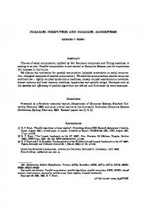
Chapter 5 field and offer more or less ready out–of–the–box cluster solutions for those groups that do not want to build their cluster from scratch. Beowulf clusters are mostly operated through the Linux operating system. Compared to the more integrated MIMD systems, often called MPP systems (Massive Parallel Processing) traditionally offered by supercomputer vendors, clusters still lack some of the tools and support to operate the system as effectively as possible. However, as clusters become on average both larger and more stable, there is a trend to operate them in similar mixed application environments as MPP systems. In the design of a cluster two important components are the network and the compute node. The speed of the network is very important in all but the most compute bound applications. The node configuration is often single or dual processor. A notable observation is that when using compute nodes with dual processors, which may be attractive from the point of view of cost–efficiency when using an expensive network or from compactness aspects, the performance can be severely damaged when more CPUs have to share on a common node memory. The bandwidth of the nodes is in this case not up to the demands of memory intensive applications. There is nowadays a wide range of communication networks available for clusters. Gigabit Ethernet is a widespread alternative, which is attractive for economic reasons, but has the drawback of a high latency (≈30–40 µs). Alternatively, there are for instance networks that operate from user space, like Myrinet [57], Infiniband [58] and SCI (Scalable Coherent Interface) [59]. The first two have reported bandwidths using ping–pong experiment in the order of 250 MB/s and 850 MB/s, respectively, and latency below 7µs. SCI delivers 320 MB/s in ping–pong test and latency under 3 µs. The latter solution is more costly but is nevertheless employed in some cluster configurations. The network speed as shown by these is more or less on par with some MPP systems. So, possibly apart from the speed of the processors and of the software that is provided by the vendors of MPP supercomputers, the distinction between clusters and MPPs becomes rather small and will certainly decrease in the coming years. The ranking of the 500 most powerful computer systems [60] worldwide clearly illustrates that MPP and cluster systems dominate the supercomputer arena today. Figure 6 presents the classification of system architecture on the top500 list since 1993. The classification is done using the following classes: o o o o o o
Constellation − Collection of SMPs SMP − Symmetric multi processing (shared memory systems) Single processor − Vector processor systems SIMD − Single Instruction Multiple Data systems MPP − Massive parallel processing systems Cluster − Distributed processing systems
With over 300 entries in the 26th list (Nov 2005) cluster is now the dominating architectural class of system. Looking at the trends since 1997 when the first cluster entered the list illustrates the impact cluster technology has had on the supercomputer evolution. Currently in the 1st position is the IBM system BlueGene/L installed at Lawrence Livermore National Laboratory in the U.S. with 131 000 processors delivering a Linpack performance of 281 TFlops. Of the top 10 ranked systems 8 are MPP systems and 2 are clusters. To enter the 26th list a performance of 1645 GFlops is required.
20
Parallel computer platforms 500 450 400 350
cons tellation
300
SMP
250
Single proc
200
SIMD
150
MPP Clus ter
100 50
04
03
02
05 20
20
20
01 20
20
99
98
97
96
95
94
00
20
19
19
19
19
19
19
19
93
0
Figure 6 Classification of systems in the top500 list. Source data from [60]. The largest systems dedicated to aerospace development are today located in Japan and the U.S. The National Aerospace Laboratory of Japan runs a 2304 processor Fujitsu system since 2003 delivering a Linpack performance of 5406 GFlops, currently at position 68. In the U.S Lockheed-Martin installed a 320 processor Xeon cluster in 2005 delivering 1710 GFlops. In Germany have Airbus, DLR and MTU Aero Engine recently installed clusters with performance ranging between 1200 and 1300 GFlops placing them just outside the 26th top500 list. Aerospace research centres in the U.S. have access to many of the major supercomputer installations, e.g. the BlueGene/L system at LLNL (1st rank) and the 10 000 processor SGI Altix installation at NASA Ames (4th rank).
5.2 EVALUATED SYSTEMS In this study, covering a time frame of six years, three generations of systems is studied. The early systems are a Cray T3E, a SGI Origin3000 and an early Siemens PC–cluster with 16 Intel Pentium III processors connected with SCI/Fast Ethernet. The more recent systems, Stokes, Maxwell, Monolith, Dunder and Darkstar, are all Beowulf systems based on Intel processors connected by SCI, Infiniband or Gigabit Ethernet. Most of the systems are designed and operated by National Supercomputer Centre at Linköping University, NSC1.
1
http://www.nsc.liu.se
21
Chapter 5 Table 2 Main features of evaluated systems. System Cray T3E
Processor
Network
DEC Cray-specific EV5 300MHz
Nodes Proc/node
Linpack (GFlops)
Service Top500 entry entry
268
1
117
1997-09
35
SGI Origin 3000
MIPS R14k 500MHz
ccNUMA
128
-
106.9
2001-03
-
Cluster Siemens
Intel PIII 850 MHz
SCI/Fast Ethernet
16
1
6.92
2000-02
-
Cluster- Intel Xeon 2.2 GHz Monolith
SCI/Fast Ethernet
200
2
1130
2002-12
51
ClusterMaxwell
Intel Xeon 2.4 GHz
SCI/Gigabit Ethernet
40
2
209
2003-02
-
Cluster Stokes
Intel P4 2.8 GHz
Gigabit Ethernet
32
1
98
2003-06
-
50
2
4402
2005-10
-
44
2
3802
2006-04
-
ClusterDunder
Intel Xeon 3.4 Infiniband/ GHz Gigabit Eth.
Cluster- Intel Xeon 3.4 GHz Darkstar
2
Estimated
22
Gigabit Ethernet
6 Performance measurements In parallel processing speedup and efficiency are two important measures of the quality of the parallel algorithm. Let Ts be the time to run the serial algorithm on one processor and Tp the time by a parallel algorithm on N processors then Speedup = SN = Ts / Tp and the efficiency of the parallel algorithm is given by Efficiency = EN = SN / N In the parallel algorithm as well as in the code implementation there are a number of factors limiting the speedup. Software Overhead – Even with a completely equivalent algorithm, software overhead arises in the parallel implementation, i.e. there are generally more lines of code to be executed in the parallel program than in the sequential program. Load Balancing – Speedup is generally limited by the speed of the slowest node. So an important consideration is to ensure that each node performs the same amount of work, i.e. the system is load balanced. Communication Overhead – Assuming that communication and calculation cannot be overlapped, any time spent communicating the data between processors directly degrades the speedup. Because of this, a goal in the design of a parallel algorithm is to make the grain size (relative amount of work done between synchronizations - communications) as large as possible, while keeping all the processors busy. The effect of communication on speedup is reduced, in relative terms, as the grain size increases. Amdahl’s Law – This states that the speedup of a parallel algorithm is effectively limited by the number of operations which must be performed sequentially. The performance evaluation is performed with the Edge code using inviscid flow modelling, given by the Euler equations, around the highly resolved Gripen fighter with external stores. A depiction of the surface grid used in this evaluation is shown in Figure 7. The case is geometrically complex with detailed external stores placed underneath the wings. A total of 3
23
Chapter 6 million points corresponding to approximately 18 million tetrahedral volume elements are needed for a full span model to adequately resolve the geometry and the flow features. A fully converged steady–state solution can be achieved in about 500 multi grid cycles. Computational models of this type and resolution are currently employed for configuration analysis, aerodynamic interference analysis and aerodynamic data generation. Often a large number of cases with different flow conditions are computed. In the present case the aerodynamic installation effect on the external stores is studied at transonic conditions with sideslip. Figure 7 also presents the pressure distribution on the upper side of the aircraft where a blue colour indicates low pressure regions.
Figure 7 Transonic flow around the Gripen fighter, surface mesh (left) and pressure distribution (right). A fixed size problem is used as the focus is on industrial applications and the intention is to reproduce the situation in the design process. When the problem is parallelized over more processors two parts will influence the performance results more than the other. Firstly the computation to communication ratio will decrease as the partitioning introduces new internal boundaries between domains. Both the total amount of data communicated as well as the number of messages increase. The communication pattern becomes more fragmented and the mean message size decreases. Secondly, when more processors are added the total amount of fast cache memory also increases. This means that a larger part of the total problem will reside in the cache with a subsequent performance gain. This is called cache effect and can result in a super linear speedup, i.e. higher speedup numbers than number of processors. The parallel performance is analyzed in terms of computational performance and parallel efficiency on five of the more recent clusters: Stokes, Maxwell, Monolith, Dunder and Darkstar listed in Table 2. The performance is measured on the entire code (excluding I/O), rather than detailed instrumentation of selected code sections. This is done by collecting the number of floating point operations through hardware counters and measuring the wall clock time for the parallel runs. The objective is here to demonstrate some of the key issues of parallel performance and the impact of the cluster configuration. For the type of algorithm used in this study, the load balancing and the communication overhead items are the most crucial to deal with to obtain good parallel performance. There are virtually no serial parts in the code and the software overhead is small compared to the other two. This makes the interconnecting network crucial in the design of a parallel system. Analyzing the communication behaviour of the code reveals that the communication quickly
24
Performance measurements gets latency bound. In this example the mean transfer time for messages is affected by latency already at 8 processors. Comparing the performance on clusters with different networks clearly verifies this. Clusters with low latency networks deliver good parallel efficiency also for a large number of processors as presented in Figure 8. In comparison, clusters with Gigabit Ethernet show a decrease in parallel efficiency already after 8 processors. This is in good correlation with where the message transfer gets latency dominated. With 256 processors on Monolith a total performance of 34 GFlops is achieved and using 64 processors on Dunder a performance of 26 GFlops is reached. The performance per processor differ a factor of 3. In comparison the theoretical processor speed only differs by 50 % and the remaining difference is mainly due to larger 2nd level cache on the Dunder system. This is also the reason behind the high efficiency values in Figure 8. Using a system that delivers more than 30 GFlops in application performance clearly affects the turn around time, which for this case is reduced to below 5 minutes. 40
1.3
1.2
Efficiency
GFlops
30
20
1.1
1 Dunder Xeon 3.4GHz Infiniband Darkstar Xeon 3.4GHz GigE Maxwell Xeon 2.4GHz SCI Maxwell Xeon 2.4GHz GigE Monolith Xeon 2.2GHz SCI Stokes P4 2.8GHz GigE
10
0
1
16
32
64
128 Number of processors
256
0.9
0.8
Dunder Xeon 3.4GHz Infiniband Darkstar Xeon 3.4GHz GigE Maxwell Xeon 2.4GHz SCI Maxwell Xeon 2.4GHz GigE 1
8
16
32 Number of processors
64
Figure 8 Parallel performance and parallel efficiency on different cluster configurations Much research has been devoted to load balancing and the finding in this study is that very good load balance can be obtained with a publicly available graph partitioner. In the simplest form an equal number of nodes are distributed between domains. When increasing the number of domains the communication (pattern and amount) also becomes important to balance between the domains. This is usually obtained by an additional constraint in the load balancing algorithm to balance (minimize) the number of boundary points. In this case a small performance gain is seen from 64 processors, plotted in Figure 9, using this additional constraint in the load balancing algorithm. The right figure presents the number of internal (communicated) boundary points per partition generated in the load balancing using k-Metis and p-Metis. The k-Metis algorithm generates partitions with less boundary points to communicate compared with p-Metis. This explains the improved performance above 32 processors for the k-Metis case. Why k-Metis fails to produce 2 and 4 partitions with less boundary points is not fully understood.
25
Chapter 6
300
20000
p-MeTiS k-MeTiS
k-MeTiS p-MeTiS
Number of connected points
250
Parallel Speedup
200
150
100
15000
10000
5000
50
0
0
32
64
128 Number of processors
256
0
1
2
4
8
32 16 Number of partitions
64
128
256
Figure 9 Parallel speedup and boundary points in partitions using p-Metis and k-Metis algorithms.
26
7 Summary of papers Paper I Two–equation turbulence models are introduced as high–end models in the aircraft design process. They deliver fairly good results for cruise conditions where the flow is attached or only moderately separated. For off–design cases where the flow shows larger separated regions they fail to predict the correct flow behaviour. Algebraic Reynolds Stress Models (EARSM) start to appear in the literature presenting improved results for aerospace applications. An EARSM is implemented in a structured multi block solver for evaluation of the performance on aircraft design applications. Computational results are compared with measurements for a transport wing and a transport aircraft configuration. In both cases significantly improved results are presented. The main reason for the improved flow prediction is the non-linear stress/strain relationship in the EARSM. Regions with adverse pressure gradients and separated flows are more realistically predicted compared with results from the linear two-equation model it is based upon (k-ω). The results clearly demonstrate that EARSM modelling is feasible in industrial applications and that the potential for increased accuracy in complex flow cases is high. The parallel implementation and load balancing strategy of the code is described and performance results from a number of parallel systems, including an early PC-cluster, are reported. Paper II With the introduction of PC-clusters cost-efficient high performance computer systems are more wide-spread. When designing a cluster there are a number of design choices to be made. The paper studies the impact on flow solver performance from a number of these alternatives as well as load balancing issues. A 3 million point unstructured CFD model is used as benchmark case. The two most important configuration components for high performance are the node configuration and the interconnecting network. Gigabit Ethernet is a cost-efficient alternative that performs well up to about 100 processors with current processor performance. With parallel application using more processors the need for low latency networks grow, even though with a significant cost increase. A way to reduce the number of connections, and thereby the cost, in the network is to use dual processor nodes. Dual processors have however limitations as the processors share the same memory bandwidth. In this study the
27
Chapter 7 performance loss using dual processors is 20 %. This is still a cost-efficient alternative with high performance networks. For clusters with Gigabit Ethernet single processor nodes are preferred unless the cluster size grow. Dual nodes can then be used to reduce network complexity and cost. Beside the hardware configuration, load balancing is also a significant issue for good parallel performance. Different load balancing algorithms are evaluated. Using moderate number of processors, up to 32, it is enough to balance only the number of grid points between the processors. Above 32 processors it is also important to keep the boundary points as few as possible and balance the communication load between the processors by using more advanced load balancing algorithms.
28
8 Conclusions This thesis has studied the industrial deployment of parallel computers as a mean to introduce more advanced flow modelling methods upstream in the aircraft design process. The most advanced flow modelling method used in aircraft design on a regular basis today is two–equation turbulence models. Introducing improved physical modelling through an EARSM significantly improved results are demonstrated on transport aircraft configurations. The non-linear stress/strain relationship in the EARSM performs superior to linear eddyviscosity models, especially in adverse gradient areas and close to separated regions often found in off-design conditions. The aerodynamic design is a long lead item in the aircraft development process. To reduce the turn around time, cost and development risks increased modelling capability must be introduced upstream in the development process. The main hurdle to introduce further advanced flow modelling at early stages is the turn around time for an analysis. This is usually addressed by using large parallel computers. With the recent success of Beowulf clusters cost–efficient high performing computers are made available to a larger community. By appropriate selection of the compute nodes and the network a cluster can be designed giving the best performance at a given cost on a chosen application suite. CFD solvers are memory intense applications and with dual processor nodes the memory bandwidth will be a limiting factor. Examples show a 20 % decrease in performance using dual nodes compared to single processor nodes. The cost difference between a dual node and two single nodes is roughly in the 20-25 % range. In typical design applications the communication is latency bound starting from approximately 8 processors. Obtaining good parallel performance for hundreds of processors will require a low latency network, which however is significantly more expansive than the Gigabit Ethernet alternative. Gigabit Ethernet is a cost-efficient alternative up to about 100 processors. Above that it performs poorly. The most appropriate cluster combination for this flow solver depends on the total size of the cluster. For a small cluster, up to 48 processors, single nodes with Gigabit Ethernet will be a cost-efficient solution. For larger clusters dual nodes are preferred. Depending on the parallelization strategy, number of processors per case, low latency networks can be required. The typical mesh size for a flow analysis around a complete aircraft is today in the range of 3–20 million points and this is usually parallelized on 20–80 processors. This will be well suited to run efficiently on cluster configurations with Gigabit Ethernet. Using more than 80–
29
Chapter 8 100 processors per case will require low latency networks for efficiency. This conclusion is today recognized by the aerospace community as exemplified by the largest cluster in the aerospace industry; a 464 processor (dual nodes) cluster with Gigabit Ethernet installed at Airbus in Germany in 2005.
30
9 Outlook The use of Computational Fluid Dynamics and numerical multidisciplinary simulation and optimization will continue to grow in the aerospace industry. The goal of significantly reducing the development cost and time to market of a new aircraft will require an integrated design environment and use of the virtual product concept by further exploring the potential of computer simulations. To implement this vision several improvements are needed in the area of flow simulations. Turn around time: To use computational aerodynamics in the integrated design environment requires short turn around time for CFD simulations. Today the time needed to go from a CAD geometry to an Euler or a Navier–Stokes solution is several orders too large for use in the virtual product concept although parallel processing is common practice. Routine use of transient simulations, increasing grid resolution, generation of complete data sets (an upper bound of 200 thousand cases is mentioned by Jou [5]) will require CFD simulation time to be reduced at least 1–2 orders of magnitude. Improved solution schemes, massively parallel computers and improved implementation on these machines are all needed to meet this challenge. For instance, today most CFD codes achieve only 5–10 % of the theoretical performance of an x86–type processor. Better implementations and improved compilers can substantially improve the performance also on present parallel systems. Apart from the reduction in CPU time, numerical methods must be robust enough to avoid time– consuming tuning of parameters in order to obtain a solution. This is crucial for a broad acceptance of CFD simulations by the aircraft design engineers, who will likely not be CFD experts. Increasing geometrical complexity and resolution will also affect the pre–processing and post–processing. The pre–processing (mesh generation) tools have improved over the last years reducing the mesh generation time for basic configurations significantly. However, there are still unresolved problems with fluid/structure coupling for transient simulation involving moving or deforming surfaces, e.g. control–surface movements. The re–import of optimized shapes into CAD systems also needs to be resolved. Post–processing is already today a time consuming task. In the future, the number of grid points will increase together with the number of computed cases and large transient simulations will become routine. Improvements in visualization tools are needed with fast data extraction tools, feature detection tools and better man–machine interface. Exploring results from maybe thousands of simulations will require automated tools that extract relevant features for further processing. Aerodynamic simulation results will primarily go into three
31
Chapter 9 different databases covering; performance, stability/control characteristics, and critical loads, thus providing the interface to other disciplines in the design process. Physical modelling: Bringing down the turn around time of CFD simulations is by itself not enough to reach the virtual product vision. The simulations must also improve in the predictions of the flow physics to capture the correct properties and functions of the product. Some of the challenging applications that need to be resolved in the coming years are outlined below. Navier–Stokes simulations are today performed on wing–body–pylon–nacelle configurations at design conditions (cruise conditions) where separated regions are either small or non– existing. These computations provide the designer with valuable information about load distributions vital for the structural design. Often the critical design loads are found in off– design conditions when the separated regions of the flow become more dominating. Thus an effective code must accurately capture all the important phenomena in separated flow, i.e. wall shear layers, free shear layers and vortices. Engine integration is another important task in aircraft design. The development of ultra– high–bypass aero–engines with superior efficiency and low noise and emission presents the problem of the engines’ sheer size in relation to the aircraft. The effect of varying the engine positions, shape and size of nacelles and pylons, calculation of the jet effects and shed wakes over the associated airframe surfaces in cruise and high–lift configurations and speeds need to be investigated. Such advanced simulations, especially when coupled with optimization, will become invaluable aids to airframe and engine manufacturers in developing future products. The friction drag of a commercial aircraft amounts to more than 50% of the total drag, and therefore any means of reducing it translates into clear economical benefits in term of fuel savings, extended operational range and/or increased payload. Challenging areas for research are drag and thrust analysis of new aircraft, drag prediction of new wings and bodies, and the optimization of tail flow. The overall accuracy and reliability in the prediction of drag polar, drag rise in transonic flight and drag reduction technologies is a research topic currently of much interest. The simulation of unsteady phenomena, whether a pure aerodynamic phenomenon, e.g. dynamic stall or transonic buffeting, or a fluid–structural phenomena as flutter or a fluid– solid body mechanics problem as store separation, is today very challenging. The computational effort is substantial making simulations far from routine. There are also deficiencies in the present physical models to properly deal with turbulence etc. To summarize, the challenge for the future is to enable the designer to base his decisions, with some degree of confidence, on simulations of the aerodynamic response of a complete aircraft configuration in manoeuvres that predicts maximum usable lift, the onset of buffet, off–design dynamic loads, and noise generation.
32
10 Acknowledgments This licentiate thesis is the result of work carried out at the Department of Aeronautical Engineering at Saab Aerosystems and National Supercomputer Centre (NSC) at Linköping University between December 2000 and March 2006. Part of the work was performed within the EC–project AVTAC–Advanced Viscous Flow Simulation Tools for Complete Civil Transport Aircraft Design (Contr. No. BRPR CT97–0555). Computer resources were supplied both by Saab Aerosystems and NSC. I am grateful for the support and feedback from colleagues at Saab and NSC throughout the process. I am likewise grateful to the Edge-group at FOI for fruitful discussion on Edgerelated issues. Last but not least thanks goes to my supervisors Professor Dan Loyd and Professor Matts Karlsson who has encouraged me to complete this work.
33
34
11 Bibliography 1.
E.H. Hirschel, “Towards the virtual product in aircraft design?”, Proceedings of NDF 2000–Towards a New Fluid Dynamics with its Challenges in Aerospace Engineering, CNRS, Paris, November, 2000. In: M. Champion, J. Periaux, O. Pironneau, P. Thomas, (eds.), NFD2000: Towards a new fluid dynamics. CIMNE Handbooks on Theory and Engineering Applications of Computational Methods, Barcelona 2000.
2.
P. Rostand, “New Generation Aerodynamic and Multidisciplinary Design Methods for the FALCON Business Jets: Application to the F7X”, AIAA Paper 2005-5083, 2005.
3.
J.B. Vos, A. Rizzi, D. Darracq and E.H. Hirschel, “Navier-Stokes solvers in European aircraft design”, Progress in Aerospace Sciences, No. 38, 2002, pp. 601697.
4.
J. Szodruch and R. Hilbig, “Building the future aircraft design for the next century”, AIAA Paper 98-0135, 1998.
5.
W-H. Jou. “A systems approach to CFD code development”, In Proceedings ICAS 1998 Congress, 1998.
6.
A. Jameson, “The present status, challenges, and future developments in computational fluid dynamics”, In: Progress and Challenges in CFD Methods and Algorithms, AGARD-CP-578, 1996.
7.
P. Raj, “CFD at a crossroads: An industry perspective”, In: Frontiers of Computational Fluid Dynamics 1998, D.A. Caughey and M.M. Hafez (eds.) 1998.
8.
S.S. Samant, J.E. Bussoletti, F.T. Johnson, R.H. Burkhart, B.L. Everson, R.G. Melvin, D.P. Young, L.L. Erickson, M.D. Madson and A.C. Woo, “TRANAIR: A Computer Code for Transonic Analysis of Arbitrary Configuration”, AIAA Paper 870034, 1987.
9.
D.H. Bailey, T.V. Harris, R. der Wigngaart, W. Saphir, A. Woo and M. Yarrow, “The NAS Parallel Benchmark 2.0,” Technical Report NAS-95-020, NASA Ames Research Center, 1995.
35
Chapter 11 10. A. Jameson, W. Schmidt and E. Turkel, "Numerical solution of the Euler equations by finite volume methods using Runge-Kutta time stepping schemes." AIAA Paper 81-1259, June 1981. 11. J. Dongarra, G.A. Geist, R. Manchek and V.S. Sunderam, “Integrated PVM framework supports heterogeneous network computing”, Computers in Physics, Vol. 7, 1993, pp. 166-174. 12. MPI Forum, “MPI: A Messages-Passing Interface Standard”, International Journal of Supercomputing Applications, Vol. 8, 1994. 13. OpenMP Forum, Fortran Language Specification, Web site:www.openmp.org/ (cited 2006-04-04). 14. T.L. Sterling, J. Salmon, D.J. Becker and D.F. Savarese, “How to build a Beowulf”, Cambridge, MA, MIT Press, 1999. 15. E.H. Hirschel, “Present and future aerodynamic process technologies at DASA military aircraft”, Proceedings ERCOFTAC Industrial Technology Topic Meeting, October 1999. 16. A. Gould, J-C. Courty, M. Sillén, E. Elsholz and A. Abbas, “The AVTAC Project – a Review of European Aerospace CFD”, In Proceedings ECCOMAS 2000, 2000. 17. P. Aumann, H. Barnewitz, H. Schwarten, K. Becker, R. Heinrich, B. Roll, M. Galle, N. Kroll, Th. Gerhold, D. Schwamborn and M. Franke, “MEGAFLOW: Parallel complete aircraft CFD”, Parallel Computing, Vol. 27, 2001, pp. 415-440. 18. J.W. van der Burg, K.M.J. de Cook, T. Berglind, W. Fritz, G. Kretzschmar, N. Kroll, D. Schwamborn and M. Sillén, “A joint European initiative to develop hybrid grid based CFD technology for inviscid and viscous flow computations applicable to geometrically complex aircraft”, In Proceedings of the CEAS European Aerodynamics Conference, 10-12 June 2002. 19. A.J. Peace, “Maximising the impact of CFD in the design office: ARA’s role”, The Aeronautical Journal, Dec. 2002, pp. 675-685. 20. P. Raj, “Aircraft design in the 21st century: implications for design methods”, AIAA Paper 98-2895, 1998. 21. A. Jameson, “Computational Transonics”, Comm. Pure Appl. Math., Vol. 41, 1988, pp. 507-549. 22. M. Sillén, “Flow Simulation around the Exact Canopy Geometry of the Space plane HERMES”, AIAA Paper 93-5025, Dec. 1993. 23. M. Sillén, “Sideslip Aerodynamics for Hytex Space Vehicle”, Proceedings of the 1996 ICAS Conference, Paper ICAS- 96-2.6.3, Sept. 1996. 24. M. Sillén, “Investigation of Base Flow on a Space Rocket with Plumes”, AIAA Paper 98-1599, 1998.
36
Bibliography 25. M. Sillén, “Advanced Flow Simulation Methods in Aircraft Design”, Proceedings RRDPAE2000 Conference, Warsaw, Poland, 2000. 26. B. Arlinger, T. Larsson, P. Lötstedt and M. Sillén, “Some recent CFD developments and applications at Saab”, Frontiers of Computational Fluid Dynamics 1994, D.A. Caughey and M. Hafez (eds.), John Wiley and Sons Ltd, 1994, pp. 509-527. 27. P. Lötstedt and M. Sillén “Multigrid multiblock solver of the stationary Euler and Navier-Stokes equations II”, Report L-0-1 R164, Saab AB, Linköping, Sweden, 1996. 28. A. Ålund, P. Lötstedt and M. Sillén, “Parallel single and multigrid solution of industrial compressible flow problems”, Computers & Fluids, Vol. 26, No. 7, 1997, pp. 775-791. 29. P. Eliasson, “EDGE, a Navier-Stokes solver for unstructured grids”, Proceedings of the Finite Volumes for Complex Applications III, ISBN 1 9039 9634 1, 2003, pp. 527-534. 30. B.S. Baldwin, H. Lomax, “Thin layer approximation and algebraic model for separated flows”, AIAA Paper 78-257, 1978. 31. L. Prandtl, ”Uber ein neues Formelsystem fur die ausgebildete Turbulenz”, Nacr. Akad. Wiss. Göttingen, Math-Phys. Kl., 1945, pp. 6-9. 32. P.R. Spalart and S.R. Allmaras, "A one-equation turbulence model for aerodynamic flows", AIAA Paper 92-439, 1992. 33. D.C. Wilcox, “Turbulence modeling for CFD”, DCW Industries Inc., La Canada, California, 1993. 34. J. Kok, “Resolving the dependency on free-stream values for the k-ω turbulence model”, AIAA Journal, Vol. 38, No. 7, 2000, pp. 1292-1295. 35. S. Wallin and A.V. Johansson, “An explicit algebraic Reynolds stress model for incompressible and compressible turbulent flows”, Journal Fluid Mechanics, Vol. 403, 2000, pp. 89-132. 36. T.B. Gatski, C.G. Speziale, “A new algebraic relation for calculating the Reynolds stresses”, Journal of Fluid Mechanics, Vol. 254, 1993, pp. 59-78. 37. P.R. Spalart, W.-J. Jou, M. Strelets, and S.R. Allmaras, “Comments on the feasibility of LES for wings and on the hybrid RANS/LES approach, Advances in DNS/LES”, 1st AFOSR Intl. Conf on DNS/LES, Greyden Press. 1997, pp. 137-148. 38. M.A. Leschziner, D. Drikakis, “Turbulence modeling and turbulent-flow computation in aeronautics”, The Aeronatical Journal, July 2002, pp.349-384. 39. M. Rakowitz, M. Sutcliffe, B. Eisfeld, D. Schwamborn, H. Bleecke and J. Fassbender, “Structured and Unstructured Computations on the DLR-F4 Wing-Body Configuration”, AIAA Paper 2002-837, 2002.
37
Chapter 11 40. P. Lötstedt, A. Ålund, “Multigrid solution of the Euler and Navier-Stokes equations on a workstation cluster in an industrial environment”, ITM Report No 1994:3, Chalmers, Sweden, 1994. 41. M. Sillén and P. Weinerfelt, “Industrial experience of CFD on parallel computers”, In ECCOMAS´98 Conference Proceedings, Vol. 2, Papailiou, Tsahalis, Periaux and Knörzer (eds), John Wiley & Sons, 1998, pp.754-759. 42. A. Ålund, P. Lötstedt and M. Sillén, “Parallel solution of industrial compressible flow problems with static load balancing”, In: Parallel Computational Fluid Dynamics – Algorithms and Results using Advanced Computers, Schiano, Ecer, Periaux, Satufuka (eds), North-Holland, ISBN 0 444 82327 1, 1997, pp. 336-351. 43. G. Karypis and V. Kumar, “Analysis of Multilevel Graph Partitioning”, Technical Report 95-037, Univ. of Minnesota, 1995. 44. D.J. Mavriplis, “Parallel performance investigation of an unstructured mesh NavierStokes solver”, The International Journal of High Performance Computing Applications, Vol. 16, No. 4, 2002, pp. 395-407. 45. R.H. Bush, G.D. Tower and C.E. Towne, “WIND: The production flow solver of the NPARC alliance”, AIAA Paper 98-0935, Jan. 1998. 46. N.T. Frink, “Tetrahedral unstructured Navier-Stokes method for turbulent flows”, AIAA Journal, Vol. 36, No. 11, 1998, pp. 1975-1982. 47. W.Z. Strang, R.F. Tomaro and M.J. Grismer. ”The defining methods of COBALT60: a parallel implicit unstructured Euler/Navier–Stokes flow solver”, AIAA Paper 990786, 1999. 48. D.J. Mavriplis, “Three-dimensional viscous flow analysis for high-lift configurations using a parallel unstructured multigrid solver”, SAE Paper 1999-01-5558 presented at the SAE World Aviation Congress, San Fransisco, CA, Oct-19-21, 1999. 49. S.E. Rogers, K. Roth, H.V. Cao, J.P. Slotnick, M. Whitlock, S.M. Nash and M.D. Baker, “Computation of viscous flow for a Boeing 777 aircraft in landing configuration”, Journal of Aircraft, Vol. 48, No. 6, 2001, pp. 1060-1068. 50. J.R. Forsythe and S.H. Woodson, “Unsteady Computation of Abrupt Wing Stall using Detached-Eddy Simulation”, Journal of Aircraft, Vol. 42, No. 3, 2005, pp. 606616. 51. I. Mary and P. Sagaut, “Large eddy simulation of flow around an airfoil”, AIAA Paper 2001-2559, 2001. 52. F. Chalot, B. Marquez, M. Ravachol, F. Ducros, F. Nicoud and T. Poinsot, “A consistent finite element approach to large eddy simulation”, AIAA Paper 19982652, 1998. 53. M.S. Fisher, M. Mani and D. Stookesberry, “Parallel Processing with the Wind CFD Code at Boeing”, Parallel Computing, Vol. 27, 2001, pp. 441-456.
38
Bibliography 54. C. Gacherieu, E. Chaput and L. Tourette, "Navier-Stokes for design of transport aircraft using parallel computing.", In Proceedings 3rd ECCOMAS Computational Fluid Dynamics Conference, 1996. 55. S. Peigin B. Epstein, T. Rubin and S. Seror, “Parallel large scale high accuracy Navier-Stokes computations on distributed memory clusters”, The Journal of Supercomputing, Vol. 27, 2004, pp. 49-68. 56. R. Chandra, L. Dagum, D. Kohr, D. Maydan, J. McDonald and R. Menon, “Parallel Programming in OpenMP”, Morgan Kaufmann Publishers Inc., January 2001. 57. N.J. Boden, D. Cohen, R.E. Felderman, A.E. Kulawik, C.L. Seitz, J.N. Seizovic and S. Wen-King, “Myrinet -- A Gigabit-per-second Local Area Network”, IEEE Micro, Vol. 15, No. 1, Jan. 1995, pp. 29-36. 58. T. Shanley, “Infiniband Network Architecture”, Addison-Wesley, November 2002. 59. D.V. James, A.T. Laundrie, S. Gjessing and G.S. Sohi, “Scalable Coherent Interface”, IEEE Computer, Vol. 23, No. 6, 1990, pp. 74-77. 60. Top500 Supercomputer sites, webpage: http://www.top500.org (cited 2006-04-04).
39