ornl/tm-12986 performance of parallel computers for ... - CiteSeerX

ORNL/TM-12986 Computer Science and Mathematics Division Mathematical Sciences Section

PERFORMANCE OF PARALLEL COMPUTERS FOR SPECTRAL ATMOSPHERIC MODELS Ian T. Foster  Brian Toonen  Patrick H. Worley y 

Argonne National Laboratory Mathematics and Computer Science Division Argonne, IL 60439-4801

y

Oak Ridge National Laboratory Mathematical Sciences Section P. O. Box 2008 Oak Ridge, TN 37831-6367

Date Published: April, 1995 Research was supported by the Atmospheric and Climate Research Division of the Oce of Energy Research, U.S. Department of Energy Prepared by the Oak Ridge National Laboratory Oak Ridge, Tennessee 37831 managed by Martin Marietta Energy Systems, Inc. for the U.S. DEPARTMENT OF ENERGY under Contract No. DE-AC05-84OR21400

Contents 1 Introduction : : : : : : : : : : : : 2 Background : : : : : : : : : : : : 2.1 Parallel Computers : : : : : 2.2 Spectral Transform Method 3 Experimental Method : : : : : : 3.1 The PSTSWM Testbed : : 3.2 Experimental Technique : : 3.3 Target Computers : : : : : 4 Results : : : : : : : : : : : : : : : 5 Discussion : : : : : : : : : : : : : 5.1 Single-Node Performance : 5.2 Parallel Performance : : : : 5.3 Precision : : : : : : : : : : : 5.4 Algorithms : : : : : : : : : 5.5 Price Performance : : : : : 5.6 Coding Style : : : : : : : : 6 Conclusions : : : : : : : : : : : :

: : : : : : : : : : : : : : : : :

: : : : : : : : : : : : : : : : :

: : : : : : : : : : : : : : : : :

: : : : : : : : : : : : : : : : :

: : : : : : : : : : : : : : : : :

: : : : : : : : : : : : : : : : :

: : : : : : : : : : : : : : : : :

- iii -

: : : : : : : : : : : : : : : : :

: : : : : : : : : : : : : : : : :

: : : : : : : : : : : : : : : : :

: : : : : : : : : : : : : : : : :

: : : : : : : : : : : : : : : : :

: : : : : : : : : : : : : : : : :

: : : : : : : : : : : : : : : : :

: : : : : : : : : : : : : : : : :

: : : : : : : : : : : : : : : : :

: : : : : : : : : : : : : : : : :

: : : : : : : : : : : : : : : : :

: : : : : : : : : : : : : : : : :

: : : : : : : : : : : : : : : : :

: : : : : : : : : : : : : : : : :

: : : : : : : : : : : : : : : : :

: : : : : : : : : : : : : : : : :

: : : : : : : : : : : : : : : : :

: : : : : : : : : : : : : : : : :

: : : : : : : : : : : : : : : : :

: : : : : : : : : : : : : : : : :

: : : : : : : : : : : : : : : : :

: : : : : : : : : : : : : : : : :

1 1 1 2 6 6 7 8 11 17 17 18 19 19 22 22 22

PERFORMANCE OF PARALLEL COMPUTERS FOR SPECTRAL ATMOSPHERIC MODELS Ian T. Foster Brian Toonen Patrick H. Worley

Abstract Massively parallel processing (MPP) computer systems use high-speed interconnection networks to link hundreds or thousands of RISC microprocessors. With each microprocessor having a peak performance of 100 M ops/sec or more, there is at least the possibility of achieving very high performance. However, the question of exactly how to achieve this performance remains unanswered. MPP systems and vector multiprocessors require very dierent coding styles. Dierent MPP systems have widely varying architectures and performance characteristics. For most problems, a range of dierent parallel algorithms is possible, again with varying performance characteristics. In this paper, we provide a detailed, fair evaluation of MPP performance for a weather and climate modeling application. Using a specially designed spectral transform code, we study performance on three dierent MPP systems: Intel Paragon, IBM SP2, and Cray T3D. We take great care to control for performance dierences due to varying algorithmic characteristics. The results yield insights into MPP performance characteristics, parallel spectral transform algorithms, and coding style for MPP systems. We conclude that it is possible to construct parallel models that achieve multi-G op/sec performance on a range of MPPs, if the models are constructed to allow run-time selection of appropriate algorithms.

-v-

1. Introduction In recent years, a number of computer vendors have produced supercomputers based on a massively parallel processing (MPP) architecture. These computers have been shown to be competitive in performance with conventional vector supercomputers for many applications (Fox, Williams, and Messina 1994). Since spectral weather and climate models are heavy users of vector supercomputers, it is interesting to determine how these models perform on MPPs and which MPPs are best suited to the execution of spectral models. The benchmarking of MPPs is complicated by the fact that dierent algorithms may be more ecient on dierent MPP systems. Hence, a comprehensive benchmarking eort must answer two related questions: which algorithm is most ecient on each computer and how do the most ecient algorithms compare on dierent computers. In general, these are dicult questions to answer because of the high cost associated with implementing and evaluating a range of dierent parallel algorithms on each MPP platform. In a recent study, we developed a testbed code called PSTSWM (Worley and Foster 1994) that incorporated a wide range of parallel spectral transform algorithms. Studies with this testbed con rm that the performance of dierent algorithms can vary signi cantly from computer to computer and that no single algorithm is optimal on all platforms (Foster and Worley 1994). Availability of this testbed makes it feasible to perform a comprehensive and fair benchmarking exercise of MPP platforms for spectral transform codes. We report here the results of this exercise, presenting benchmark results for the Intel Paragon, the IBM SP2, and the Cray T3D. The paper is structured as follows. First, we provide some background information on parallel computing, the spectral transform method, and parallel algorithms for the spectral transform. Then, we describe our experimental method, providing details of both the PSTSWM code and the parallel computers on which experiments were performed. In Section 4 we present our results; in Section 5 we discuss their signi cance. We conclude with a summary of our ndings.

2. Background We rst provide some background information on parallel computer architecture and on the spectral transform method used in the testbed code.

2.1. Parallel Computers In this paper, we focus on distributed-memory MIMD (multiple instruction, multiple data) computers, or multicomputers. In these computers, individual processors work independently of each other and exchange data via an interconnection network. Computers in this class include the Intel Paragon, IBM SP2, Cray T3D, Meiko CS2, and nCUBE/2. The performance of a multicomputer depends on more than just the oating point speed of its

-2component processors. Since processors must coordinate their activities and exchange data, the cost of sending messages must also be considered. The cost of transmitting a message between any two processors can be represented with two major parameters: the message startup time (ts ), which represents the xed overhead for any communication request, and the transfer time per byte (tb ), which includes any copying of the message between user and system buers, as well as the physical bandwidth of the communication channel. In this model, the time required to send a message of size B bytes to a processor is then ts + tb B: This expression is approximate, since contention on the network or for local memory access can increase either parameter, and on some computers the full bandwidth is realized only for larger s. The importance of this model is in parallel algorithm design and analysis: on some multicomputers, ts is very large and the number of messages must be minimized; on others, ts is small and the volume of data (s) moved between processors during execution determines the communication costs. An ecient parallel algorithm minimizes both communication costs and load imbalance, while supporting code structures that maximize single processor performance. A load imbalance occurs when some processors are idle while others are computing. To avoid this situation, computation is partitioned so that each processor has approximately the same amount of work to do in each phase of the computation. This partitioning is often achieved by dividing the data that is to be operated on, and making each processor responsible for computation on its piece of the data. An additional constraint on the choice of partitioning scheme is that it should minimize the amount of nonlocal data required at each processor, and hence the amount of communication required to transfer this data. Given the number of variables mentioned above, it should not be surprising that there are often multiple viable parallel algorithms for a particular problem, with dierent performance characteristics in dierent situations.

2.2. Spectral Transform Method A variety of numerical methods|e.g., nite dierence, semi-Lagrangian, and spectral transform| have been used in computer simulations of the atmospheric circulation (Browning, Hack, and Swarztrauber 1989). Of these, nite dierence methods are the easiest to parallelize because of their high degree of locality in data reference. Semi-Lagrangian methods introduce additional complexity because of their nonlocal and time-varying access patterns (Williamson and Rasch 1989). Spectral transform methods have important computational advantages (Bourke 1972), but are in many respects the most dicult to parallelize eciently, because of their highly nonlocal communication patterns. In this study, we used the spectral transform method to solve the nonlinear shallow water equations on the sphere. The resulting numerical algorithm is very similar to that used in the

-3NCAR Community Climate Model to handle the horizontal component of the primitive equations (Hack et al. 1992). For concreteness, we rst describe the shallow water equations in the form that we solve using the spectral transform method. We then describe the spectral transform method for these equations. We nish with a brief description of the parallel algorithms being examined.

Shallow Water Equations. The shallow water equations on a sphere consist of equations for the conservation of momentum and the conservation of mass. Let i, j, and k denote unit vectors in spherical geometry; V denote the horizontal velocity, V = iu+ jv;  denote the geopotential; and f denote the Coriolis term. Then the horizontal momentum and mass continuity equations can be written as (Washington and Parkinson 1986) DV = ?f k  V ? r Dt D = ?r
V; Dt where the substantial derivative is given by @ D Dt ( )  @t ( ) + V
r( ) :

(1)

(2)

The spectral transform method does not solve these equations directly; rather, it uses a stream function-vorticity formulation in order to work with scalar elds. De ne the vorticity  and the horizontal divergence  by  = f + k
(r  V)  = r
V : To avoid the singularity in velocity at the poles, let  represent latitude and rede ne the horizontal velocity components as ( U ; V ) = V cos  : After some manipulation, the equations can be written in the form 1@ @ @ = ? 1 @t a(1 ? 2 ) @ (U) ? a @ (V ) @ = + 1 @ (V ) ? 1 @ (U) ? r2  + U 2 + V 2  @t a(1 ? 2 ) @ a @ 2(1 ? 2 ) 1@ @ = ? 1 @  @t a(1 ? 2 ) @ (U) ? a @ (V ) ?  :

(3) (4) (5)

Here a is the radius of the sphere, the independent variables  and  denote longitude and

-4sin , respectively, and  is now a perturbation from a constant average geopotential  . Finally, U and V can be represented in terms of  and  through two auxiliary equations expressed in terms of a scalar stream function and a velocity potential : 1 ? 2 @ U = a1 @ ? @ a @ 2 @ ; V = a1 @@ + 1 ?a  @

(7)

 = r2 + f  = r2  :

(8) (9)

(6)

where

In the spectral transform method, we solve Eqs. 3{5 for , , and , and use Eqs. 6{9 to calculate U and V .

Spectral Transform Method. In the spectral transform method, elds are transformed at each timestep between the physical domain, where the physical forces are calculated, and the spectral domain, where the horizontal terms of the dierential equation are evaluated. The physical domain is represented by a computationally uniform physical grid with coordinates (i ; j ), where 1  i  I and 1  j  J. Fields in the spectral domain are represented as sets of spectral coecients. The spectral representation of a scalar eld  is de ned by a truncated expansion in terms of the spherical harmonic functions fPnm ()eim g: (; ) = where

(m) M NX X

m=?M n=jmj

nm Pnm ()eim ;

 Z 1  1 Z 2 ?im d P m ()d (; )e n 2 0 Z?11   m ()Pnm ()d :

nm =

p

?1

(10)

Here i = ?1,  = sin ,  is latitude,  is longitude, m is the wave number or Fourier mode, and Pnm () is the associated Legendre function. M and N(m) specify the form of the truncation of coecients, as discussed below. Note that Eq. 3{5 contain both linear and quadratic terms. In order to prevent aliasing of the quadratic terms in the numerical approximation, the number of points in both directions

-5is chosen to be larger than the degree of the expansion. For example, the number of points in longitude I  3M + 1, where M is the highest Fourier wave number. Thus, we use a standard discrete Fourier transform but truncate its output to 2M + 1 values. The number of terms in the Legendre expansions is similarly truncated. For this study, we restricted our experiments to triangular truncations, that is, N(m) = M. As Eq. 10 suggests, the spectral transform can be implemented by a Fourier transform followed by a Legendre transform. The Legendre transform (LT) requires the computation of an integral, which is approximated by using Gaussian quadrature. Thus, the latitude points j are picked as Gaussian grid points. (The longitude points i are ordinarily picked as uniformly spaced to simplify the Fourier transforms.) The Fourier transform, which can be implemented with the fast Fourier transform (FFT), operates on each grid space latitude independently to produce a set of intermediate quantities. The Legendre transform then operates on each column of the intermediate array independently to produce the spectral coecients. (The inverse spectral transform operates in the reverse sequence.) In our shallow water equation code (Hack and Jakob 1992), each timestep begins by calculating the nonlinear terms U, V , U, V , and +(U 2 +V 2)=(2(1 ? 2 )) on the physical grid. Next, the nonlinear terms and the state variables , , and  are Fourier transformed. The forward Legendre transforms of these elds are then combined with the calculation of the tendencies used in advancing , , and  in time (essentially evaluating the right-hand sides of Eqs. 3{5) and the rst step of the time update. This approach decreases the cost, when compared with calculating transforms individually and then calculating the tendencies, and generates spectral coecients for only three elds instead of eight. Next, the time updates of , , and  on the spectral grid are completed. Finally, the inverse Legendre transforms of , , and  are combined with the calculation of the elds U and V (solving Eqs. 6{9), followed by inverse Fourier transforms of these ve elds.

Parallel Spectral Transform Method. In this study, all parallel algorithms are based on

decomposing the dierent computational spaces onto a logical two-dimensional grid of processors, P = PX  PY . As will be described in the next section, a ctitious vertical dimension has been added to the shallow water model. In each space, two of the domain dimensions are decomposed across the two axes of the processor grid, leaving one domain dimension undecomposed. All parallel algorithms begin with the vertical dimension undecomposed in the physical domain, since, in full atmospheric models, the columnar physics are unlikely to be eciently parallelizable (Foster and Toonen 1994). Two basic types of parallel algorithm are examined: transpose and distributed. In a transpose algorithm, the decomposition is \rotated" before a transform begins to ensure that all data needed to compute a particular transform is local to a single processor. Thus, for example, before computing the Fourier transform, the longitude dimension is \undecomposed," and the vertical dimension is decomposed, allowing each processor to independently compute the Fourier transforms corresponding to the latitudes and vertical layers assigned to it. In a dis-

-6tributed algorithm, the original decomposition of the domain is retained, and communication is performed to allow the processors to cooperate in the calculation of a transform. For example, in a distributed Fourier transform all processors in a row of the processor grid cooperate to compute the Fourier transforms corresponding to the latitudes and vertical layers associated with that processor row.

3. Experimental Method We rst outline the structure of the PSTSWM testbed code, the experiments that were performed during the benchmarking exercise, and the computers on which benchmarks were performed.

3.1. The PSTSWM Testbed A number of researchers have investigated parallel algorithms for the spectral transform algorithm used in atmospheric circulation models. A variety of dierent parallel algorithms have been proposed (Dent 1990; Gartel, Joppich, and Schuller 1993; Loft and Sato 1993; Pelz and Stern 1993; Walker, Worley, and Drake 1992; Worley and Drake 1992), and some qualitative comparisons have been reported (Foster, Gropp, and Stevens 1992; Kauranne and Barros 1993; Foster and Worley 1993). However, until recently no detailed quantitative comparisons of the dierent approaches had been attempted. To permit a fair comparison of the suitability of the various algorithms, we have incorporated them into a single testbed code called PSTSWM, for parallel spectral transform shallow water model (Foster and Worley 1994; Worley and Foster 1994). PSTSWM is a message-passing parallel implementation of the sequential Fortran code STSWM (Hack and Jakob 1992). STSWM uses the spectral transform method to solve the nonlinear shallow water equations on a rotating sphere; its data structures and implementation are based directly on equivalent structures and algorithms in CCM2 (Hack et al. 1992), the Community Climate Model developed at the National Center for Atmospheric Research. PSTSWM diers from STSWM in one major respect: vertical levels have been added to permit a fair evaluation of transpose-based parallel algorithms. This is necessary because in a onelayer model, a transpose algorithm reduces to a one-dimensional decomposition of each grid and hence can utilize only a small number of processors. The addition of vertical levels also has the advantage of modeling more accurately the granularity of the dynamics computation in atmospheric models. In all other respects we have changed the algorithmic aspects of STSWM as little as possible. In particular, we did not change loop and array index ordering, and the serial performance of the code is consistent with that demonstrated by CCM2. PSTSWM is structured so that a variety of dierent algorithms can be selected by run-time parameters. Both the fast Fourier transform (FFT) and the Legendre transform (LT) that make up the spectral transform can be computed by using several dierent distributed algorithms and transpose algorithms. Runtime parameters also select from among a range of variants of

-7each of these major algorithms. All parallel algorithms were carefully implemented, eliminating unnecessary buer copying and exploiting our knowledge of the context in which they are called. At the present time, this allows us to achieve better performance than can be achieved by calling available vendor-supplied routines. Hence, it provides a fairer test of the parallel algorithms. While we have attempted to make PSTSWM as representative of full spectral weather and climate models as possible, it diers from such models in two important respects. First, we do not incorporate the vertical coupling in spectral space that is introduced by the use of a semi-implicit solver; this coupling is unnatural in a shallow water setting. We do not expect the interprocessor communication required to support the vertical coupling to contribute signi cantly to total costs because it involves only a single spectral space eld. This expectation has been veri ed empirically in the parallel version of the Integrated Forecast System developed at the European Centre for Medium-Range Weather Forecasting (Barros 1994). Second, PSTSWM does not incorporate realistic physics or the semi-Lagrangian transport (SLT) mechanisms that are used in many modern weather and climate models. To a signi cant degree, the parallel algorithm decisions and performance for the spectral transform method are orthogonal to those for physics and SLT, and the performance measurements and analysis reported here are valid, if not sucient for predicting performance of full models.

3.2. Experimental Technique We performed experiments for a range of horizontal and vertical resolutions, as summarized in Table 1. (Horizontal resolution is speci ed in terms of both spectral truncation and physical grid size, and the spectral truncation speci cation is pre xed by a \T," to denote a triangular truncation.) This range of resolutions was considered necessary because there is little agreement on standard resolutions and because the performance of dierent parallel algorithms can vary signi cantly depending on the number of vertical levels. The highest vertical resolutions in the T42 and T85 models are intended to be representative of resolutions used in stratospheric models. All experiments involved a ve-day simulation using the performance benchmark proposed by Williamson et al. (1992): global steady state nonlinear zonal geostrophic ow. The number of timesteps (Table 1) assumes a Courant number of 0.5. In practice, a timestep almost twice as large could be used without losing stability, halving the execution time, but at the cost of some degradation in the solution accuracy for the larger model resolutions. We report raw execution times, aggregate G op/sec, and M op/sec achieved per processor. The computation rates are derived from oating point operation counts obtained by using the hardware performance monitor on a Cray Y-MP. Experiments were performed in two stages. In the rst stage, a set of tuning experiments were performed to determine the most ecient algorithms and algorithmic variants on each computer and at each resolution. These experiments were very detailed, involving 3000{5000 separate measurements on each computer. Based on the results of these experiments, we selected an optimal algorithm for each problem size, number of processors, and parallel platform. The

-8Table 1: Problem Sizes Considered in Empirical Studies, Floating-Point Operations per Vertical Level, and Number of Timesteps for a Five-Day Simulation Horizontal Resolution Truncation (TM) Physical Grid T42 128  64 T85 256  128 T170 512  256

Vertical Levels (L) Flops/level/step Steps 16, 18, 44 16, 18, 24, 36, 60 18, 24, 32, 36, 48

4129859 24235477 153014243

222 446 891

optimal algorithms identi ed in these experiments are presented in Tables 2 and 3. In Table 2, the two letter codes represent FFT/LT algorithm combinations. For the transform, code D represents a distributed algorithm and code T represents a transpose algorithm. A \?" indicates that in that particular con guration, it was most ecient not to apply any processors in that dimension. Table 3 shows the number of processors used in each dimension. In addition to the primary algorithm variants summarized in Tables 2 and 3, there are numerous minor tuning parameters that control various aspects of the protocol used to transfer data between processors. For example, on the IBM SP2 it is always useful to use a preliminary message exchange to set up communicationbuers before actually transferring data; in contrast, on the Intel Paragon this strategy is only useful in the distributed algorithms. Our experiments allowed us to choose near-optimal values for these parameters for a wide range of machine size and problem size values. In the second stage, we measured execution times on each computer and for each resolution listed in Table 1, using the optimal algorithms identi ed in the rst stage. The results of these experiments are presented in Section 4.

3.3. Target Computers We performed experiments on the three parallel computer systems listed in Table 4. These systems have similar architectures and programming models, but vary considerably in their communication and computational capabilities. Our values for message startup time (ts ) and per-byte transfer time (tb ) are based on the minimumobserved times for swapping data between two processors using PSTSWM communication routines, and represent achievable, although not necessarily typical, values. Note that the startup times ts include the additional subroutine call overhead and logic needed to implement PSTSWM communication semantics. The linear (ts ; tb) parameterization of communication costs is surprisingly good for the Paragon and T3D when using the optimal communication protocols, but is only a crude approximation for the SP2. The MBytes/second measure is bidirectional bandwidth, and so is approximately twice 1=tb. The computational rate (M op/sec) is the maximum observed by running PSTSWM on a single node for a variety of problem resolutions, and so is an achieved peak rate rather than a theoretical peak rate. The Paragon used in these studies has two processors per node. For all measurements, the

-9-

Table 2: Optimal Algorithms (double precision) Machine Problem Processors Type T L 32 64 128 256 512 Cray T3D 42 16 T/D T/D T/T Cray T3D 42 18 T/T D/D D/D Cray T3D 42 44 T/D T/D T/D Cray T3D 85 16 T/D T/D T/D Cray T3D 85 18 D/D D/D D/D Cray T3D 85 24 T/D T/D T/D Cray T3D 85 36 T/D T/D T/D Cray T3D 85 60 T/D T/D T/D Cray T3D 170 18 D/D D/D D/D Cray T3D 170 24 T/D T/D T/D Cray T3D 170 32 T/D T/D T/D Cray T3D 170 36 T/D T/D D/D Cray T3D 170 48 D/D T/D D/D IBM SP2 42 16 T/D T/D T/T IBM SP2 42 18 {/T T/T T/T IBM SP2 42 44 T/D T/D T/D IBM SP2 85 16 T/D T/D T/D IBM SP2 85 18 D/D {/T T/T IBM SP2 85 24 T/D T/D T/T IBM SP2 85 36 T/D T/D T/T IBM SP2 85 60 {/T {/T T/D IBM SP2 170 18 D/D D/D {/T IBM SP2 170 24 T/D T/D T/D IBM SP2 170 32 {/T T/D T/D IBM SP2 170 36 D/D T/D T/D IBM SP2 170 48 D/T {/T T/D Intel Paragon 42 16 T/D T/D T/T Intel Paragon 42 18 T/T D/D T/D Intel Paragon 42 44 T/D T/D T/T Intel Paragon 85 16 T/D T/T T/T Intel Paragon 85 18 D/D T/T T/T Intel Paragon 85 24 T/D T/T T/T Intel Paragon 85 36 T/T T/T T/T Intel Paragon 85 60 D/T T/D T/D Intel Paragon 170 18 D/D D/D T/T Intel Paragon 170 24 T/D T/T T/T Intel Paragon 170 32 T/D T/T Intel Paragon 170 36 T/T Intel Paragon 170 48 T/T

1024

D/D D/D T/D T/D D/D T/T T/T T/T D/D T/T T/T T/T T/T

- 10 -

Machine Type Cray T3D Cray T3D Cray T3D Cray T3D Cray T3D Cray T3D Cray T3D Cray T3D Cray T3D Cray T3D Cray T3D Cray T3D Cray T3D IBM SP2 IBM SP2 IBM SP2 IBM SP2 IBM SP2 IBM SP2 IBM SP2 IBM SP2 IBM SP2 IBM SP2 IBM SP2 IBM SP2 IBM SP2 Intel Paragon Intel Paragon Intel Paragon Intel Paragon Intel Paragon Intel Paragon Intel Paragon Intel Paragon Intel Paragon Intel Paragon Intel Paragon Intel Paragon Intel Paragon

Table 3: Optimal Aspect Ratios (double precision) Problem Processors T L 32 64 128 256 512 42 16 16  4 16  8 16  16 42 18 2  32 8  16 16  16 42 44 4  16 16  8 16  16 85 16 8  8 16  8 16  16 85 18 4  16 8  16 16  16 85 24 8  8 8  16 8  32 85 36 4  16 4  32 8  32 85 60 4  16 32  4 64  4 170 18 4  16 8  16 16  16 170 24 8  8 8  16 8  32 170 32 16  4 32  4 16  16 170 36 4  16 4  32 16  16 170 48 4  16 16  8 16  16 42 16 8  4 16  4 8  16 42 18 1  32 2  32 8  16 42 44 4  8 16  4 16  8 85 16 16  2 16  4 16  8 85 18 4  8 1  64 4  32 85 24 8  4 8  8 4  32 85 36 4  8 4  16 2  64 85 60 1  32 1  64 32  4 170 18 4  8 8  8 1  128 170 24 8  4 8  8 8  16 170 32 1  32 16  4 16  8 170 36 2  16 4  16 8  16 170 48 2  16 1  64 16  8 42 16 16  8 16  16 16  32 42 18 4  32 8  32 32  16 42 44 16  8 16  16 16  32 85 16 16  8 16  16 16  32 85 18 8  16 4  64 8  64 85 24 8  16 8  32 8  64 85 36 4  32 8  32 16  32 85 60 2  64 32  8 64  8 170 18 8  16 16  16 8  64 170 24 8  16 8  32 8  64 170 32 32  8 8  64 170 36 4  128 170 48 16  32

1024

32  32 32  32 64  16 16  64 32  32 32  32 16  64 32  32 32  32 32  32 16  64 16  64 16  64

- 11 Table 4: Parallel Computers Used in Empirical Studies, Characterized by Operating System Version, Microprocessor, Interconnection Network, Maximum Machine Size Used in Experiments (P), Message Startup Cost (ts), Per-Byte Transfer Cost (tb ), and Per-Processor M op/Sec at Single and Double Precision for PSTSWM Name OS Processor Network P Paragon SUNMOS 1.6.1 i860XP 16  64 mesh 1024 SP2 AIX + MPI-F Power 2 multistage crossbar 128 T3D MAX 1.1.0.5 Alpha 16  4  4 torus 256 Name

ts (sec) tb (sec) MB/sec MFlops/sec (swap) (swap) (swap) Single Double Paragon 72 0.007 282 11.60 8.5 SP2 70 0.044 45 44.86 53.8 T3D 18 0.012 168 { 18.2 second processor was used as a message coprocessor, and P in Table 4 and the X axis for all gures refer to the number of compute processors (or nodes). The Paragon used the SUNMOS operating system developed at Sandia National Laboratories and the University of New Mexico, which currently provides better communication performance than the standard Intel operating system. Interprocessor communication on the SP2 was performed by using MPI-F version 1.3.8, an experimental implementation of the MPI message-passing standard (Foster, Gropp, and Skjellum 1995) developed and made available to us by Hubertus Franke of IBM Yorktown (Franke et al. 1994). Interprocessor communication routines for the T3D were implemented by using the Shared Memory Access Library, which supports reading and writing remote (nonlocal) memory locations. Experiments were performed using both single-precision (32-bit oatingpoint values) and double-precision (64-bit) arithmetic except on the T3D, where only double precision (64-bit) is supported in Fortran.

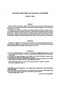
4. Results The results of the experiments are summarized in Figures 1{9. These gures show results on the dierent machines at T42, T85, and T170 resolution, expressed in terms of execution time for a ve-day forecast, execution rate in G op/sec, and M op/sec achieved per processor, all as a function of processor count. Results in these gures are for double precision. In addition, Figures 10 and 11 compare single- and double-precision performance on the SP2 and Paragon, respectively. Notice the use of a log scale in the X axis in all gures. In the gure keys, P represents Paragon, S represents SP2, and T represents T3D. On the Paragon, data were obtained on 128, 256, 512, and 1024 processors. On the SP2, data were obtained on 32, 64, and 128 processors. On the T3D, data were obtained on 64, 128, and 256 processors. Some problem sizes did not t on a small number of processors on the Paragon and hence are missing.

- 12 -

Time (seconds)

100 P L16 P L18 P L44 S L16 S L18 S L44 T L16 T L18 T L44 10

1 32

64

128 256 512 Number of Processors

1024

Figure 1: Execution times for 5-day forecast at T42 resolution (double precision).

Time (seconds)

1000 P L16 P L18 P L24 P L36 P L60 S L16 S L18 S L24 S L36 S L60 T L16 T L18 T L24 T L36 T L60

100

10 32

64

128 256 512 Number of Processors

1024

Figure 2: Execution times for 5-day forecast at T85 resolution (double precision).

- 13 -

Time (seconds)

10000 P L18 P L24 P L32 P L36 P L48 S L18 S L24 S L32 S L36 S L48 T L18 T L24 T L32 T L36 T L48

1000

100 32

64

128 256 512 Number of Processors

1024

Figure 3: Execution times for 5-day forecast at T170 resolution (double precision).

4 P L16 P L18 P L44 S L16 S L18 S L44 T L16 T L18 T L44

3.5

Gflop/second

3 2.5 2 1.5 1 0.5 0 32

64

128 256 512 Number of Processors

1024

Figure 4: Execution rate for 5-day forecast at T42 resolution (double precision).

- 14 -

7 P L16 P L18 P L24 P L36 P L60 S L16 S L18 S L24 S L36 S L60 T L16 T L18 T L24 T L36 T L60

6

Gflop/second

5 4 3 2 1 0 32

64

128 256 512 Number of Processors

1024

Figure 5: Execution rate for 5-day forecast at T85 resolution (double precision).

8 P L18 P L24 P L32 P L36 P L48 S L18 S L24 S L32 S L36 S L48 T L18 T L24 T L32 T L36 T L48

7

Gflop/second

6 5 4 3 2 1 0 32

64

128 256 512 Number of Processors

1024

Figure 6: Execution rate for 5-day forecast at T170 resolution (double precision).

- 15 -

30 P L16 P L18 P L44 S L16 S L18 S L44 T L16 T L18 T L44

Mflop/processor

25

20

15

10

5

0 32

64

128 256 512 Number of Proessors

1024

Figure 7: Processor performance for 5-day forecast at T42 resolution (double precision).

35 P L16 P L18 P L24 P L36 P L60 S L16 S L18 S L24 S L36 S L60 T L16 T L18 T L24 T L36 T L60

30

Mflop/processor

25 20 15 10 5 0 32

64

128 256 512 Number of Proessors

1024

Figure 8: Processor performance for 5-day forecast at T85 resolution (double precision).

- 16 -

40 P L18 P L24 P L32 P L36 P L48 S L18 S L24 S L32 S L36 S L48 T L18 T L24 T L32 T L36 T L48

35

Mflop/processor

30 25 20 15 10 5 0 32

64

128 256 512 Number of Proessors

1024

Figure 9: Processor performance for 5-day forecast at T170 resolution (double precision).

0.85 T42L16 T42L18 T42L44 T85L16 T85L18 T85L24 T85L36 T85L60 T170L18 T170L24 T170L32 T170L36 T170L48

Relative Time (Single / Double)

0.8

0.75

0.7

0.65

0.6

0.55 32

64

128 256 512 Number of Processors

1024

Figure 10: Ratio of double- to single-precision execution times for 5-day forecast on Paragon.

- 17 -

1.05 T42L16 T42L18 T42L44 T85L16 T85L18 T85L24 T85L36 T85L60 T170L18 T170L24 T170L32 T170L36 T170L48

Relative Time (Single / Double)

1

0.95

0.9

0.85

0.8

0.75 32

64

128 256 512 Number of Processors

1024

Figure 11: Ratio of double- to single-precision execution times for 5-day forecast on SP2.

5. Discussion We discuss a variety of issues relating to the performance results presented in the preceding section, including single node performance, parallel performance, the eect of arithmetic precision, and choice of algorithms. These issues are tightly interrelated.

5.1. Single-Node Performance Table 4 indicates a considerable variation in single-node performance across the three machines. While all have high \peak" uniprocessor performance ratings (75, 266, and 150 M op/sec for the Paragon, SP2, and T3D, respectively, at double precision), none achieves a large fraction of their peak performance on PSTSWM. This is due to a variety of factors, including instruction set, cache size, and memory architecture, which we shall not address here. (However, we note that in the T3D, the second-level cache normally used with the DEC Alpha chip is missing, thereby signi cantly reducing performance. The second-level cache should be restored in the next-generation machine.) A signi cant factor aecting single-node performance is coding style, which we discuss below.

- 18 -

5.2. Parallel Performance Figures 1{9 present a large amount of data from which one can derive many interesting conclusions about the performance of the spectral transform method on the Paragon, and SP2, and T3D. Unfortunately, the unequal machine sizes hinder direct comparisons of scalability. Larger SP2 and T3D systems were not available to us, and local memory size and execution time constraints on the systems that we used for these experiments did not allow us to make ve-day runs using smaller numbers of processors on the Paragon and the T3D. Looking rst at raw performance, as measured in G op/sec, we see that the Paragon achieves the highest total performance: over 7 G op/sec for problem T170/L32 on 1024 processors. Machine performance (in G op/sec) varies signi cantly with both horizontal and vertical resolution on all machines; this eect is particularly noticeable for larger numbers of processors. With respect to vertical resolution, performance is in uenced by three factors. First, a powerof-two number of levels avoids ineciencies due to load imbalances on a power-of-two number of processors. While this is to some extent an artifact of the fact that the number of processors and the horizontal grid dimensions are both powers of two in our experiments, it is a common situation, and similar issues will arise for other problem and machine size assumptions. Second, for small numbers of vertical levels and large numbers of processors, decomposing across the vertical dimension tends to introduce load imbalance, as there are fewer levels than processors. The optimization process generally avoids this, at the cost of choosing extreme processor grid aspect ratios or choosing a parallel algorithm that does not decompose the vertical dimension, both of which may increase communication costs. Third, a larger number of levels increases the granularity of the computation, generally improving per processor performance. However, for large numbers of vertical levels on moderate or small numbers of processors, the local computation may not t well into cache, resulting in a performance degradation. This latter eect explains the superlinear scaling evident on a few of the graphs. The SP2 achieves the highest performance on 128 processors, where it is between 30% and 100% faster than a 128 processor T3D, and between 150% and 300% faster than a 128 processor Paragon. The SP2 performs relatively worse at low resolutions, and the T3D relatively better. This eect is a result of the poorer communication performance of the SP2: computation costs scale faster than communication costs with resolution. Very approximately, it appears that the SP2 with half as many processors is slightly slower than the T3D, except at T42 resolution where it is signi cantly slower. The SP2 with one quarter as many processors is roughly comparable to the Paragon at all resolutions, and the T3D with half as many processors is roughly comparable to the Paragon at all resolutions. The average M op/sec achieved per processor provides a measure of scalability. (Perfect parallel scalability would be represented by a straight horizontal line.) From Figures 7{9, we see that all three machines scale reasonably well, particularly at higher resolution. The occasional anomalous increase in per-processor performance with increasing number of processors is due to improved cache utilization as a result of the smaller granularity, as mentioned above.

- 19 -

5.3. Precision The relative performance on the three machines is aected by the choice of arithmetic precision. At the current time, the T3D supports only double precision (64-bit) arithmetic in Fortran, while the Paragon and SP2 support both single and double precision. Arithmetic precision has a signi cant and complex in uence on machine performance, since it aects raw processor performance, cache performance, memory performance, and interprocessor communication performance. Table 4 gives single processor PSTSWM performance data for the Paragon and the SP2 at single and double precision. On the Paragon, double precision is signi cantly slower. On the SP2 processor, double precision is faster, although not by the same factor as some other applications. (For example, the LINPACK benchmark achieves 134 and 72 M op/sec at double and single precision, respectively.) This situation probably re ects reduced cache hit rates due to increased memory trac. As we shall see, the SP2 generally performs better at single precision when PSTSWM is executed on multiple processors, no doubt because of reduced communication costs. In comparing PSTSWM multiprocessor performance, we report in Figures 1{9 only doubleprecision results. This yields a fair comparison for large problem resolutions, where the increased accuracy of double precision may be needed. For smaller problem sizes, single precision is generally considered to be sucient, and hence the comparison is unfair to the Paragon and SP2 in these cases. Figures 10 and 11 show the impact of precision on performance on the Paragon and the SP2. The Paragon is between 20% and 40% slower at double precision. Dierences are larger at higher resolution, where compute time is a larger fraction of total execution time, and more data must be communicated. The SP2 is slightly faster in a few instances, and in most other cases around 10% slower (one case is almost 25% slower) at double precision. There seems to be little pattern in the SP2 results, suggesting that overall performance is a complex function of processor performance, cache performance, and communication costs. For example, we would normally expect highresolution problems to perform better than low-resolution problems at double precision, since computation costs are proportionally higher. However, this is not always the case, suggesting that PSTSWM is not achieving good cache performance. This problem could potentially be corrected by restructuring the code.

5.4. Algorithms In the rst part of this section, we discussed machine performance without reference to the algorithms being used on dierent problem size/machine type/machine size con gurations. Yet there is considerable variability in the performance of dierent algorithms (Foster and Worley 1994; Worley and Foster 1994), and average performance would have been considerably worse if we had restricted ourselves to a single algorithm. Factors that can aect performance include the choice of FFT algorithm, LT algorithm, aspect ratio, the protocols used for data transfer,

- 20 and memory requirements. For brevity, we just make a few comments regarding algorithms here; more details about relative performance are provided in (Foster and Worley 1994; Worley and Foster 1994). Examining Table 2, our rst observations are that no single algorithm is optimal across a range of problem sizes and machine sizes and that dierent algorithms are optimal on dierent machines. The algorithm combination that is asymptotically optimal for large problems and large numbers of processors is T/T, which uses transposes for both the FFT and LT. Yet this combination is optimal in only 53% of the con gurations on the Paragon, 33% on the SP2, and 5% on the T3D. Another promising algorithm is T/D, which uses a distributed algorithm for the LT. This is optimal in 26%, 58%, and 67% of con gurations on the Paragon, SP2, and T3D, respectively. Another algorithm that is optimal in a surprisingly large number of cases is FFT algorithm \D," the distributed FFT. This algorithm is known to be less ecient than the transpose from a communication point of view in almost all situations. Nevertheless, it can be faster than the transpose algorithm in the context of PSTSWM, particularly when the number of vertical levels is not a power of two. This is because the transpose FFT must decompose in the vertical dimension when performing FFTs, which can result in a considerable amount of load imbalance when the number of vertical levels is small. Hence, we see this algorithm used in combination with various LT algorithms in 60% of the L18 cases. Memory requirements also help determine the choice of optimal algorithm for large problem and/or small numbers of processors. Here, distributed algorithms have an advantage in that they require less work space than the transpose algorithms using the same logical aspect ratio, and the choice of optimal algorithm becomes one between distributed algorithms using optimal aspect ratios, and transpose or mixed transpose/distributed algorithms using suboptimal, but space saving, aspect ratios. To provide more quantitative information on the impact of algorithm selection on performance, we present in Table 5 some relevant statistics. For brevity, we present results for just three problem sizes: T42 L18, T85 L36, and T170 L32, representing three common problem sizes used in atmospheric modeling. Table 5 is concerned with both algorithm and aspect ratio selection: each statistic is the ratio of the execution time for some nonoptimal algorithm or aspect ratio to the optimal algorithm/aspect ratio combination identi ed by our tuning process. 1) Row CLASS measures sensitivity to algorithm choice. We determined the optimal parallel implementation and aspect ratio for each of the four algorithm classes T/T, T/D, D/T, and D/D, and present statistics for the slowest of the four classes. Hence, these results indicate how much can be gained by using the optimal algorithm. Note that, since all algorithm classes are optimal for some combination of problem size and number of processors, none can be discarded a priori. 2) Row ASPECT measures sensitivity to aspect ratio. We determined the optimal algorithm class for each problem size and number of processors, and present statistics for a square or nearly sqare processor grid (aspect ratio 1:1 or 2:1). Hence, these results indicate

- 21 -

Table 5: The Impact of Algorithm Selection on Performance (see text for details) P S T 128 256 512 32 64 128 64 128 256 T42L18 - CLASS 1.14 1.11 1.08 1.07 1.28 1.49 1.18 1.15 1.16 T42L18 - ASPECT 1.33 1.17 1.00 1.05 1.51 1.73 1.16 1.05 1.00 T42L18 - REF 1.39 1.25 1.10 1.73 1.75 2.08 1.20 1.43 1.36 T85L36 - CLASS 1.17 1.19 1.26 1.18 1.17 1.02 1.33 1.15 1.09 T85L36 - ASPECT 1.26 1.14 1.27 1.10 1.04 1.32 1.08 1.14 1.04 T85L36 - REF 1.30 1.18 1.30 1.78 1.46 1.49 1.15 1.21 1.14 T170L32 - CLASS - 1.10 1.20 1.63 1.40 1.40 1.07 1.12 1.11 T170L32 - ASPECT * 1.35 1.73 1.04 1.00 1.01 1.01 1.00 T170L32 - REF * 1.37 2.29 1.73 1.56 1.19 1.16 1.13 the utility of tuning with respect to aspect ratio. An asterisk indicates that the given algorithm cannot be run on such a processor grid, because of memory or algorithmic constraints. 3) Row REF measures the cost of standardizing on both algorithm and aspect ratio. The statistics are for a \reference" algorithm that uses transpose algorithms for both FFT and LT, a 1:1 or 2:1 aspect ratio, and a simple communication protocol that is supported on all message-passing systems that we have experience with. It is meant to represent what a reasonable choice would have been if we had forgone all tuning. The CLASS and ASPECT data show that even when considered in isolation, the choice of algorithm class and aspect ratio can have a signi cant impact on performance: degradations of 20{30% frequently result from nonoptimal choices. The REF data shows even greater divergences from optimal, which we should expect as algorithm class, aspect ratio, and communication parameters are all standardized and hence nonoptimal in most situations. The reference algorithm works well when the optimal algorithm is a transpose algorithm on a nearly square grid. However, in other cases it can be as much as 129% worse than the optimal algorithm. In general, the results emphasize the importance of performance tuning, particularly when performing performance comparisons of dierent machines. (The degree of degradation varies signi cantly between the dierent MPPs.) Notice that the optimal algorithm for a particular algorithm class varies across machines and that a reference algorithm for the T/D, D/T, and D/D classes would perform as badly, or worse, than the performance of the T/T reference algorithm. See (Worley and Foster 1994) for more details on the performance improvement possible from tuning within algorithm classes. These results lead us to conclude that parallel spectral transform codes should include run-time or compile-time tuning parameters, so that performance can be retained when moving between platforms or when hardware or software is upgraded. Our success with PSTSWM suggests

- 22 that with careful design, a large number of algorithmic options can be incorporated in a single code without greatly complicating its implementation. We suspect that similar techniques can usefully be applied in other models.

5.5. Price Performance We have not attempted to compare the price-performance (performance per unit of capital investment) of the dierent machines, because of the diculty of obtaining accurate price data and its dependence on nontechnical factors. However, this information must clearly be taken into account when interpreting the results of this study.

5.6. Coding Style We have attempted in this study to eliminate the eect of algorithm choices and communication protocols on performance. However, we have not addressed the related issue of coding style. PSTSWM was designed to emulate the coding style of PCCM2 (Drake et al. 1994), the message-passing parallel implementation of CCM2, and we believe that this design goal has been achieved. An advantage of this structure is that our results are directly applicable to PCCM2 and parallel implementations of similar models. A disadvantage is that achieved performance is not optimal. Many CCM2 data structures and algorithms have been selected to optimize performance on Cray-class vector multiprocessors. These same structures and algorithms are not necessarily ecient on the cache-based RISC microprocessors used in MPP systems. Certain computational kernels within PSTSWM (and PCCM2) have been restructured to run more eciently on RISC microprocessors. Nevertheless, it appears that cache data reuse remains low. For example, the T3D's hardware monitor indicates that the ratio of oating point operations to memory accesses is only 1.3. Very dierent coding structures would be required to improve this ratio. We are currently exploring such structures. The performance of PSTSWM can be improved by exploiting optimized FFT library routines and more aggressive code restructuring to allow, for example, the use of level 3 BLAS. We are hesitant to make code modi cations to PSTSWM that would be dicult to emulate in PCCM2, but one advantage of a code like PSTSWM is that it provides us with a testbed in which we can experiment with various optimization techniques before making changes in the production code.

6. Conclusions The experiments reported in this paper provide a number of valuable insights into the relative performance of dierent MPP computers and dierent spectral transform algorithms, and the techniques that should be used when constructing parallel climate models.

- 23 Our results indicate that massively parallel computers such as the Paragon, SP2, and T3D are indeed capable of multi-G op/sec performance, even on communication-intensive applications such as the spectral transform method. Ignoring issues of price performance, we nd that none of the parallel computers is consistently better than the others. The SP2 has the best uniprocessor performance, without which of course good parallel performance is dicult to achieve, and is also the fastest machine on 128 processors. On the other hand, the SP2 has poorer communication performance than the Paragon and T3D. The Paragon achieves the greatest peak performance (on 1024 processors). We also nd that many dierent aspects of algorithm and program design can have a signi cant impact on performance. In addition, optimal choices for parallel algorithm, communication protocols, and coding style vary signi cantly from machine to machine. Hence, performance tuning is important both when developing a spectral model for a single computer, and when developing a model intended to operate on several dierent computers. We believe that the solution to this problem is to design codes that allow tuning parameters to be set at run-time. This approach supports both (performance) portability and the empirical determination of optimal parameters.

Acknowledgments This research was supported by the Atmospheric and Climate Research Division of the Oce of Energy Research, U.S. Department of Energy, under Contracts W-31-109-Eng-38 and DEAC05-84OR21400. We are grateful to members of the CHAMMP Interagency Organization for Numerical Simulation, a collaboration involving Argonne National Laboratory, the National Center for Atmospheric Research, and Oak Ridge National Laboratory, for sharing codes and results; to Hubertus Franke of IBM for providing his MPI-F library on the SP2; to the SUNMOS development team for help in getting PSTSWM running under SUNMOS on the Intel Paragon; and to James Tuccillo of Cray Research for facilitating the Cray T3D experiments. This research was performed using the Intel Paragon system at Oak Ridge National Laboratory, the Intel Paragon system at Sandia National Laboratories, a Cray T3D at Cray Research, the IBM SP2 system at Argonne National Laboratory, and the IBM SP2 system at NASA-Ames Laboratory.

References Barros, S. 1994. Personal communication. Bourke, W. 1972. An ecient, one-level, primitive-equation spectral model, Mon. Wea. Rev.,

- 24 102, 687{701. Browning, G. L., J. J. Hack, and P. N. Swarztrauber, 1989. A comparison of three numerical methods for solving dierential equations on the sphere, Mon. Wea. Rev., 117, 1058{1075. Dent, D. 1990. The ECMWF model on the Cray Y-MP8, in The Dawn of Massively Parallel Processing in Meteorology, G.-R. Homan and D. K. Maretis, eds., Springer-Verlag, Berlin. Drake, J., I. T. Foster, J. Hack, J. Michalakes, B. Semeraro, B. Toonen, D. Williamson, and P. Worley, 1994. PCCM2: A GCM adapted for scalable parallel computers, in Proc. 5th Symp. on Global Change Studies, American Meteorological Society, pp. 91{98. Foster, I. T., W. Gropp, and R. Stevens, 1992. The parallel scalability of the spectral transform method, Mon. Wea. Rev., 120, 835{850. Foster, I. T., and B. Toonen 1994. Load-balancing algorithms for climate models, in Proc. Scalable High Performance Computing Conf., IEEE Computer Society, pp. 674{681. Foster, I. T., and P. H. Worley, 1993. Parallelizing the spectral transform method: A comparison of alternative parallel algorithms, in Parallel Processing for Scienti c Computing, R. F. Sincovec, D. E. Keyes, M. R. Leuze, L. R. Petzold, and D. A. Reed, eds., Society for Industrial and Applied Mathematics, Philadelphia, pp. 100{107. Foster, I. T., and P. H. Worley, 1994. Parallel algorithms for the spectral transform method, Tech. Report ORNL/TM-12507, Oak Ridge National Laboratory, Oak Ridge, Tenn., April (also available as a preprint from Argonne National Laboratory). Fox, G., R. Williams, and P. Messina, 1994. Parallel Computing Works!, Morgan Kaufman. Franke, H., P. Hochschild, P. Pattnaik, J.-P. Prost, and M. Snir, 1994. MPI-F: Current status and future directions, Proc. Scalable Parallel Libraries Conference, Mississippi State, October, IEEE Computer Society Press. Gartel, U., W. Joppich, and A. Schuller, 1993. Parallelizing the ECMWF's weather forecast program: The 2D case, Parallel Computing, 19, 1413{1426. Gropp, W., E. Lusk, and A. Skjellum, 1995. Using MPI: Portable Parallel Programming with the Message Passing Interface, The MIT Press. Hack, J. J., B. A. Boville, B. P. Briegleb, J. T. Kiehl, P. J. Rasch, and D. L. Williamson, 1992. Description of the NCAR Community Climate Model (CCM2), NCAR Tech. Note NCAR/ TN{382+STR, National Center for Atmospheric Research, Boulder, Colo.

- 25 Hack, J. J., and R. Jakob, 1992. Description of a global shallow water model based on the spectral transform method, NCAR Tech. Note NCAR/TN-343+STR, National Center for Atmospheric Research, Boulder, Colo., February. Kauranne, T., and S. Barros, 1993. Scalability estimates of parallel spectral atmospheric models, in Parallel Supercomputing in Atmospheric Science: Proceedings of the Fifth ECMWF Workshop on Use of Parallel Processors in Meteorology, G.-R. Homan and T. Kauranne, eds., World Scienti c Publishing Co. Pte. Ltd., Singapore, pp. 312{328. Loft, R. D., and R. K. Sato, 1993. Implementation of the NCAR CCM2 on the Connection Machine, in Parallel Supercomputing in Atmospheric Science: Proceedings of the Fifth ECMWF Workshop on Use of Parallel Processors in Meteorology, G.-R. Homan and T. Kauranne, eds., World Scienti c Publishing Co. Pte. Ltd., Singapore, pp. 371{393. Pelz, R. B., and W. F. Stern, 1993. A balanced parallel algorithm for spectral global climate models, in Parallel Processing for Scienti c Computing, R. F. Sincovec, D. E. Keyes, M. R. Leuze, L. R. Petzold, and D. A. Reed, eds., Society for Industrial and Applied Mathematics, Philadelphia, pp. 126{128. Walker, D. W., P. H. Worley, and J. B. Drake, 1992. Parallelizing the spectral transform method. Part II, Concurrency: Practice and Experience, 4, 509{531. Washington, W., and C. Parkinson, 1986. An Introduction to Three-Dimensional Climate Modeling, University Science Books, Mill Valley, Calif. Williamson, D. L., J. B. Drake, J. J. Hack, R. Jakob, and P. N. Swarztrauber, 1992. A standard test set for numerical approximations to the shallow water equations on the sphere, J. Computational Physics, 102, 211{224. Williamson, D. L., and P. J. Rasch, 1989. Two-dimensional semi-Lagrangian transport with shape-preserving interpolation, Mon. Wea. Rev., 117, 102{129. Worley, P. H., and J. B. Drake, 1992. Parallelizing the spectral transform method, Concurrency: Practice and Experience, 4, 269{291. Worley, P. H., and I. T. Foster, 1994. Parallel spectral transform shallow water model: A runtime-tunable parallel benchmark code, in Proc. Scalable High Performance Computing Conf., IEEE Computer Society Press, Los Alamitos, Calif., pp. 207{214.