Application of Reinforcement Learning for the Generation of an Assembly Plant Entry Control Policy E. Kehris Dept. of Business Administration Technological Educational Institute of Serres Serres, GREECE
[email protected]
Abstract The generation of an entry control policy for an assembly plant using a reinforcement learning agent is investigated. The assembly plan studied consists of ten workstations and produces three types of products. The objective of the entry control policy is to produce a given production mix within a planning horizon, while following a given production mix. Due to the large state space, a function approximator, based on a neural network, is used to model the long-term reward function. The schedules generated by the trained agent are compared to those produced by a deterministic heuristic control policy that has been developed for this assembly plant. Simulation results show that the reinforcement learning agent produces production plans that achieve better productivity than the heuristic controller under tight planning horizons, generating sub-optimal yet acceptable production mix balance.
1. Introduction Production scheduling deals with the allocation of the resources of a manufacturing system to a set of activities so as to optimize managerial objectives while satisfying system constraints. Typical managerial objectives include the minimization of make span, mean flow time, tardiness or the maximization of the resource utilization, while system constraints are related to the order in which the various processing activities are performed. Production scheduling problems usually belong to the NP-complete class of problems [1, 2]. Real-life scheduling problems are not amenable to analytical treatment and are studied mainly by developing specialized heuristics which often exploit individual characteristics of the manufacturing system and generate satisfactory but not optimal
D. Dranidis Computer Science Department CITY Liberal Studies Affiliated Institution of the University of Sheffield Thessaloniki, GREECE
[email protected]
schedules. More recently, machine-learning techniques have been employed in an attempt to address production scheduling. In this paper, we investigate the application of a reinforcement learning (RL) in production scheduling. Production scheduling is often treated [3, 4] as a two-level decision process: at the upper level the entry control policy (system loading) is decided, while at the lower level the job routing and job sequencing are determined. The entry control policy determines the time and the type of the part to be loaded into the system, usually taking into account general system requirements (e.g. the required production mix, the time horizon) and system’s state (e.g. work-in-progress, bottleneck machine status). Job routing, on the other hand, deals with the assignment of operations to the manufacturing system machines and is required in cases in which some of the machines of the manufacturing system have the capability of carrying out more than one processing operations. Job sequencing, finally, identifies the job to be processed in a specific machine by selecting the job from a nonempty set and it is required whenever a set of jobs are simultaneously requesting to be processed by the same machine. A practical and widely used approach to solving the job sequencing problem is the adoption of heuristic dispatching rules, such as FIFO or LIFO. This research investigates the application of a reinforcement learning approach in developing an upper-level controller that determines the entry control policy for a manufacturing system. To our knowledge no research has been reported to deal with this particular problem. The aim of the RL controller is to produce production schedules for the given manufacturing system which satisfy the demand while keeping a good balance of the production mix.
The structure of this paper is as follows: section 2 describes the reinforcement learning approach and its application to production scheduling, section 3 presents the manufacturing system which is used as a case study, the managerial objectives that should be met by the schedulers that feed the manufacturing system and a heuristic controller that has been used for loading the manufacturing system. The reinforcement learning agent developed for the specific manufacturing system is described in section 4, together with the results obtained when the RL agent is used to control the manufacturing system. A comparison of the RL agent to a heuristic controller is also presented in section 4. Section 5 concludes the paper by discussing the main finding of this research.
α t ∈ A (A is a finite set of actions) according to its current policy π : S → A . The action α t leads the system to its new state s t +1 and results an immediate reward rt +1 . RL algorithms usually employ stochastic action selection policies. A frequently used policy is the εgreedy policy: at each state the agent chooses with a probability 1-ε the action that returns the maximum expected long-term reward (a greedy action) and with a probability ε a random action (an explorative action). The estimated return is represented by the action value function Q : S × A → ℜ . A greedy action corresponds to the action associated with the maximum action value:
2. Reinforcement Learning
V ( st ) = max(Q( st ,α t )) . αt
RL algorithms approximate dynamic programming on an incremental basis. In contrast to dynamic programming, RL algorithms do not require a model of the dynamics of the system and can be used online in an operating environment. A reinforcement learning agent senses its environment, takes actions and receives rewards depending on the effect of its actions on the environment. The agent has no knowledge of the dynamics of the environment (it cannot predict the consequences of its actions). Rewards provide the necessary information to the agent to adapt its control policy. The aim of a reinforcement learning agent is to maximize the total reward received (simply called return) from the environment. For successfully applying a RL algorithm the system has to be represented as a stationary Markov Decision Process (MDP). Figure 1 illustrates the interaction of the RL agent with the system.
System
αt
rt +1
st
V : S → ℜ is called the state value function. V ( st ) is an estimation of the expected return when beginning from state st the agent follows a strictly greedy policy. In tasks in which there is a final state the expected return Rt starting from state st may be calculated as the sum of immediate rewards:
Rt = rr +1 + rt +2 + L + rT Tasks which have a final state are called episodic and the agent-system interaction from the initial to the final state is called an episode. To allow learning in non-episodic task (non-terminating tasks) a discount rate γ ( 0 ≤ γ ≤ 1 ) is introduced which discounts the present value of future rewards:
Rt = rr +1 + γrt + 2 + γ 2 rt +3 + L + γ n rt + n +1 + L To progressively improve the control policy of the RL agent when a near greedy policy is followed, the estimations of the expected return, as represented by the action values Q ( st ,α t ) , need to be updated during the agent-system interaction. One of the most popular RL algorithms is the Q-learning algorithm [5]. The update of the action values Q ( st ,α t ) with the Qlearning algorithm are:
Q ( st , α t ) ← Q ( st , α t ) + aδ t
RL agent Figure 1. The interaction of the RL agent with the simulation system.
where α parameter and
( 0 < α < 1 ) is a positive step-size
δ t = r t +1+γ max Q( st +1 , α ) − Q( st , α t ) α
= r t +1+γV ( st +1 ) − Q ( st , α t ) If s t ∈ S (S is a set of states) is the state of the system at time t then the RL agent decides the action
δ t is the “error” of the estimation of the return. The target value of Q ( st ,α t ) is equal to the immediate received reward
rt +1 plus the discounted estimated
state value V ( st +1 ) of the next state. Learning is based on temporally successive estimates of Q; this sort of learning is typical in Temporal Difference (TD) reinforcement learning algorithms. In the case of Q-learning the agent is able to learn the estimates of the optimal policy independently of the policy being followed (the agent does not need to take the best action at the next state). Therefore Q-learning is considered an off-policy control algorithm. Another algorithm that can be used for the update of the action value function Q is the Sarsa algorithm [6]. In Sarsa the error δ t is:
δ t = r t +1+γQ ( st +1 , α t +1 ) − Q ( st , α t ) In Sarsa, the target value of Q ( st ,α t ) is equal to the immediate received reward rt +1 plus the discounted estimated action value Q ( st +1 , α t +1 ) of the next action taken at the next state. Sarsa, in contrast to Q-learning, is an on-policy control algorithm. The agent learns the estimates of the policy being followed. Due to the near-greedy policy, better estimations of the followed policy, progressively result in better control policies. Exploration is necessary for the agent to discover better states and actions in order to improve its policy. To improve the efficiency of RL algorithms, they can be combined with eligibility traces. Eligibility traces keep track of the states visited and the actions taken so far and thus allow multiple updates of the action value function Q. The value of using eligibility traces increases significantly in tasks which have long episodes and delayed rewards. The eligibility trace for state s and action α at time t is denoted e( st , at ) . Each time an action is taken at some state, the corresponding eligibility trace is increased by 1. At the same time, all eligibility traces are decayed by γλ, where γ is the discount rate and λ is the trace-decay parameter. The update of the action value function is performed for all states-action pairs s and a:
Q ( s, a ) ← Q ( s, a) + αδ t et ( s, a ) Only the visited state-action pairs which are tracked by the eligibility traces are actually updated. Both Qlearning and Sarsa can be combined with eligibility traces and are called Q(λ) and Sarsa(λ) respectively. In the case of Q(λ), however, all eligibility traces must be set to zero after an exploratory action is taken.
For problems in which the state space is small a table can be used for storing the action value function Q. In real world problems, however, the state space is too large or even continuous, and the Q function cannot be represented in a tabular way. In these cases function approximation techniques are employed to approximate the Q function. Function approximation can be achieved by representing Q as a function of a parameterized vector. For example, if an artificial neural network is used, then the Q a function (where
Q a ( st ) = Q( st , a) )
can
be
represented
as
a
parameterized function of the state as input and the r connection weights vector wt as the parameter vector, and a gradient descent technique (such as r backpropagation [7]) may be used to adjust wt . A separate output unit, representing the value of Q a ( st ) , has to be used for each action α ∈ A . Since states are indirectly represented by the weights vector, eligibility r traces are represented as a vector et (one trace for each
r
component of wt ). The updates of the weights vector are:
r r r wt ← wt + αδ t et
where
r r et ← γλet + ∇ wrt Q ( st , at )
δ t is the error in the estimation of Q, as it was described above. The derivative vector ∇ wr Q ( st , at ) t
r
is the gradient of Q ( st , at ) with respect to wt . Intuitively, the weights which contribute more to the calculation of the Q value have larger eligibility traces. The pseudocode for Sarsa(λ) with a backpropagation network as the function Q approximator is given below: initialize weights vector set eligibilities vector e to zero set s as the initial state Q = ΝΝw(s) (forward propagate) a = arg maxa Q(a) with probability ε: a = random action
repeat decay all eligibilities by γλ update eligibilities for action a (back propagate) take action a, observe reward r, and next state s δ = r - Q(a)
Q = ΝΝw(s) (forward propagate) a = arg maxa Q(a) with probability ε: a = random action
if s is not terminal δ = δ + γQ(a) update weights vector w based on δ and e Q = ΝΝw(s) until s is terminal
(forward propagate)
2.1. Related work Probably the most impressive application of Reinforcement Learning is the TD-Gammon system [8], which achieved a master level in backgammon by applying the TD(λ) reinforcement learning algorithm (Temporal Difference algorithm [9]). In TD-Gammon a neural network receives the full representation of the board and approximates the value function. Successful applications of RL algorithms to control problems have been reported. Crites and Barto [10], for example, employed RL algorithms for elevator dispatching. A team of RL agents using neural networks were trained to improve the performance of multiple elevator systems. Zhang and Dietterich [11] applied a RL method that learns to incrementally improve a repairbased job-shop scheduler for the payloads placed in the cargo bay of the NASA space shuttle. Their objective was to schedule a set of tasks without violating any resource constraints while minimizing the total duration. They use the TD(λ) algorithm (the same algorithm used in TD-Gammon) to learn an evaluation function over states of scheduling. A number of researchers have reported on employing reinforcement learning to address various problems related to manufacturing. Mahadevan et al. [12], for example, introduced a model-free algorithm for average-reward RL (called SMART). They apply the algorithm in controlling a production-inventory system with multiple product types. In their system, there was a single machine capable of producing multiple types of products with multiple buffers for storing each of the different products. Whenever a job is finished, the machine may either undergo maintenance or start another job. The RL agent has to decide between these two actions in order to avoid costly repairs. Mahadevan and Theocharous [13] applied SMART to a 3-machine transfer line producing a single product type. Their goal was to maximize the throughput of the transfer line while minimizing its work-in-process inventory and failures. They compared
the policy from SMART to the kanban heuristic. Their results showed that the policy learned by SMART requires fewer items in inventory and results in fewer failures than with the Kanban heuristic. A number of researchers deal with the jobsequencing problem. Liu and Dong [14] used the Qlearning algorithm to train a neural network to select the most appropriate dispatching rules. Their results showed that the dispatching rules that are known to provide good results have higher probabilities of being selected by their trained neural network than the least desirable rules. In a similar approach, Wan and Usher [15] employed the Q-learning algorithm to the dispatching rule selection problem for a single machine. Their results showed that an agent trained with the Q-learning algorithm is able to identify the best rules for different system objectives. Aydin and Öztemel [16] report similar results using the Q-III reinforcement learning algorithm. System scheduling (i.e. upper-level scheduling) bears some similarities to lower level scheduling since in both cases the objective is to determine the next job to be processed. However, the aim of system schedulers is much more complicated for a number of reasons: Firstly, system schedulers should consider the possibility of not loading any job into the system: given a production mix that has to be satisfied within a time horizon, there may be time instances at which the system scheduler decides not to load any part into the system, e.g. due to excessive work in progress. This option is not considered at machine-level job scheduling: whenever a set of jobs are simultaneously requesting to be processed by an available machine, one of them is always loaded to the machine. Furthermore, the machine-level schedulers reported in the literature, are presented with a small number of heuristic dispatching rules and attempt to develop a new policy by applying the most appropriate dispatching rule taking into account the system status. At any decision point, the machine-level dispatcher has to select one of the available dispatching rules. In the problem we consider, however, the set of available actions is not constant: at some points of time, some of the actions considered by the system scheduler may not be feasible e.g. because the machine required to process a part type is busy and its local buffer is full. In addition, machine-level controllers reported in the literature aim to optimize the performance of a single machine. The system-level controller we consider in our work aims at optimizing the performance of the whole manufacturing system which consists of a number of machines. As a result, our system-level controller needs to generate a control
policy by considering the overall system status, while the actions taken may at some points deteriorate the performance of some machines in favour of improving the overall system performance. The systems reported in the literature consider a single machine, which process parts from an input buffer. The machine performs one operation at a time. As a result, at any point of time, the action to be taken is the selection of one part out of the input buffer. The next time at which a decision is required is when the machine completes the operation of the selected part. Similarly, in the manufacturing system we consider, the machines operate on parts selected from their input buffers and process them. In contrast to the systems reported in the literature, however, in our system, while the machine is carrying out an operation, (i.e. without any obvious state change) the scheduler may still decide whether to add another part in the machine's input buffer. This characteristic renders the system status more "continuous". Finally, the manufacturing system we study is initially empty. The existence of many machines and the necessary set up operations result to a long transient period during which the RL agent takes actions without any obvious immediate effect. The effect of the actions taken by the RL agent become obvious at a later stage, when the parts start to be produced. This long transient period may have an affect on the behaviour of the RL agent. These features place additional difficulties on the application of RL to a system-level loading scheduler in comparison to a machine-level scheduler. The manufacturing system used to study the applicability of the RL approach on developing a system-level scheduler is described next.
3. The manufacturing system The manufacturing system studied in this paper is a simplification of an existing assembly plant. In its simplified version, the assembly plant we consider consists of ten different workstations and produces three types of printed circuit boards (PCBs) referred to as Type A, B and C. The manufacturing system consists of ten workstations shown in Table 1. The workstations do not suffer from breakdowns but some of them require set up. More explicitly, the automatic surface mounting (workstation 2) and the Integrated Circuit testing machines (workstation 10) require a set up operation when a change in the type of board is encountered. Table 1 shows the set-up times for each machine of the workstation.
Parts waiting to be processed by the workstations are temporarily stored at workstation’s local input buffer which is of capacity of two. The dispatching rule used to select the next part to be processed from an input buffer is the FIFO rule.
Table 1: The workstations manufacturing system. Work station Id 1 2 3 4 5 6 7 8 9 10
Workstation Name
of
the
Setup time
Solder paste painting Surface Mounting Reflow soldering SMD vision control Assembly Assembly Wave soldering Final assembly Vision control Integ. circuit test
12 sec
24 sec
Table 2: The routing of the part types. Board Type A B C
Routing (workstation id) 1 1 1
2 2 2
3 3 3
4 4 4
5 5 6
7 7 7
9 8 8
10 10 9
10
The routings of the three types are given in Table 2 in terms of the sequence of the workstations they have to visit to complete their assembly. Each of operation required by the part types is carried out by one machine only and thus job routing is not required. The duration of the corresponding operations are given in Table 3. It is evident from the duration of the processes that the setup operation is a time-consuming activity.
Table 3: Processing Times (in sec). Board Type A B C
1 3 3 3
2 3 3 5
3 11 11 11
Workstation id 4 5 6 7 7 11 -- 19 13 20 -- 19 15 -- 11 19
8 -14 4
9 3 4 4
10 2 1 6
A typical production mix for the manufacturing system, which must be satisfied within a time horizon that ranges between 1100 and 1300 time units, is shown in Table 4.
• Table 4: A typical production mix.
Data Collection - Defines the user-defined parts of the system for which data collection is necessary.
•
Type A B C
Quantity 20 5 30
3.1. The Simulation Program A simulation model that mimics the manufacturing system described earlier was built using the FMSLIB simulation library [17] which is a generic software library written in C that facilitates the simulation of manufacturing systems and their real time control strategies. FMSLIB employs the three-phase approach [18] and provides facilities for modelling the physical structure, the part flow and the system and workstation loading policy of a family of FMSs. FMSLIB currently supports the following simulation entities: • parts of different types • machines • workstations (a group of machines) • limited capacity buffers • non-accumulating conveyors FMSLIB advocates the separate development of the conceptually different views of the simulated system. This approach facilitates the modular program development, program readability and maintainability and the evaluation of different strategies (system-level control policy, dispatching control, etc) on the same system. A simulation program based on FMSLIB is comprised of the following modules: • Physical Structure (Equipment) - Contains the descriptions of the machine, conveyor, buffer and workstations that make up the simulated system
•
•
•
Operational Logic - Contains the descriptions of the feeding policies for the machine, workstation and conveyors of the simulated system i.e. determines the input buffer policy for each machine. Input Data - Provides system-related static data like the demand and the machine processing times Part path - Describes the part flow through the system. This module explicitly describes the equipment required by each part type, at each stage of its manufacturing process.
Control Strategy - Determines the system-level scheduling policy to be implemented for the control of the system; i.e. it determines which part type will be introduced in the system and when. In this paper, the control strategy is implemented by the neural network which is trained using the RL agent. The separation of the different views of the simulated system advocated by FMSLIB greatly facilitated the incorporation of the software that implements the RL agent (written in C++) with the simulation code.
3.2. Heuristic controller The manufacturing system described earlier is fed by a heuristic controller which determines the time and the type of the part to be introduced into the system [19]. An important managerial objective of the scheduling policy that must be satisfied by any control policy for this system is to ensure timely demand satisfaction and balanced production rate of the required types. This means that ideally the production rates of the three types must be constant during production. The balanced production requirement is necessary because the assembly plant feeds successive production stages. In this section we provide a short description of the heuristic algorithm without getting into details (e.g. the treatment of machine break downs) which are of no interest for this work. The heuristic algorithm employed for the system loading policy consists of two steps: (a) the part types that are candidate for loading into the system are identified and (b) the type of the part to be loaded in the system is decided. The type of the part to be loaded into the system is the one having the maximum backlog of the cumulative entrance from a boosted desired, where the backlog for type i is calculated by the expression: bi (t ) = d i (t + Ti ) − ei (t ) if ei (t ) < Pi otherwise
bi (t ) = −ei (t ) where • t is the current time, Pi is the production demand; • d i = Pi T is the demand rate (T is the planning horizon) for product type i
35
Parts produced
30
15 10
1071
957
1015
901
820
764
706
650
592
541
455
451
0
389
5
338
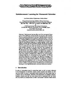
The behavior of the heuristic controller under the range of typical planning horizons and for the typical production requirements shown in Table 4 is discussed next. Simulation results show that the heuristic controller achieves very stable production balances under a wide range of planning horizons. When the planning horizon is sufficiently long, the heuristic controller achieves a nearly ideal production mix. For example, when the planning horizon is set to 1300 time units the heuristic controller produces all the required parts of Table 4 following closely the ideal production rates. This is shown in Figure 2 which displays the actual production achieved by the heuristic algorithm (stepwise lines) together with the ideal production rates (straight lines). However, when the planning horizon is tight, the heuristic algorithm produces an extremely balanced production mix at the cost of a significantly lower total production. For example when the planning horizon is set to 1100 time units, the total production for types A, B and C is 16, 4 and 24 parts respectively – instead of the 20, 5 and 30 parts required. The production rates achieved by the heuristic controller for this case are extremely balanced throughout the planning horizon as it is shown in Figure 3.
20
280
The part types that are candidates for loading into the system are those having positive backlogs bi (t ) .
25
224
for product type i.
30
59
•
product type i; and ei (t ) the number of entered parts at time t
35
143
Ti is the estimated processing time for for Parts produced
•
Tim e Type C
Type B
Type A
Figure 3. The production achieved by the heuristic controller for a tight production horizon.
3.3. Scheduling policy objectives The aim of this research is to develop a RL-based controller which under tight planning horizons achieves better productivity than the heuristic controller generating sub-optimal – but still acceptable – production rates. The system scheduling policy we consider is responsible for deciding the time instances at which a part will be input in the manufacturing plant as well as the part type. The objective of the scheduling policy is to ensure timely demand satisfaction and as balanced production rate of the required types as possible. This means that ideally the production rates of the three types must be constant during production. The simulation program that has been developed for modeling the dynamics of the manufacturing system is supervised by an RL agent that determines the loading policy of the simulated plant. The details of the RL agent developed are discussed in the next section.
25
4. The Reinforcement Learning agent
20
15
10
1302
1244
1162
1104
965
1023
927
869
788
706
672
591
509
423
393
312
254
59
0
168
5
Tim e Type C
Type B
Type A
Figure 2. The production achieved by the heuristic controller for a sufficiently long planning horizon.
The definition of a reinforcement learning agent consists of: • a state representation, • a reward function, • an action selection control policy, and • a learning algorithm for estimating the state (or action) values. All these decisions are very important for the success of an RL agent. The above elements of the RL agent are described in the following sections.
4.1 State representation One of the most important decisions when designing an RL agent is the representation of the state. In the system described in this paper this is one of the major concerns since a complete representation is not possible due to the complexity of the problem. Therefore we choose to include the following information in the state representation: • state of machines. Each machine may be found in one of four distinct states: idle, working, setup or blocked.
•
state of input buffers. Buffers are of limited capacity.
• backlogs for each type of production parts. Due to the large state space a neural network is used for approximating the value function. Specifically the neural network input layer consists of the following units: • 4 input units are used for each one of the machines. Each input unit corresponds to one of the possible states (idle, working, setup or blocked) •
2 units are used for each buffer. One unit for the level of the buffer and a second one which turns on when the buffer is full.
•
10 one-dimensional Radial Basis Function Units are used for each production type backlog. Totally, there are 82 inputs for the input state representation. The backpropagation learning algorithm is used for updating the weights of the network.
4.2. The reward function The implicit mapping of the reward functions to scheduling policies has to be a monotonic function: higher rewards should correspond to better scheduling policies. Taking into consideration the scheduling policy objectives mentioned in a previous section, the reward is calculated with the following formula: M
r = − wbal
max p (τ ) − d τ ∑ τ =1
i
i
M
i
− wtim
M −T T
The formula consists of two scaled terms. The first term of the formula evaluates the balance of the production. At each time τ, the distance of the actual
production from the ideal production pi (τ ) − diτ is calculated for each product and the maximum absolute distance is summed for the whole duration of the production task. The result is divided by M, the total production time (make span) for the specific episode. Note that τ is used for simulation time to distinguish from decision epoch (times at which the RL agent takes decisions), which is denoted as t. The second term of the formula evaluates the timeliness of the production. T is the planning horizon, i.e. the required production should be accomplished within this time. In the ideal case M should be equal to T. So, the RL agent is punished with the sum of the maximum distance between the desired and actual amount of production and the distance between the total production time and the planning horizon. In the experiments conducted we have chosen the values wbal = 2 and wtim = 1 for the parameters. The reward is negative and its values generally range in the interval [-1,0). Simulation steps do not coincide with decision epochs of the RL agent, since during the simulations, there are states in which there is only one possible action (for example, when the input buffer is full the only possible action is “do nothing”). At these states the simulation proceeds without consulting the RL controller. However, rewards are still calculated at each simulation step and accumulated until the next decision epoch. The total reward accumulated and calculated as in the formula above is returned to the agent at the end of the episode.
4.3. Actions The RL agent has to decide between four actions: entering a part of type A, B or C or doing nothing. The decision is based on the output of the neural network, which is trained during the simulation. The activation function for the 4 output units is a sigmoid function translated by -1 to fit in the reward region.
4.4. RL learning algorithm The RL agent developed employes the Sarsa(λ) algorithm. This decision was justified by a specific characteristic of the particular manufacturing system. As explained earlier, some actions may be infeasible at some time instances of an episode. For example, if the entry machine is busy and its input buffer is full, no part may be added to the system. In RL algorithms, the updates of the current state-action value estimations are based on the estimated values of the next state.
Sarsa(λ), which is an on-policy algorithm, uses for the update the value of the next action followed, whereas Q(λ) uses the value of the best next action. If some actions are not possible at the next state (fact which is not known to the agent before visiting that state), then Q(λ) might wrongly update its estimates by using the value of an infeasible action. Sarsa, on the other hand, takes into account the action selection and therefore is more suitable to this task.
4.5. RL agent parameter setting The task of controlling the manufacturing system is an episodic task. Each simulation ends when all required products have been produced. Therefore, the discount factor γ is set equal to 1 (rewards are not discounted). Episodes are quite long (more than 1000 time steps) and the reward is provided to the agent once at the end of the long episode. Therefore, a large trace decay parameter λ was preferred (0.995), so that the reward can be propagated (through the eligibility traces) towards the actions taken at the beginning of the episode. Past traces decay with a factor λt where t is the number of time steps. Figure 4 illustrates the value of λt for different λ and time steps. Note that for λ=0.995 the decay trace falls below the value of 0.005 after about 1000 time steps. (Correspondingly: λ=0.90, 50 time steps; λ=0.95, 100 actions; λ=0.99, 500 actions). 1 0.9 0.95 0.99 0.995
0.1
0.01
0
100
200
300
400
500
600
700
800
900
1000 1100 1200
t
Figure 4: λ for different values of λ in logarithmic scale. Training the agent with randomly chosen weights for 40,000 episodes showed that a large value of λ (0.995) combined with relatively high alpha value (α=0.2) produces the best results. The action selection technique used is the ε-greedy policy with ε equal to 0.1 (10% of the decisions are random) to allow high exploration. The value of ε is decaying after each episode.
4.6 RL agent training The RL agent was trained to produce the typical production mix under a tight planning horizon (1100 time units). The total production time and the rewards explored by the RL agent during its training are shown in Figure 5. For testing purposes, the behavior of the agent during its training was observed by requesting it to periodically generate system loading schedules based on the knowledge it has gathered up to that point. Thus, every 100 episodes, the RL agent is used to control the manufacturing system for one testing episode. During the testing episode, the upper level scheduling policy of the manufacturing system is determined by the RL agent. The parameters ε and α are set to zero during the testing episodes to disable learning and random actions. The behavior of the RL based controller during the testing episodes is shown in Figure 6. In order to evaluate the balance of the production, we display the policy generated by the agent in a representative testing episode having a total production time of 1150 and reward -0.4 (Figure 7). The ideal cumulative productions (shown in the Figure 7 as three straight lines, one for each part type) may be compared with the production generated by the RL algorithm which (shown in the figure as three stepwise functions).
1400
1400 Make-span Moving Average
Make-span Moving Average
1350
1300
1300
1250
1250 TIME
TIME
1350
1200
1200
1150
1150
1100
1100
1050
1050
1000
1000 0
5000
10000 15000 20000 25000 30000 35000 40000 45000
0
5000
10000 15000 20000 25000 30000 35000 40000 45000
Episodes
Episodes
(a)
(a)
0
0 TIME-reward
-0.2
-0.2
-0.4
-0.4
Reward
Reward
TIME-reward
-0.6
-0.6
-0.8
-0.8
-1 1000
1100
1200
1300
1400
-1 1000
1500
1100
1200
Episodes
1300
(b)
1500
(b)
0
0
Episode reward Moving Average
Episode reward Moving Average
-0.2
-0.2
-0.4
-0.4
Reward
Reward
1400
Episodes
-0.6
-0.6
-0.8
-0.8
-1
-1
0
5000
10000
15000
20000
25000
30000
35000
40000
45000
Episodes
0
5000
10000
15000
20000
25000
30000
35000
40000
Episodes
(c)
(c)
Figure 5 : The behavior of the RL agent during training: (a) The total production time (b) The combination of reward – total production time (c) The reward achieved at each training episode.
Figure 6. The behavior of the RL agent during testing: (a) The total production time (b) The combination of reward – total production make span (c) The reward achieved at each testing episode.
45000
horizon (table 5, Figure 9). Considering the achieved reward values, the RL agent supersedes the heuristic controller for planning horizons 1100 and 1150 while for longer planning horizons, the heuristic controller is able to produce much better results (Figure 8).
Table 5. Average rewards and total production times for the heuristic controller and the RL Agent.
REWARD
AVERAGE MAKESPAN
AVERAGE REWARD
35
RL AGENT
MAKESPAN
HEURISTIC CONTROLLER PLANNING HORIZON
It can be observed (Figure 7) that the RL agent produces a schedule that is sub-optimal in the sense that it does not achieve the ideal production for part types A and C. However, the production schedule generated for the part type A is consistently higher than the ideal production, while the production for part type C is consistently lower than its corresponding ideal production. The deviation of the actual productivity from the ideal one that is noticed in the schedule generated by the RL agent is compensated by a considerable productivity: for a time horizon equal to 1100 time units, 19 parts of type A, 4 parts of type B and 19 parts of C are produced – instead of the 20, 5 and 30 parts required. This production is the 95% of the required. It is reminded that the heuristic controller for the same planning horizon produced 80% of the required parts (16 parts of type A, 4 parts of type B and 24 part of type C). In general, the RL agent produced a schedule which has a total production time close to the planning horizon while not sacrificing the requirement for an acceptable balance.
1100
1374
-0,59
1150
-0,4
1150
1398
-0,54
1163
-0,45
1200
1398
-0,44
1210
-0,47
1300
1302
-0,16
1290
-0,39
30
25
0 -0,1
20
Reward
-0,2 15
10
-0,3 -0,4 -0,5 -0,6
5
-0,7 1100
Type C
Type B
1150
98 2 10 67 10 97 11 55
95 2
86 6
80 8
75 5
67 3
58 9
55 9
50 6
45 3
39 5
30 5
27 5
19 3
79
13 6
0
Type A
Figure 7. Actual and ideal cumulative production achieved by the RL agent.
1200
1300
Planning horizon Heuristic Controller
RL Agent
Figure 8: The rewards achieved by the heuristic controller and the RL agent for different values of the planning horizon.
4.7. Comparison of the RL scheduler to the 300
In this section the performance of the RL scheduler is compared to that of a heuristic controller for a range of planning horizons. The average reward achieved (after training) for each time horizon shown in Table 5. It is observed that for planning horizons shorter than 1300 time steps the heuristic controller fails to respect the planning horizon in favor of a completely balanced production mix. On the other hand, the RL agent achieves schedules considerably closer to the planning
Difference of total production time from planning horizon
heuristic controller
250 200 150 100 50 0 -50
1100
1150
1200
1300
Planning horizon Heuristic controller
RL agent
References Figure 9: The distance of the total production time from the planning horizon for the Heuristic controller and the RL agent for different values of the planning horizon.
5. Conclusions RL is an approach that allows an autonomous agent to learn through interaction with its environment to select the proper actions in order to achieve its goal. The approach has been adopted with success in various fields and more recently it has been employed to address production scheduling problems related to the machine-level control of a manufacturing system. In this work we employ RL in order to develop a system level controller which determines the time and the type that a product must be introduced into the manufacturing system. The aim of the controller is to load product parts into the manufacturing system in such a way, that the production is accomplished within a time horizon, while the part types produced follow an ideal production rate. This is a demanding task and although it bears some similarities with research reported in the literature, the particular problem has not been addressed. Due to the large state space, the value function required by the RL agent is approximated by a neural network. Experimental results show that the RL agent learns to produce the required production mix within the given time horizon while consistently approaching the ideal production rates. Furthermore, simulation results show that under strict planning horizons the RL agent outperforms, in terms of productivity, a heuristic controller that has been used to control the manufacturing system. In such cases, the heuristic controller produces a very close to ideal balance production mix but fails to satisfy the production requirement. On the contrary, the RL agent is able to increase system productivity without sacrificing production balance. This may have important practical implications in cases where small deviations from the ideal production rates are acceptable if combined with considerable gains in productivity.
Acknowledgment This Project is co-funded by the European Social Fund and National Resources - (EPEAEK-II) ARHIMIDES
[1] T. E Morton,. and D. W Pentico,. Heuristic Scheduling Systems With Applications to Production Systems and Project Management, J. Wiley, 1993. [2] M. Pinedo, Scheduling Theory, Algorithms, and Systems, Prentice Hall, 1995. [3] R. Akella , YF Choong, SB Gershwin, Performance of hierarchical production scheduling policy, IEEE Trans. Components Hybrids Manufacturing Technology, Vol 7, No. 3, 1984, pp. 225-240. [4] R. Graves, Hierarchical scheduling approach in flexible assembly systems, Proceedings of the 1987 IEEE Conference on Robotics and Automation, Raleigh, NC, Vol. 1, 1987, pp. 118-123. [5] C.J. Watkins, P. Dayan. Q-learning. Machine Learning, 8, 1992, pp. 279-292.
[6] R. S. Sutton, Generalization in reinforcement learning: Successful examples using sparse coarse coding, in Touretzky, D. S., Mozer, M. C., and Hasselmo, M. E., editors, Advances in Neural Information Processing Systems: Proceedings of the 1995 Conference, Cambridge, MA. MIT Press, 1996, pages 1038-1044. [7] D.E. Rumelhart, G.E. Hinton., and R.J. Williams, Learning internal representations by error propagation, in Rumelhart, D. E. and McClelland, J. L., editors, Parallel Distributed Processing: Explorations in the Microstructure of Cognition, vol.1: Foundations. Bradford Books/MIT Press, Cambridge, MA., 1986 [8] G. Tesauro, TD-Gammon, a Self-Teaching Backgammon Program, Achieves Master-Level Play, Neural Computation 6, 1994, pp. 215-219. [9] RS Sutton, Learning to predict by the methods of temporal differences, Machine Learning, 3, 1988, pp. 9-44. [10] R. Crites, A. Barto, Improving Elevator Performance Using Reinforcement Learning. Touretzky DS, Mozer MC, Hasselmo ME, eitors, Advances in Neural Information Processing Systems 8, MIT Press, 1996. [11] Dietterich, Zhang. A reinforcement-learning approach to job-shop scheduling. Proceedings of the 14th International Joint Conference on Artificial Intelligence, 1995. [12] S. Mahadevan, N Marchalleck, TK Das, A Gosavi, Selfimproving factory simulation using continuous-time averagereward reinforcement learning, Proceedings of the 13th International Conference on Machine Learning, 1996, pp. 202-210. [13] S. Mahadevan, and G. Theocharous, G. Optimizing Production Manufacturing using Reinforcement Learning.
The 11th International FLAIRS Conference, AAAI Press, 372-377, 1988. [14] H. Liu, and J. Dong, Dispatching Rule Selection Using Artificial Neural Networks for Dynamic Planning and Scheduling. Journal of Intelligent Manufacturing, 7, 3, 1996 pp.243-150. [15] Y.C. Wang, J.M. Usher, Application of reinforcement learning for agent-based production scheduling, Engineering Applications of Artificial Intelligence, 18, (2005), 73-78) [16] M. Emin Aydin a, Ercan Öztemel Dynamic job-shop scheduling using reinforcement learning agents, Robotics and Autonomous Systems 33 (2000) 169–178.
[17] E. Kehris, Z. Doulgeri. An FMS simulation development environment for real time control strategies. XVI European Conference of Operational Research, Brussels, 1998. [18] K. Tocher, The Art of Simulation, Van Nostrand Company, Princeton NJ, 1963. [19] Z. Doulgeri, E. Kehris, Effect of Workstation Loading on the Objective of the System’s Entry Policy in FMS, Integrated Manufacturing Systems, Vol 14, No. 3, 2003, p. 293 – 304.