Reinforcement Learning for Scheduling of Maintenance

Reinforcement Learning for Scheduling of Maintenance Michael Knowles, David Baglee1 and Stefan Wermter2

Abstract Improving maintenance scheduling has become an area of crucial importance in recent years. Condition-based maintenance (CBM) has started to move away from scheduled maintenance by providing an indication of the likelihood of failure. Improving the timing of maintenance based on this information to maintain high reliability without resorting to over-maintenance remains, however, a problem. In this paper we propose Reinforcement Learning (RL), to improve long term reward for a multistage decision based on feedback given either during or at the end of a sequence of actions, as a potential solution to this problem. Several indicative scenarios are presented and simulated experiments illustrate the performance of RL in this application.

1 Introduction Condition-based maintenance (CBM) is an area which has received substantial attention in recent years. Prior to the advent of CBM, maintenance was either reactive, repairing faults as they occurred which led to downtime and the potential for extended damage due to failed or failing parts, or planned preventative maintenance which sought to prevent failures by performing maintenance on a pre-planned fixed schedule, where the reliability and efficiency of this approach depended on the appropriateness of the schedule [1,2]. CBM involves performing some measurement of the condition of equipment so as to infer the maintenance needs. Condition data is generally compiled from sensors recording various aspects of the equipment’s condition, including vibration measurements, temperature, fluid pressure and lubricant condition. Typically a series of thresholds are defined which trigger an intervention when the measurements go above these thresholds [3, 4]. Furthermore, several levels of 1

Institute for Automotive and Manufacturing Advanced Practice (AMAP), University of Sunderland, Colima Avenue, Sunderland, SR5 3XB, UK

2

Knowledge Technology Group, Department of Informatics, University of Hamburg, Vogt Koelln Str. 30, 22527 Hamburg, Germany

2

M.J. Knowles, D. Baglee and S. Wermter

alert are set depending on the level of seriousness of the fault. To fully exploit condition measurements, it is, however, necessary to be able to predict the precise implications of a given action under a particular set of condition measurements. This can be achieved using combinational limits which trigger alerts when several thresholds are passed but these must be set up either empirically or through detailed analysis if they are to optimise reliability and efficiency [5]. Undermaintenance due to optimistic threshold setting will lead to failures while overmaintenance will lead to inefficiency as maintenance is performed too frequently. An increasingly important factor in maintenance scheduling is energy efficiency [6,7,8,9,10]. Many types of equipment become inefficient if they are not correctly maintained. This can lead to a complex set of criteria for the optimisation of maintenance. Factors which can influence the optimisation include reliability targets, failure penalties, downtime costs, preventative maintenance costs and energy consumption/efficiency. A further complication is that the rate at which maintenance becomes necessary is often partially determined by usage and as such this can vary based on the activities of the organisation in question. Therefore, optimising maintenance schedules can be a highly complex activity. Since this activity is essentially a long-term optimisation over a series of short term decisions, it is our hypothesis that reinforcement learning (RL) is well suited to this task. Due to the use of a simple, final reward, reinforcement learning has found applications in interaction scenarios where an agent receives feedback from a user at the end of a sequence of actions such as dialogue management [11], visual homing and navigation [12,13,14,15,16], human-computer/robot interaction [17], robot navigation [18,19] and for learning skills in the Robocup Soccer Competition [20,21,22]. There have already been some initial attempts to explore reinforcement learning for restricted tasks in scheduling, routing, and network optimisation. [23,24,25,26,27,28,29,30,31,32] Our approach differs from these since it offers a practical application for RL in a real-world online environment. In this application RL will not only adapt to the broad properties of the problem but also to the individual properties of the equipment used. RL is outlined in the subsequent section and the remainder of the paper is devoted to demonstrative simulations involving the use of RL to schedule maintenance. The paper is concluded with discussions of the results and suggestions for future work.

2 Reinforcement Learning Reinforcement learning is a machine learning paradigm based on the psychological concept of reinforcement, where the likelihood of a particular behaviour is increased by offering some reward when the behaviour occurs. In computational terms RL is concerned with maximising long term reward following a sequence of actions [33,34,35,36,37]. Many RL algorithms have been

The Application of Reinforcement Learning to Optimal Scheduling of Maintenance

3

proposed [37] including Q-Learning [38]. SARSA [39], Temporal Distance Learning [40] and actor-critic learning [41]. The experiments presented here have used the Q-Learning algorithm first proposed by Watkins [38]. Q-Learning was selected due to the simplicity of its formulation, the ease with which parameters can be adjusted and empirical evidence of faster convergence than some other techniques [36]. Q-Learning is based on learning the expected reward, Q, achieved when a particular action, a, is undertaken when in a particular state, s, given that a policy, , is followed thereafter:

Qs, a

E >R s, S , a @

(1)

The Q-Values are updated with the following equation at each epoch:





Qst , at m Qst , at  D rt 1  J max Qs t 1 , a  Qst , at a

(2)

where r is the reward,  is the learning rate and  represents the discount factor applied to future rewards. Adjusting the value of  regulates the influence of future reward on the current decision, i.e. it controls how forward-looking the system is in seeking to maximise future reward. A key component of RL is the balance between exploration and known reward. In the maintenance scenario this would occur if the agent learned that performing maintenance at every time step produces a known reward causing it to never learn that a greater reward may be possible by taking a different policy. This scenario is avoided by using the Q-values to bias the action selection rather than providing a definitive choice. Another key aspect of reinforcement learning systems is ensuring convergence. Convergence can be ensured if  takes successively decreasing values subject to certain constraints [42]. Based on the above formulation and properties of the Q-Learning algorithm a series of experiments can now be performed.

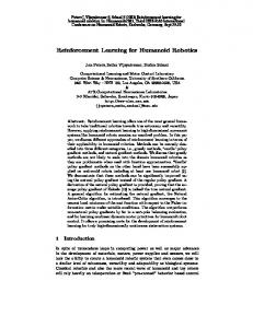
3 Problem Formulation In order to test the suitability of RL to the maintenance scheduling problem, it is necessary to define some indicative scenarios which can form the basis of simulated experiments. These simulations will involve two interacting components, a plant-model and a reinforcement learning model. The plant model provides the RL module with an indication of a current condition, the RL module then decides whether to execute a particular maintenance task. This is similar to the optimal control scenario described by Sutton, Barto and Williams [36] and is

M.J. Knowles, D. Baglee and S. Wermter

4

illustrated in figure 1 below. If maintenance is not performed then a failure may or may not occur. If the plant does not fail then a profit is returned as a reward. If the system does fail then a repair cost is deducted from the profit. If the RL module decides to perform maintenance then the system will not fail but a maintenance cost is deducted from the profit. The maintenance cost is considerably lower than the failure cost as is typical in real world scenarios. Thus at each time step the RL module must decide between a known, moderate reward by performing maintenance or risking no maintenance which could incur either a high reward in the event of no failure or a low reward if the plant fails STATE: age, condition Plant Model Age Condition Costs

DECISION: maintain / do not maintain

RL Module Q-Values Decisions

REWARD: profit / loss

Fig. 1. Simulation Architecture

3.1 Plant model The objective is to maximise reliability, i.e. the rate at which the equipment in question suffers a failure. In mathematical terms, the reliability function R(t) represents the likelihood that a system will run for a given time t without failure:

Rt

PT ! t

(3)

where T is the failure time. In the experiments described below, the plant model consists of a reliability function which is based on various combinations of variables including: x Time since last maintenance, t. It is assumed in all cases that the likelihood of a failure increases with t.

The Application of Reinforcement Learning to Optimal Scheduling of Maintenance

5

x Condition, c, which represents the condition of the plant, independent of the time since the last maintenance. After maintenance the value of condition is set to 1, and will decrease by a random amount after each time step. The likelihood of failure is inversely proportional to the value of c. For implementation purposes the reliability function is formulated in terms of the failure probability which is a function of the above variables, and represents the probability that a failure will occur for a given state (t,c). Several failure probability functions are used in the following experiments to illustrate various levels of complexity. These functions are given in the following section. Once the decision whether to maintain has been taken, the plant model will calculate the reward as described above based on the profit, repair cost and maintenance cost. In some cases the profit will also reduce at each time step to simulate the effects of increasing running costs (i.e. due to increased energy consumption etc) due to deteriorating condition. Once again various functions are used to illustrate different types of system, the functions are given for each experiment in the following section.

3.2 Reinforcement Learning Model In order to develop a maintenance model based on Q-Learning it is necessary to define the system state, the available actions and the Q function. The objective is to present the system with a stimulus and ask it a question, before providing reward based on the answer. In the experiments performed, the stimulus will be a set of state variables from the plant model which will consist of time since last maintenance, t, and condition, c. The response will be a decision to perform maintenance or not based on these state variables alone. This decision will be biased by the Q-Values for the two actions. Thus even if there is a larger expected reward, represented by a larger Q-value, available for a given action it is still possible for the other action to be taken in order to gain an opportunity to explore new actions. .Once the maintenance decision has been passed back to the plant model, the RL module will receive its reward. Based upon this reward the Q value for the selected action in the given state is updated according to equation 4:





Qst , at m Qst , at  D rt 1  J max Qst 1 , a  Qst , at a

(4)

It should be emphasised that the RL module only sees the state variables and reward which in a real-world application are measurable. The RL module has no knowledge of the reliability function or reward functions of the plant model.

M.J. Knowles, D. Baglee and S. Wermter

6

Actions are selected with the probabilities of maintenance actions being in direct proportion to the relative Q-Values. In order to ensure convergence, it is necessary for the value of  to decrease through the course of the trials subject to certain conditions [42,43]. This is achieved using the typical scheme:

D s , a

1 ns, a

(5)

Where n(s,a) represents the number of times Q(s,a) is visited.

3.3 Experiments In order to examine the performance of the RL algorithm in the maintenance scheduling scenario, four simulated experiments were performed using Matlab and these are described below. The first scenario presented is the most basic with the level of complexity increasing thereafter. In order to quantify the performance of the reinforcement learning system two metrics are used. The expected reward is calculated by running in validation mode 10000 times between each training iteration of the learning algorithm and averaging the reward accrued. Validation mode involves using the current policy to operate the plant starting from t = 0. Since the purpose of these tests is to measure the performance of a particular policy, there is no explorative behaviour in validation mode, i.e. the action with the highest Q-Value in a given state will always be selected. There is no learning or update of the Q-Value in validation mode. The other metric used is the Mean Time Between Failures (MTBF) which is a commonly used reliability metric. There are various formulations of MTBF, in this instance it represents the mean number of epochs between each occasion the system fails in validation mode.

4 Results 4.1 Level 1: Basic Model Here a simple system involving a running cost and a failure/repair cost is simulated. While this system is simplified it serves as an effective demonstrator of the application and as an introduction to the more elaborate, realistic scenarios below. The details are as follows. The system is capable of making a profit of 100

The Application of Reinforcement Learning to Optimal Scheduling of Maintenance

7

units at each epoch. The system has a failure probability of 0 which increases linearly by 0.05 each epoch as described in equation 6:

p fail t 0.05t

(6)

The reward available at each epoch is given by:

rt

­100 ° ®100  cr °100  c m ¯

no maintenance or failure no maintenance performed, system fails

(7)

maintenance performed

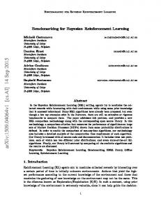
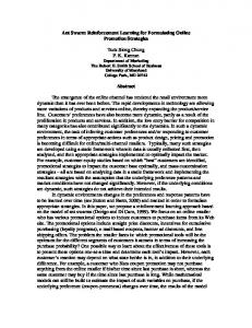
where cr = 120 represents the repair cost when the system fails and cm = 30 is the maintenance cost. The system is simulated for 1000 epochs. In this instance, the decision as to whether or not to perform maintenance is taken randomly for training purposes. The system was tested with the reward discount factor  set to 0.1. This value was determined empirically and found to be successful. The resulting Q-Values are shown in figure 2. It can be seen that maintenance becomes a more favorable option after 4 epochs. This is significant since the expected rewards for the two actions, calculated statistically using equations 6 and 7, are equal at 5 epochs with maintenance having a higher value than no maintenance before 5 epochs and a lower value after, as shown in table 1. Figure 3 shows the expected reward which can be seen to quickly converge, and the MTBF. It can be seen that the dominant MTBF is not the optimal value achieved. This is due to the agent attempting to achieve optimal long-term reward by delaying maintenance as long as it considers prudent.

Fig. 2. Q-Values for Level 1

M.J. Knowles, D. Baglee and S. Wermter

8 Table 1. Expected Rewards

T

pfail(t)

E(rt|maintenance)

E(rt|no maintenance)

1

0.05

70

94

2

0.1

70

88

3

0.15

70

82

4

0.2

70

76

5

0.25

70

70

6

0.3

70

64

7

0.35

70

58

Fig. 3. Average Reward and MTBF for Level 1

4.2 Level 2: Condition Data Here we provide the system with a measure of its current condition. The failure probability function is now modified to involve the condition variable c as discussed above and is shown in equation 8.

p fail t , c t

max 0.2  0.05t ,1  ct

(8)

The value of condition is updated at each time step as described in equation 9.

ct ct  1  0.1rand

(9)

The Application of Reinforcement Learning to Optimal Scheduling of Maintenance

9

Where rand represents a uniformly distributed random number in the range 01. The reward function remains as specified in equation 7. The results of the simulation can be seen in figure 4. It can be seen that the algorithm successfully converges on a policy yielding an average reward in the region of 81 units. Again, the final value of MTBF is suboptimal, however the optimal value corresponds with a lower level of reward which is the criteria against which the algorithm is optimising.

Fig. 4. Average Reward for Level 2.

4.3 Level 3: Energy Consumption Data

This scenario involves the simple reliability function from Level 1 as described by equation 6. Here, however, the running costs of the system increase at each time step to simulate an increase in energy usage due to a deteriorating condition. This is distinct from the above condition scenario where the running costs are not directly influenced until the equipment fails. Thus the profit available at each epoch reduces by 5 units at each time step after maintenance as described by equation 10.

rt

­100  5t ° ®100  5t  c r °100  c m ¯

no maintenance or failure no maintenance performed, system fails maintenance performed

(10)

The Q-values are shown in figure 5, average reward and MTBF in figure 6. It can be seen that the average reward converges, but on occasion loses its optimality temporarily. This appears to occur in the unlikely event of multiple successive failures in the learning algorithm but is rapidly corrected. The previously observed phenomenon regarding the sub-optimal MTBF is clearly illustrated here as the

10

M.J. Knowles, D. Baglee and S. Wermter

MTBF rises during periods where the policy becomes sub-optimal in terms of reward.

Fig. 5. Q-Values for Level 3.

Fig. 6. Average Reward for Level 3.

It should be noted that the effect of a deteriorating condition does not necessarily need to be formulated in terms of direct running costs. The reward offered could be formulated in terms of emissions, cost or other requirements scaled with suitable coefficients to give priority as chosen by the user.

4.4 Level 4: Complex System

In this scenario we combine the above concepts of time since last maintenance, condition measurement and energy usage. Thus the reliability function from Level 2 (equation 8) is used in conjunction with the reward function from level 3 (equation 10). The average reward and MTBF for level 4 are shown in figure 7. As with the previous examples, it can be seen that convergence is achieved.

The Application of Reinforcement Learning to Optimal Scheduling of Maintenance

11

Fig. 7. Average Reward for Level 4.

5 Discussion and Conclusions A number of benefits of RL have been demonstrated in limited yet realistic scenarios. The approach described has a number of merits including no requirement for any form of internal model and an ability to optimize against a number of criteria and could be applied successfully in a larger maintenance management application. The state described here comprises of the time since last maintenance and simple condition measurements, however the two variables used in the state vector cover the most important factors in a system’s reliability and potential improvements to the model would only improve the level of detail represented. The state-space could, for example, be expanded to include factors such as indicators of individual component condition, overall age, more detailed service history etc. As the state space becomes larger, maintaining an estimate of each and every possible Q-Value becomes problematic for scaling the problem size. This can be mitigated by modeling the Q-Function using a function approximator such as a neural network. This is an approach which has been successfully applied in many applications [12,13,44]. The repertoire of actions could be increased to consider different levels of maintenance, each with different availabilities. Future work in this area will need to probe these questions and address issues including the reliability of such a system in terms of the stability of the Q-Values, the effect of varying the future discount parameter to regulate how long-term the systems decision criteria is and the successful integration of cost based rewards with other parameters against which maintenance should be optimised such as MTBF. Furthermore the needs of industry in developing this application into a useful tool need to be considered to ensure it remains relevant. Issues such as formulating and observing the inner state of the system and the implications of the actual Q-Values in terms of metrics used by maintenance managers such as Return on Investment (ROI) will need to be addressed.

12

M.J. Knowles, D. Baglee and S. Wermter

References

1. Grall A., Berenguer C., Dieulle L.: A condition-based maintenance policy for stochastically deteriorating systems. Reliability Engineering & System Safety, Volume 76, Issue 2, Pages 167-180, ISSN 0951-8320, DOI: 10.1016/S0951-8320(01)00148-X.(2002) 2. Bengtsson M.: Standardization Issues in Condition Based Maintenance. In Condition Monitoring and Diagnostic Engineering Management - Proceedings of the 16th International Congress, August 27-29, 2003, Växjö University, Sweden, Edited by Shrivastav, O. and AlNajjar, B., Växjö University Press, ISBN 91-7636-376-7. (2003) 3. Davies A. (Ed): Handbook of Condition Monitoring - Techniques and Methodology. Springer, 1998 978-0-412-61320-3.(1997) 4. Barron R. (Ed): Engineering Condition Monitoring: Practice, Methods and Applications. Longman, 1996, 978-0582246560.(1996) 5. Wang W.: A model to determine the optimal critical level and the monitoring intervals in condition-based maintenance. International Journal of Production Research, volume 38 No 6 pp 1425 – 1436. (2000) 6. Meier A.: Is that old refrigerator worth saving? Home Energy Magazine http://homeenergy.org/archive/hem.dis.anl.gov/eehem/93/930107.html(1993) 7. Litt B., Megowen A. and Meier A.: Maintenance doesn’t necessarily lower energy use. Home Energy Magazine http://homeenergy.org/archive/hem.dis.anl.gov/eehem/93/930108.html. (1993) 8. Techato K-A, Watts D.J. and Chaiprapat S.: Life cycle analysis of retrofitting with high energy efficiency air-conditioner and fluorescent lamp in existing buildings. Energy Policy, Vol. 37, pp 318 – 325. (2009) 9. Boardman B., Lane K., Hinnells M., Banks N., Milne G., Goodwin A. and Fawcett T.: Transforming the UK Cold Market Domestic Equipment and Carbon Dioxide Emissions (DECADE) Report. (1997) 10. Knowles M.J. and Baglee D.:The Role of Maintenance in Energy Saving, 19th MIRCE International Symposium on Engineering and Managing Sustainability - A Reliability, Maintainability and Supportability Perspective, (2009) 11. Singh, S. Litman, D., Kearns M ., and Walker,M. Optimizing Dialogue Management with Reinforcement Learning: Experiments with the NJFun System. In Journal of Artificial Intelligence Research (JAIR),Volume 16, pp. 105-133. (2002) 12. Altahhan A., Burn K. Wermter S.: Visual Robot Homing using Sarsa(), Whole Image Measure, and Radial Basis Function. Proceedings IEEE IJCNN (2008) 13. Altahhan A.: Conjugate Temporal Difference Methods For Visual Robot Homing. PhD Thesis,University of Sunderland. (2009) 14. Lazaric, A., M. Restelli, Bonarini A.: Reinforcement Learning in Continuous Action Spaces through Sequential Monte Carlo Methods. Twenty First Annual Conference on Neural Information Processing Systems – NIPS. (2007) 15. Sheynikhovich, D., Chavarriaga R., Strosslin T. and Gerstner W.: Spatial Representation and Navigation in a Bio-inspired Robot. Biomimetic Neural Learning for Intelligent Robots. S. Wermter, M.Elshaw and G.Palm, Springer: 245-265. (2005) 16. Asadpour, M. and Siegwart, R.: Compact Q-learning optimized for micro-robots with processing and memory constrains. Robotics and Autonomous Systems, Science Direct, Elsevier. (2004) 17. Knowles, M.J. and Wermter, S.: The Hybrid Integration of Perceptual Symbol Systems and Interactive Reinforcement Learning. 8th International Conference on Hybrid Intelligent Systems. Barcelona, Spain, September 10-12th, (2008) 18. Muse, D. and Wermter, S.: Actor-Critic Learning for Platform-Independent Robot Navigation. Cognitive Computation, Volume 1, Springer New York, pp. 203-220, (2009)

The Application of Reinforcement Learning to Optimal Scheduling of Maintenance

13

19. Weber, C., Elshaw, M., Wermter, S., Triesch J. and Willmot, C.: Reinforcement Learning Embedded in Brains and Robots, In: Weber, C., Elshaw M., and Mayer N. M. (Eds.) Reinforcement Learning: Theory and Applications. pp. 119-142, I-Tech Education and Publishing, Vienna, Austria. (2008) 20. Stone, P., Sutton R. S. and Kuhlmann G.: Reinforcement learning for robocup soccer keepaway. International Society for Adaptive Behavior 13(3): 165–188 (2005) 21. Taylor M.E. and Stone P.: Towards reinforcement learning representation transfer. In The Autonomous Agents and Multi-Agent Systems Conference (AAMAS-07), Honolulu, Hawaii. (2007) 22. Kalyanakrishnan S., Liu Y. and Stone P.: Half Field Offense in RoboCup Soccer: A Multiagent Reinforcement Learning Case Study. Lecture Notes In Computer Science, Springer (2007) 23. Lokuge, P. and Alahakoon, D.: Reinforcement learning in neuro BDI agents for achieving agent's intentions in vessel berthing applications 19th International Conference on Advanced Information Networking and Applications, 2005. AINA 2005. Volume: 1 Digital Object Identifier: 10.1109/AINA.2005.293, Page(s): 681 - 686 vol.1(2005) 24. Cong Shi, Shicong Meng, Yuanjie Liu, Dingyi Han and Yong Yu: Reinforcement Learning for Query-Oriented Routing Indices in Unstructured Peer-to-Peer Networks, Sixth IEEE International Conference on Peer-to-Peer Computing P2P 2006, Digital Object Identifier: 10.1109/P2P.2006.30, Page(s): 267 - 274 (2006) 25. Cong Shi, Shicong Meng, Yuanjie Liu, Dingyi Han and Yong Yu: Reinforcement Learning for Query-Oriented Routing Indices in Unstructured Peer-to-Peer Networks, Sixth IEEE International Conference on Peer-to-Peer Computing, 2006. P2P 2006.Digital Object Identifier: 10.1109/P2P.2006, Page(s): 267 - 274 (2006). 26 Mattila, V.: Flight time allocation for a fleet of aircraft through reinforcement learning. Simulation Conference, 2007 Winter, Digital Object Identifier: 10.1109/WSC.2007.4419888 Page(s): 2373 - 2373 (2007) 27. Zhang, Y. and Fromherz, M.: Constrained flooding: a robust and efficient routing framework for wireless sensor networks, 20th International Conference on Advanced Information Networking and Applications, 2006. AINA 2006.Volume: 1 Digital Object Identifier: 10.1109/AINA.2006.132 (2006) 28. Chasparis, G.C. and Shamma, J.S.: Efficient network formation by distributed reinforcement 47th IEEE Conference on Decision and Control, 2008. CDC 2008. Digital Object Identifier: 10.1109/CDC.2008.4739163, Page(s): 1690 - 1695 (2008). 29. Usynin, A., Hines, J.W. and Urmanov, A.: Prognostics-Driven Optimal Control for Equipment Performing in Uncertain Environment Aerospace Conference, 2008 IEEE Digital Object Identifier: 10.1109/AERO.2008.4526626, Page(s): 1 – 9 (2008) 30. Lihu, A.and Holban, S.: Top five most promising algorithms in scheduling. 5th International Symposium on Applied Computational Intelligence and Informatics, 2009. SACI '09. Digital Object Identifier: 10.1109/SACI.2009.5136281, Page(s): 397 - 404 (2009). 31. Zhang Huiliang and Huang Shell Ying: BDIE architecture for rational agents.. International Conference on Integration of Knowledge Intensive Multi-Agent Systems, Page(s): 623 - 628 (2005) 32. Malhotra, R., Blasch, E.P. and Johnson, J.D.: Learning sensor-detection policies ., Proceedings of the IEEE 1997 National Aerospace and Electronics Conference, 1997. NAECON 1997Volume: 2 Digital Object Identifier: 10.1109/NAECON.1997.622727 , Page(s): 769 - 776 vol.2 (1997) 33. Sutton, R.S. and Barto, A.G.: Reinforcement Learning: An Introduction, IEEE Transactions on Neural Networks Volume: 9 , Issue: 5 Digital Object Identifier: 10.1109/TNN.1998.712192, Page(s): 1054 - 1054 (1998) 34. Barto, A.G.: Reinforcement learning in the real world 2004. Proceedings. 2004 IEEE International Joint Conference on Neural Networks, Volume: 3 (2004)

14

M.J. Knowles, D. Baglee and S. Wermter

35. Barto, A.G. and Dietterich, T.G.: Reinforcement Learning and Its Relationship to Supervised Learning In Si, J., Barto, A.G., Powell, W.B., and Wunsch, D., editors, Handbook of Learning and Approximate Dynamic Programming, pages 47 - 64. Wiley-IEEE Press, (2004) 36. Sutton, R.S., Barto, A.G.: and Williams, R.J.: Reinforcement learning is direct adaptive optimal control Control Systems Magazine, IEEE Volume: 12 , Issue: 2 Digital Object Identifier: 10.1109/37.126844 Publication Year: 1992 , Page(s): 19 - 22 37. Kaebling, L.P., Littman, M.L. and Moore A.W.: Reinforcement Learning: A Survey. Journal of Artificial Intelligence Research, Vol 4, pp 237 – 285. (1996) 38. Watkins, C.J.C.H.: Learning from Delayed Rewards. PhD thesis, Cambridge University, Cambridge, England. (1989). 39. Rummery G.A and Niranjan M.: On-line Q-Learning using connectionist Systems. Technical Report CUED/F-INFENG/TR166, Cambridge University. (1994) 40. Sutton, R.: Learning to predict by the methods of temporal differences. Machine Learning 3 (1),pp 9–44. doi:10.1007/BF00115009. (1988) 41. Foster D.J., Morris, R.G.N.and Dayan, P.: A model of hippocampally dependent navigation, using the temporal learning rule. Hippocampus, Vol. 10, pp. 1-16, (2000) 42. Humphrys, M.: Action Selection methods using Reinforcement Learning , PhD thesis, University of Cambridge, Computer Laboratory (1997) 43. Watkins, C.J.C.H. and Dayan, P.: Technical Note: Q-Learning, Machine Learning 8:279-292. (1992) 44 Sutton R.S.: Generalization in Reinforcement Learning: Successful Examples Using Sparse Coarse Coding. Advances in Neural Processing Systems 8, pp1038 – 1044. (1996)