Application of Runge-Kutta method for the solution of ... - ScienceDirect

Application of Runge-Kutta method for the solution of non-linear partial differential equations Ashok Kumar Department

qf Mechunical

Onturio, Cunadu

Engineering,

University

?f’ Waterloo, Waterloo,

and T. E. Unny Department qf Cicil Engineering, Canudu (Received 23 March 1976)

University

c~f Wrrterloo.

Waterloo,

Ontario.

The application of RungeKutta methods as a means of solving non-linear partial differential equations is demonstrated with the help of a specific fluid flow problem. The numerical results obtained are compared with the analytical solution and the solution obtained by implicit, explicit and Crank-Nicholson finite difference methods. The error analysis and computational efficiency analysis are performed to test each method. The inherent advantages and disadvantages in the context of the problem considered are discussed. Limitations of the Runge-Kutta method are also given.

Introduction RungeeKutta method is a powerful tool for the solution of ordinary differential equations (ODE). Most of the research has been oriented towards improving the accuracy or the flexibility (to accommodate problems of diverse nature) of the classical Rungee Kutta method’-‘. In this study the solution of a class of non-linear partial differential equations (PDE) is obtained by using this method. A similar approach has been taken by Rushton’ and Marino and Yeh’ in the analysis of aquifer systems. A particular problem of this type describing the transient flow of a gas through porous media is investigated. The equation representing this phenomenon is non-linear in nature. A summary of previous work on the solution of PDEs is given by Sinovec and Madsen”. This paper illustrates a method of lines” and presents its application to seven different problems. The software PDPONE” uses a subroutine called GEARB” (non-stiff portion of which is based on AdamsBashforth-Moulton Predictor-Corrector method) for numerical integration. The present paper uses a Runge-Kutta scheme, and in addition, provides a detailed comparison of the solutions with those

obtained analytically as well as those from various finite-difference schemes14.15. User’s computer requirements differ and, in this connection. a discussion of the computing times and computer space requirements are very helpful. These are the points that are emphasized in this paper. The study shows that the solution of non-linear PDE is feasible by the Runge-Kutta method; it yields more accurate results than that obtained by finite difference methods for the example considered here. The use of Runge-Kutta methods to solve problems of this type is a novel approach. It is anticipated that this technique can be utilized to solve other complex problems of a similar nature.

Development of governing equations The horizontal transient flow of a gas through porous media can be expressed by general equations as: Continuity equation* :

4%+ (V . PC,) *Nomenclature

s=

0

(1)

IS given at the end of the paper.

Appl. Math. Modelling,

1977, Vol 1, March

199

Runge-Kutta

method

for the solution

of non-linear

PDEs: A. Kumar and T. E. Unny

Darcy’s equation:

Thus, what follows is applicable to the problem and boundary conditions considered and the results may be different with other boundary conditions. For example, equation (3) represents one-dimensional diffusion equation in a stationary atmosphere (no wind velocity) if r is eddy diffusivity, fi = 1, (BT/M)S(t, x) is the source strength and P is concentration field. Equations (3)-(j) with the parameters defined by the set of equations (6) are solved by the Runge-Kutta and finite difference schemes.

Incorporating the assumption that the gas law is applicable (i.e. PL’ = nzRT and p = nM/V) and the flow is one-dimensional, in the above equations, the following partial differential equation is obtained:

‘[ 1

& .iP)E +gh(t,X,= P(P) (g Oo

= g (‘i.fJ

BT

S

(12)

i.e.,

t>o

=o

=

where the increment function, 4, is a suitably chosen approximation to the function f(P, t) over the interval P, < P G P,+l. The problem at hand may be posed as a system of ODE by partial discretization of equation (3) as follows:

OGXGL

= pi

P(L.t) = g(t) dP

method

(5)

The values selected for various parameters functions are the same as used by Culham i.e.,

and and Varga16

(13) where.

L = 10000ft. P, = 4000 lb/in’ k=

(absolute)

(6)

1mD

4’ = 0.2 (7)

(8)

(,x(1

_

e-+z!i dr2

,f’(u)= (;i’(o.x

1

- ;)

(9) (10)

The discussion will be carried along with this specific problem of fluid flow. The basic expression (equation 3), though considered here only in the context of pressure distribution in porous media, also represents heat transfer and diffusion phenomena with appropriate choice of parameters.

200

Appl. Math.

Modelling,

1977,

Vol. 1, March

(16)

The first term of equation (3) is not only non-linear, but also contains a second derivative of the coefficient derivative product. This term results from the situation where the diffusion or dispersion coefficient, x(P), is a function of pressure and therefore must be considered in the second derivative. This quantity [s(P)] must be computed at successive intervals of time to ensure that a numerical scheme continues to be stable for the complete execution of the programme. The vector ODE given by equation (13) has been solved for the unknown pressure vector using fourth order RK method with Gill’s modification1%15. This modification has the advantage of compensation for accumulated round-otl’ error and less storage requirements than the other RK formulae. The numerical results will be discussed later on while the treatment of boundary conditions follows. Discretization of the derivative boundary condition at x = 0 is done either by off-centred or reflection

Runge-Kutta

approximation approximations approximation

for the solution

4Pi+,

-

Pi+2 2h

x=0=

3Pi

of non-linear

PDEs:

A. Kumar

and

T. E. Unny

where

(for details see Appendix I). Both the are of second order. The off-centred for this problem may be expressed as:

l3P ax

method

0

o

(17)

---=

lb, _ 1

i.e., Pi =

4pi+l

-

‘0,

pi+2

3

The reflection yields:

approximation,

ap pi+l =---------~ ax,=,

-

on the other hand,

pi-l

0

(18)

2h

i.e., Pi,1

= Pi_1

1

and 2 is a vector of known quantities. It should be noted that the explicit scheme (equation 2) does not yield a tridiagonal matrix F but an identity matrix. As an example the elements of coefficient matrix F and vector li for implicit scheme are given in Appendix II. For other methods, one can easily derive these elements from the original equations. Once a numerical scheme is expressed in the form of equation (23), a software (computer program) utilizing a subroutine based on Thomas algorithm provides the solution for unknown pressure vector pi,,+ 1

Finite difference methods Various numerical schemes are available for the solution of partial differential equations’ 7--22. The non-linear terms of equation (3) present some difficulty in choosing a particular finite difference scheme. To illustrate the application of finite difference schemes for this problem, the explicit, the implicit and the Crank-Nicholson (C-N) methods are selected. The finite difference forms of equation (3) for each method may be written as: Explicit

scheme at u point (i,n)

(19) Implicit

scheme at a point (i,n)

9tpi,n+1) + Crank-Nicholson

gsi.n+

1 =

B(pi,n)6tpi,n

(20)

scheme at a point (i,n):

+ = B(pi,n)dtpi,n

k

$tsi.n+l

+

si,n)

(21)

where,

(22) and the difference operator 2 is defined by equation (14). For discretization of the derivative boundary condition at X = 0. equation (12) or (13) may be used. However, the reflection method of approximation (equation 13) is preferred with the implicit scheme because it yields a symmetric tridiagonal matrix. Also the reflection approximation has been used for the explicit and C-N method. After substitution of the initial and boundary conditions, equations (19) to (21) may be written for unknown pressure in the following general matrix form : (23)

Convergence, stability and compatibility A numerical method is said to be convergent if the exact solution of the difference equation p (without round-off error) tends to the solution of the partial differential equation P as Ax and At both tend to zero. The difference (P - p) is called the discretization error. In general, the discretization error can be decreased by decreasing Ax and Ar. This means that the number of equations to be solved will increase and the method will be restricted by such factors as time, labour, degree of accuracy desired, computer core capacity etc. For non-linear problems the conditions under which a scheme is convergent are not yet known except in a few particular cases because the final expression for the discretization error is generally in terms of unknown derivatives for which no upper and lower bounds can be estimated. Further discussion will be given after discussing stability and compatibility. A system of finite difference equations is stable when the cumulative effect of all the rounding errors is negligible. In some cases, it is quite possible to develop this system, a stable system but which has a solution that converges to the solution of a different boundary value problem as the grid spacing tends to zero. Such a difference scheme is said to be incompatible or inconsistent with the partial differential equation. Generally, for linear problems if the conditions of stability and compatibility are satisfied by the numerical method under consideration, then the scheme is said to be convergent. The stability and compatibility may also imply convergence for a non-linear problem. In order to test convergence the following points were considered (based on above discussion): (1) For RK method the control of accuracy and adjustment of the step size At is done by comparison of the results due to double and single step size 2 Ar and Ar23. This is one of the many methods available in the literature for this purpose’.3,15,24. (2) Each scheme under consideration satisfies the condition of compatibility For all cases, in order to make sure that steps Ax

Appl. Math. Modelling,

1977,

Vol 1, March

201

Runge-Kutta

3

method

for the solution

of non-linear

PDEs: A. Kumar and T. E. Unny

t

z* - - - --

//+

=

5

!Jx_l

TimeIdays)

At

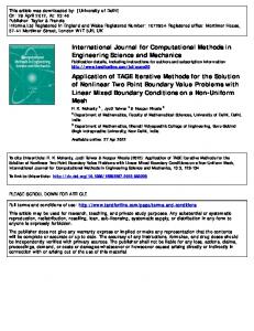
figure 7 Average error. Runge-Kutta; V, explicit;

Time (days)

= 1.0 day. 0,

0.

l.

Implicit,

C-N

and Af are correct, a number of step sizes are selected to find a stable range for the parameters and then the appropriate step size in each direction is chosen keeping in mind: (a) for RK method the condition outlined in (1): (b) for explicit method y = 1/2l* where y is defined as: At

‘1=p*p(p)

Further.

the variations

in cc(p)and /I(p) require

2.5

At 0.

= 1 .O day. 0,

Implicit;

0,

C-N

t

and C-N

Computer runs* were made with various combinations of parameters (h, At, and number of days) and the results were compared with the analytical solution”. The percentage error was computed for each method. The average error (I, norm) is shown in Figure 1. The lx -norm of the error (transient error) at the interior points of the grid network is plotted in Figure 2; while the spatial distribution of the error for each case is depicted in Figure 3. With continued experimentation it is possible that a reduced percentage error could have been obtained. Although the error in Figures I, 2 and 3 is shown for ten days, the behaviour of these plots may be projected for visualization of the error for a time greater than ten days. These Figures, also, give an idea (quantitatively) about the improvement in results obtained by RK method as compared to finite difference methods. A low profile for spatial distribution of error (Figure 3) along the entire length of the core favours. especially for the situations where *All computations were performed University of Waterloo Computing

Math.

on IBM Center.

Modelling,

360:system

1977,

c

that

Results and Discussion

Appl.

2 Transient error Runge-Kutta; V, explicit;

4~)

(c) for linear problems. the implicit method method are unconditionally stable.

202

Figure

of the

Vol. 1, March

5.01 0

5000

Distance

10000

(ft.)

figure 3 Spatial distribution of error. Time LL t = 1 .O day. 0. Implicit; 0, Runge-Kutta; 0. C-N

= 5.0 days; V. explicit;

pressure P is a critical parameter, the RK method over finite difference methods. Thus the RK approach is applicable for the solution of non-linear PDE. For this problem. the C-N scheme is superior than the explicit scheme and implicit scheme. However, the RK approach possesses the advantage of higher order accuracy (also see Table I) (4th order in time for RK scheme. and 2nd order in time for both finite difference methods) and automatic step size, At, adjustment. Other important points that have been used in comparison of various computing techniques are computing time and core storage (computer memory) requirement. Table 1 provides a data base for this purpose. Though the execution time and core storage requirements in the RK method are more than the finite difference methods, the error committed by the

Runge-Kutta Table

1

Comparison

method

of computing

for the solution

* 1 unit

= z

CPU

Core

Reader

Printer

8(h2 e(h= 0(hz 0(/r=

2.57 1.61 1.49 1.70

0.48 0.31 0.29 0.33

0.39 0.15 0.14 0.17

0.60 0.34 0.33 0.36

x CPU time

A. Kumar

and

T. E. Unny

P) T) T) ?)

Total

time for costing*

Order of approximation + + + +

PDEs:

time Computing

RK method Implicit method Explicit method C-N method

of non-linear

execution time (min)

0.22 0.13 012 0.14

in minutes

+ 0.0021* PRT lines + 0.007’ cards punched + 0.0015’ cards read

+ o,058 1000 + 2~.

ERT

1200

where

R

= kilobytes

of core and ERT

=

60’

CPU(min)

former method is far less than the latter ones (see Figure 1 and Table I). From the point of view of computational efficiency explicit method seems to be the ‘best’. However. the time required for each finite difference increases several times whenever an attempt is made to obtain the results of same accuracy as that of RK method. The implicit and C-N finite difference schemes are unconditionally stable while the explicit one is conditionally stable. as discussed earlier. The sensitivity to the boundary conditions is delayed by one step in the explicit scheme because the evaluation of pressure at any point does not require the use of neighbouring points at the same level of time. The error contributed by the boundary condition approximation is the same for all methods considered and better results may be obtained by using irregular grid network2’. Another aspect that can be considered in favour of both the approaches is relatively minimal technical expertise on the part of the user as compared with other approaches e.g.. analog/hybrid simulation. The RK method may not work satisfactorily in those cases where initial and boundary conditions (given by equation 4) are not ‘smooth’ in nature. Typical examples are: (1) the boundary condition P(L,t) = g(t), changes abruptly from one time step to another. In such cases the selection of large time step will not be justified: (2) the initial condition P(x,O) is a step function in x. In this case, the regular grid (Ax) will introduce large error: (3) the boundary condition P(O,t) is a sinusoidal function in t. It is interesting to note that the conclusions drawn in this paper on RK method in the solution PDE agree with the work of Sincovec and Madsen” even though a different method is used for integrations.

+ 0.027

* //O count

type methods. As observed by the authors the RungeKutta approach yields better results and to overcome the limitations of this method the area of irregular grid network should be investigated.

Nomenclature Conversion factor. A = 158.07” i? Conversion factor. B = 1696.41 lh g(t) Boundary condition at X = L Grid spacing along X-axis II Permeability. mD k Length of the core. ft L Molecular weight. lbmilb mole M Pressure. Ib/in.2 (absolute) P Density P Generation term, lbm/ft3 day S Absolute temperature. R 7 Time Space coordinate ; Compressibility factor. dimensionless Grid spacing in time direction ht I-1 Viscosity. cP Porosity 4’ A

0

Order of magnitude Difference operator: Difference operator:

Y 6

see equation see equation

(14) (22)

Subscript of grid point in X-direction. 1.2....1 + 1;l = L/h Subscript of grid point in r-direction. 1,2.3,...N + I:&‘= totaltime/Ar

i n

i =

n =

Conclusions The equation of transient flow of an ideal gas through porous media, as an example of a class of non-linear PDE. has been considered. The solution of the problem has been obtained by using two distinct approaches, viz., the RungeeKutta methods and the finite difference

References I 2 3 4

Gill. S. Pux~. Crrr7&v/&c Phil. Sot. 195 I. 47. 96 Call, D. H. and Reeves. R. F. Co~?r~un. ACM, 1958. 5, 39 Collatz, L. ‘The Numerical Treatment of Difl’erential Equationa’. Springer-Verlag. Berlin. 1960 Scraton, R. E. Conq~ur. J. 1964. 7, 246

Appl.

Math. Modelling,

1977,

Vol. 1, March

203

Runge-Kutta

12 13 14 I5 16 I7 I8 I9 20

21 22 23 24 25

method

for the solution

of non-linear

Chai. A. S. Sirnulrrrron 1970. 15. 89 Chai, A. S. Si~trulcrtion 1972, 18. 21 Schiesser. W. E. Proc~. iY71 Su~irtnc~ Cu~rtpt,~~erSirntrlorron Cwzf. 1972, p 202 Rushton, K. R. J. H~drol. 1973. 18, I Marino, M. A. and Yeh. W. W. G. J. H~drol. 1973. 20. 255 Sincovec, R. F. and Madsen. N. K. AC,M Trtms. Mrrrlt. Sofiirrrrr 1975. 1. 232 Madsen. N. K. and Sincovec. R. F. in Computational Methods in Nonlinear Mechanics’, (Ed. J. T. Oden (‘I r/l.) Texas Inst. for Computational Mechanics. Austin, 1974 Sincovec. R. F. and Madsen N. K. AC&f Tr~ns. Mtrtll. Sqfin;urr 1975, 1. 261 Hindmarsh, A. C. Rep. ACID-3005Y Lawrence Livermore Lab.. Livermore. 1973 Mitchell, A. R. ‘Computational Methods in Partial Diflerential Equations’, John Wiley. New York. 1969 Carnaham, B.. Luther, H. A. and Wilkes. J. 0. ‘Applied Numerical Methods’, .lohn Wiley. New York. 1969 Culham. W. E. and Varga, R. S. SPE Pqw No. ?XO6, AfME T~~.lY/.Y I 970 Ralston, A. and Wilf. H. S. ‘Mathematical Methods for Digital Computers’, John Wiley, New York. 1962 Ames, W. F. ‘Numerical Methods for Partial Differential Equations’. Nelson. London. 1969 Lapidus. L. ‘Digital Computation for Chemical Engineers’. McGraw-Hill, New York. 1962 Marcal, P. V. in ‘Numerical Solution of Partial Differential Equations’, Vol II, (Ed. B. Hubbard). Academic Press. New York, 1971 Cardenas. A. F. and Karplus, W. _I_Corirrnun. AC!14 1970, 13, 184 Richtmyer. R. D. ‘Difference Methods for Initial-Value Problems’, Interscience. New York. 1957 System:360 SSP Manual. IBM Corporation. New York. 1970 System;360 Continuous System Modeling Program-User’s Manual, IBM Corporation, New York. 1972 Snyder, L. J. SPE J. 1969 (June). p 170

PDEs: A. Kumar and

T. E. Unny

where, 0(/t’) signifies that the discretized expression for aP/8xli is a second order approximation. The expression for reflection approximation of c’P/c?x at a point i may similarly be derived by expressing pressure P, in terms of P, _ 1 and P, + , . Thus: Pi = Pi-,

+ /,g

+ ;

2

+ H(P)

(A4)

I

4 = P,+1 From

equations

(A3 (A4) and (A5), one obtains:

P c7P - P._, _ =r+lI_ 2h i?.Xi

+ tl(h2)

Appendix II The elements of matrix for the implicit method ai = 1 + *“Zi;P,

F and vector zin are derived as:

equation

n)[pi,.+ I(%+ 1129 +

xi-

(23)

1,2,u)l (1 < i G I)

bi =

-

*x2i;pi

n)[pi+

Ia+

1 . %+

1/2,nl

Appendix I The derivation for discretized form of ZP/i-x with so-called off-centred and reflection approximations is shown in this Appendix. The off-centred approximation of BP/ax at a point i may be obtained by expressing the pressure Pi in terms ofPi+, and Pi+2 with the help of Taylor series, i.e., (Al)

(A2) Multiplying equation (Al) by 4 and then subtracting from equation (A2), one obtains (after rearranging the terms) : ll?P

4P,+r

ax ;

204

Appl. Math.

- P,+2 - 3Pi 2h

Modelling,

+ 0th’)

1977,

(A3)

Vol 1, March

At di = Pi,, + E M ‘~+‘+’ (lG’