Application of Stacked Convolutional and Long Short-Term Memory Network for Accurate Identification of CAD ECG Signals Jen Hong Tana, Yuki Hagiwaraa, Winnie Panga, Ivy Lima, Shu Lih Oha, Muhammad Adama, Ru San Tanb,c, Ming Chena, U Rajendra Acharyaa,d,e,* a
Department of Electronics and Computer Engineering, Ngee Ann Polytechnic, Singapore. b c d
National Heart Centre Singapore, Singapore.
Duke-National University of Singapore Medical School, Singapore.
Department of Biomedical Engineering, School of Science and Technology, Singapore University of Social Sciences, Singapore.
e
Department of Biomedical Engineering, Faculty of Engineering, University of Malaya, Malaysia. *Corresponding Author: Postal Address: Department of Electronics and Computer Engineering, Ngee Ann Polytechnic, Singapore 599489. Telephone: +65 6460 6135; Email Address:
[email protected]
ABSTRACT Coronary artery disease (CAD) is the most common cause of heart disease globally. This is because there is no symptom exhibited in its initial phase until the disease progresses to an advanced stage. The electrocardiogram (ECG) is a widely accessible diagnostic tool to diagnose CAD that captures abnormal activity of the heart. However, it lacks diagnostic sensitivity. One reason is that, it is very challenging to visually interpret the ECG signal due to its very low amplitude. Hence, identification of abnormal ECG morphology by clinicians may be prone to error. Thus, it is essential to develop a software which can provide an automated and objective interpretation of the ECG signal. This paper proposes the implementation of long short-term memory (LSTM) network with convolutional neural network (CNN) to automatically diagnose CAD ECG signals accurately. Our proposed deep learning model is able to detect CAD ECG signals with a diagnostic accuracy of 99.85% with blindfold strategy. The developed prototype model is ready to be tested with an appropriate huge database before the clinical usage.
Keywords – coronary artery disease; convolutional neural network; deep learning; electrocardiogram signals; long short-term memory; PhysioNet database.
1
1. Introduction According to the American College of Cardiology, cardiovascular diseases contribute to one-third of all deaths worldwide [28]. In 2015, more than 400 million people globally were diagnosed with cardiovascular disease. Cardiovascular diseases are significant contributors to global increased mortality rates [28]. For this reason, there is a need to develop a cost-effective and efficacious approach to alleviate this global issue. Generally, cardiovascular diseases are categorized into three groups: circulatory, electrical, and structural [17]. Coronary artery disease (CAD) (circulatory-related disease involving the coronary circulation) is the most common form of cardiovascular disease [9, 28]. CAD occurs through a process called atherosclerosis, which is a disorder caused by build-up of plaque in the inner walls of the coronary arteries [9]. The plaque consists of fatty or cholesterol deposits and its accumulation will constrict blood flow through the arteries. Furthermore, as the plaque builds up, blood flow through the arteries decreases and eventually the heart muscle receives insufficient oxygen-rich blood supply [9]. Over time, the plaque may solidify and rupture. This activates circulating platelets in the blood, resulting in the formation of blood clots on the surface of the plaque That may potentially occluded the vessel entirely, and block off blood flow [12]. An entirely blocked coronary artery may trigger off heart attack (myocardial infarction) [1, 4, 7]. In addition, chronic CAD may result in heart muscle damage, weakening of heart muscle, and lead to other cardiovascular diseases such as arrhythmias [3, 5] and heart failure [12]. The early stage of CAD normally produces no symptoms until the disease progresses into an advanced stage. Pre-symptomatic health check-ups may unearth early disease and avert further progression of the disease with timely treatment. The electrocardiogram (ECG) is a widely accessible diagnostic tool that records the electrical activity of the heart [25]. ECG signals can also be obtained during exercise stress test where the ECG signals are recorded when the subject is undergoing a physical stress [10, 11]. In addition, heart rate variability (HRV) signals can be extracted from ECG signals [6, 15, 20, 27, 30]. Other common diagnostic tests include echocardiography, which uses sound waves to produce visual images of the heart in order to detect structural heart abnormality [31, 32]. Still, the ECG technique is the prime choice for the primary assessment of the heart as it is cost-effective, easy to implement, and noninvasive. Manual diagnosis of ECG signals is however very challenging and tedious as the signals vary morphologically (see Figure 1). Also, manual analysis of the ECG signals which is currently the
2
clinically standard practice might be subject to inter-observer variability among different clinicians [24]. Thus, a computer-aided diagnosis system is initiated to overcome these limitations of visual inspection of ECG signals. There are numerous works proposed on the computerized decision support using ECG signals to diagnose the different types of heart conditions [2, 8, 22, 26]. Table 1 shows the various studies conducted on the automated detection of CAD using ECG signals. Kumar et al. [22] developed an automated system to differentiate CAD and normal ECG signals with an accuracy of 99.60%. They decomposed the ECG beats with flexible analytic wavelet transform, and then statistically significant features extracted were fed into the classifier for classification. Acharya et al. [8] compared the performance of higher order bi-spectrum and cumulant features to categorize normal versus CAD ECG beats. They also formulated 2 CAD indexes from the extracted bi-spectrum and cumulant features to numerically characterize the two classes of ECG signals based on a single number. Later, Acharya et al. [2] came up with an improved algorithm. They designed an 11-layer deep convolutional neural network (CNN) to classify ECG signals into normal and CAD classes. Their model attained an accuracy of 94.95% and 95.11% with 2-second and 5-second ECG segments respectively without any hand-engineered features extraction and selection processes. Oh et al. [26] employed the common spatial pattern technique to extract significant features from decomposed ECG segments. These features were then fed into a k-nearest neighbor classifier for classification. They reported a high diagnostic sensitivity and specificity of 99.64% and 99.71% respectively with an accuracy of 99.65%. Although the proposed technique achieved the maximum performance, this approach used many features. The works by Kumar et al. [22], Oh et al. [26], and Acharya et al. [8] adopted the traditional machine learning process of features extraction, features selection, and classification. In this work, a stacked long short-term memory (LSTM) [18] network with CNN [23] is proposed to classify normal versus CAD ECG signals. LSTM is known to be well-suited for the processes and prediction of time-series signals. However, the computation performed in LSTM is generally slower.
3
In this study our algorithm first slices a 5 seconds ECG segment (with 1,285 data points) into 211 short segments. Each short segment consists of 24 data points. Instead of simply feeding these 211 short segments into layers of LSTM, we perform 2 rounds of 1D convolution-maxpooling to extract the significant features in these segments. The resultant output is a set of 50 short segments, with each segment comprising 32 data points. This process reduces the amount of data points for computation in LSTM (CNN for most of the time runs faster than LSTM). These segments are then fed to 3 layers of LSTM and a fully-connected layer to perform the diagnosis. To the best of our knowledge, in literature there is no similar structure proposed and applied on the classification of normal and CAD ECG signals. There were deep neural network architectures (which used CNN and LSTM) proposed for the classification of atrial fibrillation [34]. However, in their work they first converted an ECG signal into a logarithmic spectrogram and then followed by a series of 2D convolutions. Whereas in this work, we perform 1D convolution (as defined in [19]) and 1D maxpooling (as defined in [19]) before we send features to LSTM.
Table 1: Selected studies on the automated detection of CAD using ECG signals obtained from the same database. Performances (%) Number of ECG Authors Year Techniques data Sensitivity Specificity Accuracy Kumar et al.
2017
[22]
Normal: 137,587 CAD: 44,426
• Flexible analytic
99.57
99.61
99.60
Cumulant:
Cumulant:
Cumulant:
97.75
99.39
98.99
Bi-
Bi-
Bi-
spectrum:
spectrum:
spectrum:
94.57
99.34%
98.17
wavelet transform
(lead II, ECG
• Kruskal-Wallis test
beats)
• Student t-test • Least square support vector machine classifier • Ten-fold crossvalidation
Acharya et al. [8]
2017a
Normal: 137,587 CAD: 44,426 (lead II, ECG beats)
• Higher-order statics and spectra • Bispectrum and cumulant features • Principal component analysis • K-nearest neighbor classifier • CAD indexes developed • Ten-fold crossvalidation
4
Acharya et al.
2017b
[2]
Net A –
• 11 layers CNN
Net A:
Net A:
Net A:
Normal: 80,000
• Net A (2-seconds) and
93.72
95.18
94.95
Net B:
Net B:
Net B:
91.13
95.88
95.11
99.64
99.71
99.65
99.85
99.84
99.85
CAD: 15,300
Net B (5-seconds) • Ten-fold cross-
Net B –
validation
Normal: 32,000 CAD: 6,120 (lead II, ECG segments) Oh et al.
2017
[26]
Normal: 3,791 CAD: 12,308 (12 leads, ECG segments)
• Wavelet packet decomposition • Common spatial pattern • K-nearest neighbor classifier • Ten-fold crossvalidation
Present study
2017
Normal: 32,000 CAD: 6,120 (lead II, ECG
• 8-layers stacked CNNLSTM • Blindfold
segments)
2. Data Used The ECG data used in this work were obtained from an open source PhysioNet database [16]. The normal and CAD ECG data were downloaded from Fantasia and St Petersburg Institute of Cardiology Technics 12-leads arrhythmia respectively. Only lead II ECG signals were used for this study. The ECG data used were collected from 7 CAD (6 females and 1 male) and 40 normal (20 females and 20 males) subjects. The ECG signals were cut into segments of 5 seconds with each segment containing 1,285 data points. Figure 1 shows examples of normal and CAD ECG segments. The 40 normal subjects yielded 32,000 segments of ECG signals and the 7 CAD subjects produced 6,120 ECG segments. We have used two approaches to validate our method: i.
First validation approach:
This validation approach was a non-subject specific. The ECG segments were randomly shuffled, and 10% (3,200 normal and 612 CAD) of the ECG segments were used for training and 90% (28,800 normal and 5,508 CAD) of the ECG segments were used for testing.
5
ii.
Second validation approach:
This approach uses subject specific data whereby the first 12,000 normal ECG segments were used for training (roughly equivalent to 15 subjects’ ECG data) and the remaining segments were used for testing (20,000 ECG segments). The first 2,600 CAD ECG segments were used for training (roughly equivalent to 3 subjects’ ECG data) and the remaining segments were used for testing (3,520 ECG segments).
Figure 1: Samples of normal and CAD 5-second ECG segments.
3. Methodology A stacked CNN-LSTM model is proposed in this study to classify the ECG data into their respective classes.
3.1 Pre-processing The CAD and normal ECG data were sampled at frequencies of 257 Hz and 250 Hz respectively. To ensure consistency between the two classes of signals, the normal ECG data was up-sampled to 257 Hz. After which, the ECG data was subjected to discrete wavelet transform (Daubechies 6, mother wavelet) for noise removal and baseline wander [29]. Subsequently, the ECG data were
6
segmented into 5-second time intervals without performing the R-peak detection of the ECG signals. In this work we did not directly use the above processed signals for training. Instead we generated a pool of 32,000 normal and 32,000 CAD ECG segments by the following augmentation procedures: i.
Re-normalize a processed ECG segment with a randomly determined mean and standard deviation using z-transform.
ii.
Generate a sinusoidal signal with a starting phase at random from -180° to -90° and an ending phase at random from 90° to 180°; the amplitude is set randomly between ± 2 (normalized value).
iii.
Produce a random Gaussian noise signal with a mean of 0 and standard deviation of 0.05.
iv.
Combine the above three signals to produce the new signal.
Furthermore, for every generated signal, we sliced the 1D signal into 211 shorter segments. Each short segment consists of 24 data points. The slicing was done in the following fashion: for every 6th data point in the signal, we extracted 24 consecutive sample points from the point of interest (inclusive of the point of interest). These short segments were put together into a 2D matrix and fed into CNN.
3.2 Convolutional Neural Network (CNN) The CNN architecture in this consists 2 convolution layers and 2 maxpooling layers with stride (the amount by which the filter slides at a time) of 1 and 2 respectively: (i)
Convolution: This layer operates the convolution between the kernel and the input ECG segments to obtain the feature map (output). This process picks up characteristic features from the ECG samples.
(ii)
Pooling: This layer down-sample the dimensions of the output shape to minimize overfitting and computational cost, while retaining the characteristic features from the ECG samples.
7
3.3 Long Short-Term Memory (LSTM) Network Unlike feedforward network, the LSTM is a recurrent neural network (RNN) that has an input, hidden (memory block), and an output layer. The memory block contains 3 gate units namely the input, forget, and output with a self-recurrent connection neuron [18]. (i)
Input gate: learns what information is to be stored in the memory block.
(ii)
Forget gate: learns how much information to be retained or forgotten from the memory block.
(iii)
Output gate: learns when the stored information can be used.
3 stacked LSTM networks were employed in the architecture.
3.4 Architecture of the CNN-LSTM Model
Figure 2: The proposed network structure. The dimension of the output from every block is detailed within the parenthesis.
8
Figure 2 illustrates the proposed architecture and Table 2 summarizes the detail involved in the structure. Layers 1 to 4 are convolutional layers and layers 5 to 7 are LSTM layers. The last layer is a fully-connected layer which makes the classification (CAD versus normal ECG class). The CNN was used as a feature extractor and the LSTM network as a sequential learning.
Table 2: Proposed net structure in this work. Layers
Type
0
Input
211 x24
-
-
Number of trainable parameters 0
1
1D Convolution
207 x 40
5 x 24
1
2
1D Maxpooling
103 x 40
2x1
3
1D Convolution
101 x 32
4
1D Maxpooling
5
Output shape
Kernel (filter) size
Recurrent dropout
Dropout
-
-
4,840
-
-
2
0
-
-
3 x 40
1
3,872
-
-
50 x 32
2x1
2
0
-
-
LSTM
50 x 32
-
-
8,320
0.25
0.5
6
LSTM
50 x 16
-
-
3,136
0.25
-
7
LSTM
4
-
-
336
-
-
8
Fully-connected
1
-
-
5
-
-
Total
20,509
Stride
The input to the net is a 211 x 24 matrix. It was convolved with a 5 x 24 kernel to form an output shape of 207 x 40. Maxpooling operation was applied to reduce the feature map into a matrix of 103 x 40 (layer 2). After which, another round of convolution and maxpooling were performed in layers 3 and 4. The output from the layer 4 (50 x 32) then went through three LSTMs (layer 5, 6, 7), and fully connected to layer 8 (output layer), which has only a single output shape to determine the class of the input ECG segment. A sample output of layer 3 corresponding to Figure 1 is illustrated in Figure 3 and Figure 4. A total of 32 plots (feature map) can be seen with each plot representing an output vector (total output shape: 101 x 32). The plots were generated from the convolution with a 3 x 40 kernel and a stride of 1. The plots are visual features learned after the 2nd convolution operation. It can be noted that these plots are unique for normal and CAD ECG signals. Similarly, Figure 4, shows the 32 output plots. However, it is noted that the plots look more repetitive as compared to the
9
plots in Figure 3. This is because the heartbeat in a regular and healthy heart is more regular and hence, the features learned by each operation are more consistent. The net was trained using ‘Adam’ algorithm with the default parameters setting [20]. It was trained with a batch size of 512 over 100 epochs. A blindfold [13] approach was used to test the proposed model with the test data from non-patient specific and from the patient specific test data.
10
Figure 3: Illustration of layer 3 output of a sample CAD ECG segment with output shape of 101 x 32.
11
Figure 4: Illustration of layer 3 output of a sample normal ECG segment with output shape of 101 x 32.
12
4. Results
The stacked convolutional LSTM network is developed and trained using Keras with Theano backend [33]. It was trained on a workstation with two Intel Xeon, 2.20 GHz (E5-2650v4) processor and a 512 GB RAM with a Quadro K4200, 4 GB memory GPU. It took approximately 51 seconds to run a single epoch. Table 3 shows the confusion matrix for the classification of CAD and normal ECG segments using first validation approach (non-subject specific). Very small percentage of 0.16% of the normal segments were misclassified as CAD class and 0.15% of the CAD ECG segments were misclassified as normal ECG segments. It can be noted that very high diagnostic accuracies were obtained with just a small number of training samples. The overall performances are documented in Table 4. The recall (sensitivity) values for normal and CAD are 0.9984 and 0.9985 respectively. Table 5 shows the confusion matrix for the classification of the ECG segments using second validation approach (subject specific). Nearly 0.8% of the normal ECG segments were misclassified into CAD class and 23.44% of CAD ECG segments were grouped as normal ECG segments. It can also be observed that more CAD ECG segments were categorized wrongly. This may be due to the limited number of CAD ECG data used to train the algorithm as there were approximately 4.6 times more normal than CAD ECG data used to train the proposed model. Hence, in Table 6, it is noted that the recall for CAD is 76.56% whereas the recall for normal ECG segments is 99.13%. Also, the overall performance obtained with the proposed model is recorded in Table 6. A high accuracy percentage of 99.14% is achieved in the correct detection of normal ECG segments and an accuracy of 76.56% is yielded in the correct categorization of CAD ECG segments. The overall diagnostic accuracy of 95.76% is obtained.
Original
Table 3: Confusion matrix of the algorithm performance using the test data (non-subject specific data). Predicted Normal CAD Total Normal CAD
28,755
45
28,800
8
5,500
5,508 34,308
13
Table 4: The classification performance in this work (non-subject specific data). Precision Recall F1-score Accuracy (%) Normal
0.9997
0.9984
0.9991
99.84
CAD
0.9919
0.9985
0.9952
99.85
Total
0.9985
0.9985
0.9952
99.85
Original
Table 5: Confusion matrix of the algorithm performance using the test data (subject specific data). Predicted Normal CAD Total Normal CAD
19,827
173
20,000
825
2,695
3,520 23,520
Table 6: The classification performance in this work (subject specific data). Precision Recall F1-score Accuracy (%) Normal
0.9601
0.9913
0.9755
99.14
CAD
0.9397
0.7656
0.8438
76.56
Total
0.9570
0.9576
0.9557
95.76
5. Discussion It is observed that high diagnostic performances were yielded from conventional techniques [8, 22, 26]. Even though they have obtained remarkably high performance with advanced signal processing techniques, our proposed model does not require R-peak detection as compared to their methods. Furthermore, the published papers recorded in Table 1 have performed the tenfold cross-validation in their studies whereas, in this work, a blindfold strategy was implemented. Nevertheless, the proposed model achieved the highest performance out of these shallow learning techniques. Also, the proposed deep learning approach eliminates the reliance on features engineering as some of the features extracted by hand may be data dependent. In addition, a subject specific classification was also performed to validate the proposed network (see Tables 5 and 6). A high diagnostic accuracy of 95.76% was obtained. In our opinion, the most
14
appropriate and accurate method to validate the proposed model is to use subject specific data for training and testing. Hence, two validation approaches were implemented in this study. In this work, a combination of CNN with stacked LSTM in a single network model was proposed so that the overall performance of the model can be optimized through training. Both CNN and LSTM models learn different functions and hence, merging of these two nets has yielded higher diagnostic accuracy [14]. In addition, the proposed CNN-LSTM network attained better diagnostic performance as compared to the 11-layers CNN model developed by Acharya et al. [2], for the same number of 5-seconds ECG segments used in this study (See Table 1). Nevertheless, it can be noted that no data augmentation was performed in their work. Hence, the data augmentation in this work has also helped improve the robustness of the proposed algorithm as it can generate more ECG segments with slight variations to train the model. A total of 64,000 (32,000 normal and 32,000 CAD) ECG segments were generated and fed into the proposed model for training. The advantages of the proposed model are: i.
Fully automated and requires minimum feature engineering.
ii.
It is robust as it has achieved a diagnostic accuracy of 95.76% with the blindfold strategy (for subject specific data).
iii.
Less computationally expensive when the LSTM is combined with CNN model.
The disadvantage of the proposed model is: i.
The limited number of CAD data yielded less variation in the ECG data. Hence, unable to achieve optimum diagnostic performance for subject specific data.
The authors intend to extend the proposed stacked CNN-LSTM network to the other cardiovascular diseases such as myocardial infarction and congestive heart failure. Ultimately, the authors plan to design an automated system which can diagnose the different types of cardiovascular diseases using one universal algorithm.
15
6. Conclusion In this study, a state-of-the-art algorithm (stacked CNN-LSTM) is employed to automatically diagnose CAD using ECG signals. The system is fully automatic and requires minimum handengineering to train the algorithm. We have obtained the highest diagnostic performance using 8-layer stacked CNN-LSTM network. Our system has the potential to be deployed in clinical settings to assist cardiologists to make objective and reliable diagnosis of ECG signals. Furthermore, the proposed algorithm can be installed in a portable device so that not only cardiologists but also other healthcare professionals and nurses can make use of this device to provide an accurate initial diagnosis of patients’ cardiovascular health during a routine health check-up. Utilizing this device may also help to reduce the rate of mortality due to CAD by diagnosing CAD early and providing patients with the appropriate preventive treatment. Also, this device can be employed in developing countries where availability of medical professionals is limited.
7. References 1. U. R. Acharya, H. Fujita, M. Adam, S. L. Oh, V. K. Sudarshan, J. H. Tan, J. E. W. Koh, Y. Hagiwara, K. C. Chua, K. P. Chua, R. S. Tan, “Automated characterization and classification of coronary artery disease and myocardial infarction by decomposition of ECG signals: a comparative study”, Information Sciences, vol. 377, pp. 17-29, 2017h. 2. U. R. Acharya, H. Fujita, S. L. Oh, M. Adam, J. H. Tan, K. C. Chua, “Automated detection of coronary artery disease using different durations of ECG segments with convolutional neural network”, Knowledge-Based Systems, vol. 132, pp. 62-71, 2017b. 3. U. R. Acharya, H. Fujita, S. L. Oh, Y. Hagiwara, J. H. Tan, M. Adam, “Automated detection of arrhythmias using different intervals of tachycardia ECG segments with convolutional neural network”, Information Sciences, vol. 405, pp. 81-90, 2017c. 4. U. R. Acharya, H. Fujita, S. L. Oh, Y. Hagiwara, J. H. Tan, M. Adam, “Application of deep convolutional neural network for automated detection of myocardial infarction using ECG signals”, Information Sciences, vol. 415, pp. 190-198, 2017d. 5. U. R. Acharya, H. Fujita, S. L. Oh, Y. Hagiwara, J. H. Tan, M. Adam, A. Gertych, R. S. Tan, “A deep convolutional neural network model to classify heartbeats”, Computers in Biology and Medicine, vol. 89, pp. 389-396, 2017e. 16
6. U. R. Acharya, H. Fujita, V. K. Sudarshan, S. L. Oh, A. Muhammad, J. E. W. Koh, J. H. Tan, K. C. Chua, K. P. Chua, R. S. Tan, “Application of empirical mode decomposition (EMD) for automated identification of congestive heart failure using heart rate signals”, Neural Computing and Applications, vol. 28, pp. 3073-3094, 2017f. 7. U. R. Acharya, H. Fujita, V. K. Sudarshan, S. L. Oh, A. Muhammad, J. H. Tan, J. H. Koo, A. Jain, C. M. Lim, K. C. Chua, “Automated characterization of coronary artery disease, myocardial infarction, and congestive heart failure using contourlet and shearlet transforms of electrocardiogram signal”, Knowledge-Based Systems, vol. 132, pp. 156-166, 2017g. 8. U. R. Acharya, V. K. Sudarshan, J. E. W. Koh, R. J. Martis, J. H. Tan, S. L. Oh, M. Adam, Y. Hagiwara, M. R. K. Mookiah, K. P. Chua, K. C. Chua, R. S. Tan, “Application of higherorder spectra for the characterization of coronary artery disease using electrocardiogram signals”, Biomedical Signal Processing and Control, vol. 31, pp. 31-43, 2017a. 9. American Heart Association, “What is cardiovascular disease?”, retrieved from http://www.heart.org/HEARTORG/Support/What-is-CardiovascularDisease_UCM_301852_Article.jsp#.WgOf5VuCzIU, 2017. 10. I. Babaoglu, O. Findik, M. Bayrak, “Effects of principal component analysis on assessment of coronary artery diseases using support vector machine”, Expert Systems with Applications, vol. 37(3), pp.2182-2185, 2010a. 11. I. Babaoglu, O. Findik, E. Ulker, “A comparison of feature selection models utilizing binary particle swarm optimization and genetic algorithm in determining coronary artery disease using support vector machine”, Expert Systems with Applications, vol. 37(4), pp.3177-3183, 2010b. 12. Centers for Disease Control and Prevention, “Coronary artery disease (CAD)”, retrieved from https://www.cdc.gov/heartdisease/coronary_ad.htm, 2015. 13. L. P. Devroye, T. J. Wagner, “Distribution-free performance bounds for potential function rules”, IEEE Transactions on Information Theory, vol. 25, no. 5, pp. 601-604, 1979. 14. K. J. Geras, A. Mohammed, R. Caruana, G. Urban, S. Wang, O. Aslan, M. Philipose, M. Richardson, C. Sutton, “Blending LSTMs into CNNs”, arXiv:1511.06433, 2015. 15. D. Giri, U. R. Acharya, R. J. Martis, S. V. Sree, T. C. Lim, T. A. VI, J. Suri, “Automated diagnosis of coronary artery disease affected patients using LDA, PCA, ICA, and discrete wavelet transform”, Knowledge-Based Systems, vol 37, pp. 274-282, 2013.
17
16. A. L. Goldberger, L. A. N. Amaral, L. Glass, J. M. Hausdorff, P. C. Ivanov, R. G. Mark, J. E. Mietus, G. B. Moody, C. K. Peng, H. E. Stanley, “Physiobank, physiotoolkit, and physionet: components of a new research resource for complex physiologic signals”, Circulation, vol. 101(23), pp. E215-E220, 2000. 17. Heart
Rhythm
Society,
“Heart
diseases
and
disorders”,
retrieved
from
http://www.hrsonline.org/Patient-Resources/Heart-Diseases-Disorders. 18. S. Hochreiter, J. Schmidhuber, “Long short-term memory”, Neural Computation, vol. 9, pp. 1735-1780, 1997. 19. Keras: The python deep learning library, retrieved from https://keras.io/. 20. D. P. Kingma, J. Ba, “Adam: a method for stochastic optimization”, Proceedings of the 3rd International Conference on Learning Representations, 2014. 21. M. Kumar, R. B. Pachori, U. R. Acharya, “An efficient automated technique for CAD diagnosis using flexible analytic wavelet transform and entropy features extracted from HRV signals”, Expert Systems with Applications, vol. 63, pp. 165-172, 2016. 22. M. Kumar, R. B. Pachori, U. R. Acharya, “Characterization of coronary artery disease using flexible analytic wavelet transform applied on ECG signals”, Biomedical Signal Processing and Control, vol. 31, pp. 301-308, 2017. 23. Y. LeCun, Y. Bengio, “Convolutional networks for images, speech, and time-series”, In The handbook of brain theory and neural networks, MIT Press Cambridge, MA, USA, 1998. 24. R. J. Martis, U. R. Acharya, H. Adeli, “Current methods in electrocardiogram characterization”, Computers in Biology and Medicine, vol. 48(1), pp. 133-149, 2014. 25. Mayo
Clinic
Staff,
“Coronary
artery
disease,
diagnosis”,
retrieved
from
https://www.mayoclinic.org/diseases-conditions/coronary-artery-disease/diagnosistreatment/drc-20350619, 2017. 26. S. L. Oh, M. Adam, J. H. Tan, Y. Hagiwara, V. K. Sudarshan, J. E. W. Koh, K. C. Chua, K. P. Chua, R. S. Tan, E. Y. K. Ng, “Automated identification of coronary artery disease from short-term 12 lead electrocardiogram signals by using wavelet packet decomposition and common spatial pattern techniques”, Journal of Mechanics in Medicine and Biology, vol. 17(7), pp. 1740007 (19 pages), 2017. 27. S. Patidar, R. B. Pachori, U. R. Acharya, “Automated diagnosis of coronary artery disease using tunable-Q wavelet transform applied on heart rate signals”, Knowledge-Based Systems, vol. 82, pp. 1-10, 2015. 18
28. G. A. Roth, C. Johnson, A. Abajobir, F. Abd-Allah, S. F. Abera, G. Abyu, M. Ahmed, B. Aksut, T. Alam, K. Alam, F. Alla, N. Alvis-Guzman, S. Amrock, H. Ansari, J. Arnlov, H. Asayesh, T. M. Atey, L. Avila-Burgos, C. Murray, “Global, regional, and national burden of cardiovascular diseases for 10 causes, 1990 to 2015”, Journal of the American College of Cardiology, vol. 70(1), pp. 1-25, 2017. 29. B. N. Singh, A. Tiwari, “Optimal selection of wavelet basis function applied to ECG signal denoising”, Digital Signal Processing, vol. 16(3), pp. 275-287, 2006. 30. S. Sood, M. Kumar, R. B. Pachori, U. R. Acharya, “Application of empirical mode decomposition-based features for analysis of normal and CAD heart rate signals”, Journals of Mechanics in Medicine and Biology, vol. 16(1), pp. 1640002 (20 pages), 2016. 31. V. K. Sudarshan, U. R. Acharya, E. Y. K. Ng, R. S. Tan, S. M. Chou, D. N. Ghista, “An integrated index for automated detection of infarcted myocardium from cross-sectional echocardiograms using texton-based features (part 1)”, Computers in Biology and Medicine, vol. 71, pp. 231-240, 2016a. 32. V. K. Sudarshan, U. R. Acharya, E. Y. K. Ng, R. S. Tan, S. M. Chou, D. N. Ghista, “Data mining framework for identification of myocardial infarction stages in ultrasound: a hybrid feature extraction paradigm (part 2)”, Computers in Biology and Medicine, vol. 71, pp. 241-251, 2016b. 33. The Theano Development Team, “Theano: a python framework for fast computation of mathematical expressions”, https://arxiv.org/pdf/1605.02688.pdf. 34. M. Zihlmann, D. Perekrestenko, M. Tschannen, “Convolutional recurrent neural networks for electrocardiogram classification”, arXiv:1710.06122v1, 2017.
19