Ensemble Application of Convolutional Neural Networks ... - SenticNet

Ensemble Application of Convolutional Neural Networks and Multiple Kernel Learning for Multimodal Sentiment Analysis Soujanya Poriaa , Haiyun Pengb , Amir Hussaina , Newton Howardc , Erik Cambriab,d a Department

of Computing Science and Mathematics, University of Stirling, UK of Computer Science and Engineering, Nanyang Technological University, Singapore c Computational Neuroscience and Functional Neurosurgery, University of Oxford, UK d Corresponding author

b School

Abstract The advent of the Social Web has enabled anyone with an Internet connection to easily create and share their ideas, opinions and content with millions of other people around the world. In pace with a global deluge of videos from billions of computers, smartphones, tablets, university projectors and security cameras, the amount of multimodal content on the Web has been growing exponentially, and with that comes the need for decoding such information into useful knowledge. In this paper, a multimodal affective data analysis framework is proposed to extract user opinion and emotions from video content. In particular, multiple kernel learning is used to combine visual, audio and textual modalities. The proposed framework outperforms the state-of-the-art model in multimodal sentiment analysis research with a margin of 10-13% and 3-5% accuracy on polarity detection and emotion recognition, respectively. The paper also proposes an extensive study on decision-level fusion.

1. Introduction Subjectivity detection and sentiment analysis consist of the automatic identification of the human mind’s private states, e.g., opinions, emotions, moods, behaviors and beliefs [1]. In particular, the former focuses on classifying sentiment data as either objective (neutral) or subjective (opinionated), while the latter aims to infer a positive or negative polarity. Hence, in most cases, both tasks are considered binary classification problems. To date, most of the work on sentiment analysis has been carried out on text data. With a videocamera in every pocket and the rise of social media, people are now making use of videos (e.g., YouTube, Vimeo, VideoLectures), images (e.g., Flickr, Picasa, Facebook) and audio files (e.g., podcasts) to air their opinions on social media platforms. Thus, it has become critical to find new methods for the mining of opinions and sentiments from these diverse modalities. Plenty of research has been carried out in the field of audio-visual emotion recognition. Some work has also been conducted on fusing audio, visual and textual modalities to detect emotion from videos. However, a unique common framework is still missing for both tasks. There are also very few studies combining textual clues with audio and visual features. This leads to the need for more extensive research on the use of these three channels together. This paper aims to solve the two key research questions given below • Is a common framework useful for both multimodal emotion and sentiment analysis? • Can audio, visual and textual features jointly enhance the performance of unimodal and bimodal emotion and sentiment analysis classifiers?

Email addresses: [email protected] (Soujanya Poria), [email protected] (Haiyun Peng), [email protected] (Amir Hussain), [email protected] (Newton Howard), [email protected] (Erik Cambria)

Preprint submitted to Elsevier

January 28, 2017

Studies conducted in the past lacked extensive research [2, 3, 4] and very few of them clearly described the extraction of features and fusion of the information extracted from different modalities. In this paper, we discuss the feature extraction process from different modalities in detail and explain how to use such features for multimodal affect analysis. The YouTube dataset originally developed by [5] and the IEMOCAP dataset [6] were used to demonstrate the accuracy of the proposed framework. We used several supervised classifiers for the sentiment classification task: the CLM-Z [7] based method was used for feature extraction from visual modality; the openSMILE toolkit was used to extract various features from audio; and finally, textual features were extracted using a deep convolutional neural network (CNN). The fusion of these heterogeneous features was carried out by means of multiple kernel learning (MKL) using support vector machine (SVM) as a classifier with different types of kernel. The rest of the paper is organized as follows: Section 2 proposes motivations behind this work; Section 3 discusses related works on multimodal emotion detection, sentiment analysis and multimodal fusion; Section 4 describes the used datasets in detail; Sections 5, 6 and 7 explain how visual, audio, and textual data are processed, respectively; Section 8 proposes experimental results; Section 9 proposes a faster version of the framework; finally, Section 10 concludes the paper. 2. Motivations The research in this field is rapidly picking up and has attracted the attention of academia and industry alike. Combined with advances in signal processing and AI, this research has led to the development of advanced intelligent systems that intend to detect and process affective information contained in multimodal sources. However, the majority of such state-of-the-art frameworks rely on processing a single modality, i.e., text, audio, or video. Additionally, all of these systems are known to exhibit limitations in terms of meeting robustness, accuracy, and overall performance requirements, which, in turn, greatly restricts the usefulness of such systems in real-world applications. The aim of multi-sensor data fusion is to increase the accuracy and reliability of estimates [8]. Many applications, such as navigation tools, have already demonstrated the potential of data fusion. These illustrate the importance and feasibility of developing a multimodal framework that could cope with all three sensing modalities – text, audio, and video in human-centric environments. Humans communicate and express their emotions and sentiments through different channels. Textual, audio, and visual modalities are concurrently and cognitively exploited to enable effective extraction of the semantic and affective information conveyed in conversation [9]. People are gradually shifting from text to video to express their opinion about a product or service, as it is now much easier and faster to produce and share them. For the same reasons, potential customers are now more inclined to browse for video reviews of the product they are interested in, rather than looking for lengthy written reviews. Another reason for doing this is that, while reliable written reviews are quite hard to find, it is sufficient to search for the name of the product on YouTube and choose the clips with most views in order to find good video reviews. Finally, videos are generally more reliable than written text as reviewers often reveal their identity by showing their face, which also allows viewers to better decode conveyed emotions [10]. Hence, videos can be an excellent resource for emotion and sentiment analysis but the medium also comes with major challenges which need to be overcome. For example, expressiveness of opinion varies widely from person to person [2]. Some people express their opinions more vocally, some more visually and others rely exclusively on logic and express little emotion. These personal differences can help guide us towards the affect seeking expression. When a person expresses his or her opinions with more vocal modulation, the audio data will often contain most of the clues indicative of an opinion. When a person is highly communicative via facial expressions, most of the data needed for opinion mining may often be determined through facial expression analysis. So, a generic model needs to be developed which can adapt itself for any user and provide a consistent result. Both of our multimodal affect analysis models are trained on robust data containing opinions or narratives from a wide range of users. In this paper, we show that the ensemble application of feature extraction from different types of data and modalities is able to significantly enhance the performance of multimodal emotion and sentiment approach.

2

3. Related Work In this section, we discuss related works in multimodal affect detection covering both emotion and sentiment analysis. 3.1. Text based emotion and sentiment analysis Sentiment analysis systems can be broadly categorized into knowledge-based and statistics-based systems [11]. While the use of knowledge bases was initially more popular for the identification of emotions and polarity in text, sentiment analysis researchers have recently been using statistics-based approaches, with a special focus on supervised statistical methods. For example, Pang et al. [12] compared the performance of different machine learning algorithms on a movie review dataset and obtained 82.90% accuracy, using only a large number of textual features. A recent approach by Socher et al. [13] obtained even better accuracy (85%) on the same dataset using a recursive neural tensor network (RNTN). Yu and Hatzivassiloglou [14] used semantic orientation of words to identify polarity at sentence level. Melville et al. [15] developed a framework that exploits word-class association information for domain-dependent sentiment analysis. Other unsupervised or knowledge-based approaches to sentiment analysis include Turney et al. [16], who used seed words to calculate the polarity and semantic orientation of phrases; Melville et al. [17], who proposed a mathematical model to extract emotional clues from blogs and then used these for sentiment detection; Gangemi et al. [18], who presented an unsupervised frame-based approach to identify opinion holders and topics based on the assumption that events and situations are the primary entities for contextualizing opinions; and Cambria et al. [19], who proposed a multidisciplinary framework for polarity detection based on SenticNet [20], a concept-level commonsense knowledge base. Sentiment analysis research can also be categorized as single-domain [12, 16, 21, 22] or cross-domain [23]. The work presented in [24] discusses spectral feature alignment to group domain-specific words from different domains into clusters. They first incorporated domain-independent words to help the clustering process and then exploited the resulting clusters to reduce the gap between domain-specific words of two domains. Bollegala et al. [25] developed a sentiment-sensitive distributional thesaurus by using labeled training data from the source domain and unlabeled training data from both the source and target domains. Sentiment sensitivity was obtained by including documents’ sentiment labels into the context vector. At the time of training and testing, this sentiment thesaurus was used to expand the feature vector. The task of automatically identifying fine-grained emotions, such as anger, joy, surprise, fear, disgust, and sadness, explicitly or implicitly expressed in a text has been addressed by several researchers [26, 27]. There are a number of theories on emotion taxonomy which spans from Ekman’s emotion categorization model to the Hourglass of Emotion (Figure 1) [28]. So far, approaches to text-based emotion and sentiment detection rely mainly on rule-based techniques, bag of words modeling using a large sentiment or emotion lexicon [29], or statistical approaches that assume the availability of a large dataset annotated with polarity or emotion labels [30]. Several supervised and unsupervised classifiers have been built to recognize emotional content in texts [31]. The SNoW architecture [32] is one of the most useful frameworks for text-based emotion detection. In the last decade, researchers have been focusing on sentiment extraction from texts of different genres, such as product reviews [33], news [34], tweets [35], and essays [36], to name a few. 3.2. Audio Visual Emotion and Sentiment Analysis In 1970, Ekman et al. [37] carried out extensive studies on facial expressions. Their research showed that universal facial expressions are able to provide sufficient clues to detect emotions. They used anger, sadness, surprise, fear, disgust, and joy as six basic emotion classes. Such basic affective categories are sufficient to describe most of the emotions expressed by facial expression. However, this list does not include the emotion expressed through facial expression by a person when he or she shows disrespect to someone; thus, a seventh basic emotion, contempt, was introduced by Matsumoto [38]. The Active Appearance Model [39, 40] and Optical Flow-based techniques [41] are common approaches that use facial expression coding system (FACS) to understand facial expressions. Exploiting action units (AU) as features in well known classifier like k nearest neighbors, Bayesian networks, hidden Markov models (HMM), and artificial neural networks (ANN) [42] has helped many researchers to infer emotions from facial expression. The performance 3

Figure 1: The Hourglass of Emotion

of several machine-learning algorithms for detecting emotions from facial expressions is presented in Table 1 (cited from Chen et al. [43]). All such systems, however, use different, manually-crafted corpora, which makes it impossible to perform a comparative evaluation of their performance. To this end, recently Xu et al. [44] constructed a framework which takes color features from the superpixel of images and later a piece-wise linear transformation was used to learn the emotional feature distribution. The framework is basically a novel feature learning framework from emotion labeled set of images. Recent studies on speech-based emotion analysis [40, 51, 52, 53, 54] have focused on identifying several acoustic features such as fundamental frequency (pitch), intensity of utterance [43], bandwidth, and duration. The speakerdependent approach gives much better results than the speaker-independent approach, as shown by the excellent results of Navas et al. [55], where about 98% accuracy was achieved by using the Gaussian mixture model (GMM) as a classifier, with prosodic, voice quality as well as Mel frequency cepstral coefficients (MFCC) employed as speech features. When it comes to fusing audio-visual emotion recognition, two of the early works were done by De Silva et al. [56] and Chen et al. [57]. Both of these works showed that a bimodal system yielded a higher accuracy than any 4

Table 1: Performance of various learning algorithms for detecting emotions from facial images.

Method Lanitis et al.[39] Cohen et al. [45] Mase [46] Rosenblum et al. [47] Otsuka & Ohya [48] Yacoob & Davis [49] Essa & Pentland [50]

Processing Appearance Model Appearance Model Optical flow Optical flow 2D FT of optical flow Optical flow Optical flow

Classification algorithm Distance-based Bayesian network kNN ANN HMM Rule-based Distance-based

Accuracy 74% 83% 86% 88% 93% 95% 98%

unimodal system. More recent research on audio-visual emotion recognition has been conducted at either feature level [58, 59, 60] or decision level [61, 62, 63, 64]. Though there are plenty of research articles on audio-visual emotion recognition, only a few pieces of research works have been done on multimodal emotion or sentiment analysis using textual clues along with visual and audio modality. The works as described in [5, 4, 65] fused information from audio, visual and textual modalities to extract emotion and sentiment. Metallinou et al. [66] and Eyben et al. [67] fused audio and textual modality for emotion recognition. Both these approaches relied on feature-level fusion. Wu et al. [68] fused audio and textual clues at decision level. 3.3. Multiple Kernel Learning Several studies have reported that MKL outperforms the average kernel baselines. MKL is very similar to group LASSO which is a feature selection method where features are organized into groups. However, the choice of kernel coefficients can have a significant impact on the classification accuracy and efficiency of MKL [69]. For example, in Alzheimer’s disease patients, different types of tests correspond to different modalities that can reveal varied aspects of the diagnosis. MR images may show only a slight hippocampal atrophy while the FDGPET image may reveal increased hypometabolism suggestive of Alzheimer. In [70], MKL was used simultaneously for optimizing different modalities in Alzheimer’s disease. However, in order to deal with co-morbidity with other diseases, they used the hinge loss function to penalize misclassified samples that did not scale well with the number of kernels. Adaptive MKL (AdaMKL) was proposed in [71] based on biconvex optimization and Gaussian kernels. Here, the objective function alternatively learns one component at a time while fixing the others, resulting in an increased computation time. In [72], higher order kernels are used to enhance the learning of MKL. Here, block co-ordinate gradient optimization is used as it approximates the Hessian matrix of derivatives as a diagonal resulting in loss of information. MKL is also used in signal processing where grouping of features is useful to improve the interpretability of the learned parameters [73]. MKL was applied to a Polish opinion aggregator service that contained textual opinions of different products, but this study did not consider the hierarchical relation of different attributes of products [74]. Group-sensitive MKL for object recognition in images integrates a global kernel clustering method with MKL for sharing of group-sensitive information [75]. Hence, the two different kernels are used to group the training data and the kernels are aligned during optimization. They showed that their method outperformed baseline grouping strategies on the WikipediaMM dataset of real-world web images. The drawback of this method is that a looping strategy is used to relabel groups and may not reach the global optimum solution. MKL was used to detect the presence of a large lump in images using a convolution kernel [76]. However, they only considered Gaussian features for the images. In [77], MKL was used to combine and re-weight multiple features by using structured latent variables during video event detection [77]. Here, two different types of kernels are used to group global features and segments in the test video that are similar to the training videos. While, the results on TRECVID dataset of video events outperformed baselines, the method requires tuning of parameters and assumes random initialization of latent variables. Multimodal features were fused at different levels of fusion for the indexing of web data in [78]. The concept of kernel slack variables for each of the base kernels was used to classify YouTube videos in [79]. In order to select good features and discard bad features that may not be useful to the kernel, Liu et al. [80] used a beta prior distribution. 5

Table 2: Utterances per emotion class

Angry 1083

Happy 1630

Sad 1083

Neutral 1683

Total 5479

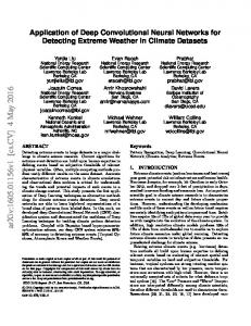
Recently, MKL with Fourier transform on the Gaussian kernels has been applied to Alzheimer’s Disease classification using both sMRI and fMRI images [81]. Researchers used L2 norm to enforce group sparsity constraints which were not robust on noisy datasets. Lastly, Online MKL shows good accuracy on object recognition tasks by extending online kernel learning to online MKL, however, the time complexity of the methods is dependent on the dataset [82]. 4. Dataset Used In this section, we describe the datasets used in multimodal sentiment and emotion analysis experiments. 4.1. Multimodal Sentiment Analysis Dataset For our experiment, we use the dataset developed by Morency et al. [2]. They started collecting the videos from popular social media (e.g., YouTube) using several keywords to produce search results consisting of videos of either product reviews or recommendation. Some of these keywords are my favorite products, non recommended perfumes, recommended movies etc. A total of 80 videos were collected in this way. The dataset includes 15 male and 65 female speakers, with their age ranging approximately from 20-60 years. The videos were converted to mp4 format with a standard size of 360x480. All videos were pre-processed to avoid the issues of introductory titles and multiple topics, and the length of the videos varied from 2-5 minutes. Many videos on YouTube contained an introductory sequence where a title was shown, sometimes accompanied with a visual animation. To address this issue, the first 30 seconds was removed from each video. Morency et al. [2] provided transcriptions with the videos. Each video was segmented into its utterances and each utterance was labeled by a sentiment, thanks to [2]. Because of the annotation scheme of the dataset, textual data was available for our experiment. On average each video has 6 utterances and each utterance is 5 seconds long. The dataset contains 498 utterances labeled either positive, negative or neutral. In our experiment we did not consider neutral labels, which led to the final dataset consisting of 448 utterances. 4.2. Multimodal Emotion Analysis Dataset The USC IEMOCAP database [6] was collected for the purposes of studying multimodal expressive dyadic interactions. This dataset contains 12 hours of video data split into 5 minutes of dyadic interaction between professional male and female actors. It was assumed that the interaction between the speakers are more affectively enriched than a speaker reading an emotional script. Each interaction session was split into spoken utterances. At least 3 annotators assigned the one emotion category, i.e., happy, sad, neutral, angry, surprised, excited, frustration, disgust, fear and other to each utterance. In this research work, we consider only the utterances with majority agreement (i.e., at least two out of three annotators labeled the same emotion) in the emotion classes of: Angry, Happy, Sad, and Neutral. Table 2 shows the per emotion class distribution. 5. Extracting Features from Visual Data Humans are known to express emotions through facial expression, to a great extent. As such, these expressions play a significant role in the identification of emotions in a multimodal stream. A facial expression analyzer automatically identifies emotional clues associated with facial expressions, and classifies these expressions to define sentiment categories and discriminate between them. We use positive and negative as sentiment classes in the classification problem. In the annotations provided with the YouTube dataset, each video was segmented into utterances and each of the utterances has the length of a few seconds. Every utterance was annotated as either 1, 0 and -1, denoting positive, neutral and negative sentiment. Using a matlab code, we converted all videos in the dataset to image frames, after which we extracted facial features from each image frame. To extract facial characteristic points (FCPs) from the images, we used the facial recognition library CLM-Z [7]. From each image we extracted 68 FCPs; see examples 6

in Table 3. The FCPs were used to construct facial features, which were defined as distances between FCPs; see examples in Table 4. Table 3: Some relevant facial characteristic points (out of the 68 facial characteristic points detected by CLM-Z)

Features

Description

48 41 43 46 47 44 40 37 42 38 23 25 27 22 20 18 52 58 55 49 14 4

Left eye Right eye Left eye inner corner Left eye outer corner Left eye lower line Left eye upper line Right eye inner corner Right eye outer corner Right eye lower line Right eye upper line Left eyebrow inner corner Left eyebrow middle Left eyebrow outer corner Right eyebrow inner corner Right eyebrow middle Right eyebrow outer corner Mouth top Mouth bottom Mouth Left corner Mouth Right Corner Middle of the Left Mouth Side Middle of the Right Mouth Side

GAVAM[83] was also used to extract facial expression features from the face. Table 5 shows the extracted features from facial images. In our experiment we used the features extracted by CLM-Z along with the features extracted using GAVAM. If a segment of a video has n number of images, then we extracted features from each image and take mean and standard deviation of those feature values in order to compute the final facial expression feature vector for an utterance. 6. Extracting Features from Audio Data We automatically extracted audio features from each annotated segment of the videos. Audio features were also extracted in 30Hz frame-rate and we used a sliding window of 100ms. To compute the features we used the open source software openSMILE [84]. Specifically, this toolkit automatically extracts pitch and voice intensity. Zstandardization was used to perform voice normalization. Basically, voice normalization was performed and voice intensity was thresholded to identify samples with and without voice. The features extracted by openSMILE consist of several low-level descriptors (LLD) and their statistical functionals. Some of the functionals are amplitude mean, arithmetic mean, root quadratic mean, standard deviation, flatness, skewness, kurtosis, quartiles, inter-quartile ranges, linear regression slope etc. Taking into account all functionals of each LLD, we obtained 6373 features. Some of the useful key LLD extracted by openSMILE are described below. • Mel frequency cepstral coefficients - MFCC were calculated based on short time Fourier transform (STFT). First, log-amplitude of the magnitude spectrum was taken, and the process was followed by grouping and smoothing the fast Fourier transform (FFT) bins according to the perceptually motivated Mel-frequency scaling. 7

Figure 2: A Sample of Facial Characteristic Points extracted by CLM-Z

• Spectral Centroid - Spectral Centroid is the center of gravity of the magnitude spectrum of the STFT. Here, Mi [n] denotes the magnitude of the Fourier transform at frequency bin n and frame i. The centroid is used to measure the spectral shape. A higher value of the centroid indicates brighter textures with greater frequency. The spectral centroid is calculated as ∑n nMi [n] Ci = i=0 ∑ni=0 Mi [n] • Spectral Flux - Spectral Flux is defined as the squared difference between the normalized magnitudes of successive windows: Fi = ∑nn=1 (Nt [n] − Nt−1 [n])2 where Nt [n] and Nt−1 [n] are the normalized magnitudes of the Fourier transform at the current frame t and the previous frame t-1, respectively. The spectral flux represents the amount of local spectral change. • Beat histogram - It is a histogram showing the relative strength of different rhythmic periodicities in a signal. It is calculated as the auto-correlation of the RMS. • Beat sum - This feature is measured as the sum of all entries in the beat histogram. It is a very good measure of the importance of regular beats in a signal. • Strongest beat - It is defined as the strongest beat in a signal, in beats per minute, and it is found by identifying the strongest bin in the beat histogram. • Pause duration - Pause direction is the percentage of time the speaker is silent in the audio segment. • Pitch - It is computed by the standard deviation of the pitch level for a spoken segment. • Voice Quality - Harmonics to noise ratio in the audio signal. • PLP - The Perceptual Linear Predictive Coefficients of the audio segment were calculated using the openSMILE toolkit.

8

Table 4: Some important facial features used for the experiment

Features Distance between right eye and left eye Distance between the inner and outer corner of the left eye Distance between the upper and lower line of the left eye Distance between the left iris corner and right iris corner of the left eye Distance between the inner and outer corner of the right eye Distance between the upper and lower line of the right eye Distance between the left eyebrow inner and outer corner Distance between the right eyebrow inner and outer corner Distance between top of the mouth and bottom of the mouth Distance between left and right mouth corner Distance between the middle point of left and right mouth side. Distance between Lower nose point and upper mouth point. Table 5: Features extracted using GAVAM from the facial features

Features The time of occurrence of the particular frame in milliseconds. The displacement of the face w.r.t X-axis. It is measured by the displacement of the normal to the frontal view of the face in the X-direction. The displacement of the face w.r.t Y-axis. The displacement of the face w.r.t Z-axis. The angular displacement of the face w.r.t X-axis. It is measured by the angular displacement of the normal to the frontal view of the face with the X-axis. The angular displacement of the face w.r.t Y-axis. The angular displacement of the face w.r.t Z-axis. 7. Extracting Features from Textual Data For feature extraction from textual data, we used a CNN. The trained CNN features were then fed into a SVM for classification. So, in particular we used CNN as trainable feature extractor and SVM as a classifier. The intuition for building this hybrid classifier SVM-CNN is to combine the merits of each classifier and form a hybrid classifier to enhance accuracy. Recent studies [85] also show the use of CNN for feature extraction. In theory, the training process of CNN is similar to MLP as CNN is an extension of traditional MLP. MLP network is trained using a back-propagation algorithm which uses Empirical Risk Minimization. It tries to minimize the errors in training data. Once it finds the hyperplane, regardless of global or local optimum, the training process is stopped. This means that it does not try to improve the separation of the instances from the hyperplane. Wherein, SVM tries to minimize the generalization error on unseen data based on Structural Risk Minimization algorithm using a fixed probability distribution on training data. It therefore aims to maximize the distance between training instances and hyperplane, so the margin area between two separate training classes is maximized. This separating hyperplane is a global optimum solution. So, SVM is more generalized than MLP which enhances the classification accuracy. On the other hand, CNN automatically extracts key features from the training data. It grasps contextual local features from a sentence and after several convolution operations it finally forms a global feature vector out of those local features. CNN does not need the hand-crafted features used in a traditional supervised classifier. The handcrafted features are difficult to compute and a good guess for encoding the features is always necessary in order to get satisfactory result. CNN uses a hierarchy of local features which are important to learn context. The hand-crafted features often ignore such a hierarchy of local features. Features extracted by CNN can therefore be used instead of hand-crafted features, as they carry more useful information. 9

The hybrid classifier SVM-CNN therefore inherits the merits from each classifier and should produce a better result. The idea behind convolution is to take the dot product of a vector of k weights wk also known as kernel vector with each k-gram in the sentence s(t) to obtain another sequence of features c(t) = (c1 (t), c2 (t), . . . , cL (t)). c j = wk T .xi:i+k−1

(1)

We then apply a max pooling operation over the feature map and take the maximum value c(t) ˆ = max{c(t)} as the feature corresponding to this particular kernel vector. Similarly, varying kernel vectors and window sizes are used to obtain multiple features [86]. For each word xi (t) in the vocabulary, an d dimensional vector representation is given in a look up table that is learned from the data [87]. The vector representation of a sentence is hence a concatenation of vectors for individual words. Similarly we can have look up tables for other features. One might want to provide features other than words if these features are suspected to be helpful. The convolution kernels are then applied to word vectors instead of individual words. We use these features to train higher layers of the CNN, to represent bigger groups of words in sentences. We denote the feature learned at hidden neuron h in layer l as Fhl . Multiple features may be learned in parallel in the same CNN layer. The features learned in each layer are used to train the next layer n

h F l = ∑h=1 whk ∗ F l−1

(2)

where * indicates convolution and wk is a weight kernel for hidden neuron h and nh is the total number of hidden neurons. The CNN sentence model preserves the order of words by adopting convolution kernels of gradually increasing sizes that span an increasing number of words and ultimately the entire sentence. Each word in a sentence was represented using word embedding and part-of-speech of that word. The details are as follows • Word Embeddings - We employ the publicly available word2vec vectors that were trained on 100 billion words from Google News. The vectors have dimensionality 300 trained using the continuous bag-of-words architecture [87]. Words not present in the set of pre-trained words are initialized randomly. • Part of Speech - The part of speech of each word was also appended to the word’s vector representation. As there are a total of 6 part of speech, so the length of part of speech vector was 6. So, in the end a word was represented by a 306 dimensional vector. Each sentence was wrapped to a window of 50 words to reduce the number of parameters and hence over-fitting the model. The CNN we developed in our experiment had two convolution layers, a kernel size of 3 and 50 feature maps was used in the first convolution layer and a kernel size 2 and 100 feature maps in the second. It should be noted that the output of each convolution hidden layer is computed using a non-linear function (in our case we use tanh). Each convolution layer was followed by a max-pool layer. The max-pool size of the first and second max-pool layer was 2. The penultimate max-pool layer is followed by a fully connected layer with softmax output. We used 500 neurons in the full connected layer. The output layer corresponded to two neurons for each class of sentiments. We used the output of the fully connected layer (layer 6) of the network as our feature vector. This feature vector was used in the final fusion process. So, in the fusion the 500 dimensional textual vector was used. 7.1. Other Sentence-Level Textual Features We have ultimately fed the features extracted by CNN to the SVM and MKL. Motivated by the state of the art [88], we have decided to use other sentence-level features with the CNN extracted features. Below, we explain these features • Commonsense Knowledge Features - Commonsense knowledge features consist of concepts are represented by means of AffectiveSpace [89]. In particular, concepts extracted from text through the semantic parser are encoded as 100-dimensional real-valued vectors and then aggregated into a single vector representing the sentence

10

Table 6: Confusion matrix for the Visual Modality (SVM Classifier)

Actual classification Negative Positive

Predicted classification Negative Positive 197 50 61 140

Precision 76.40% 73.70%

Recall 79.80% 69.70%

by coordinate-wise summation: N

xi =

∑ xi j ,

j=1

where xi is the i-th coordinate of the sentence’s feature vector, i = 1, ..., 100; xi j is the i-th coordinate of its j-th concept’s vector, and N is the number of concepts in the sentence (extracted by means of our concept parser [90]). • Sentic Feature - The polarity scores of each concept extracted from the sentence were obtained from SenticNet and summed up to produce a single scalar feature. • Part-of-Speech Feature - This feature is defined by the number of adjectives, adverbs and nouns in the sentence, which give three distinct features. • Modification Feature - This is a single binary feature. For each sentence, we obtained its dependency tree from the dependency parser. This tree was analyzed to determine whether there is any word modified by a noun, adjective, or adverb. The modification feature is set to 1 in case of any modification relation in the sentence; 0 otherwise. • Negation Feature - Similarly, the negation feature is a single binary feature determined by the presence of any negation in the sentence. It is important because the negation can invert the polarity of the sentence. 8. Experimental Results For the experiment, we removed all neutral classes resulting in the final dataset of 448 utterances. Of these, 247 were negative and 201 were positive. In this section, we describe the experimental results of the unimodal and multimodal frameworks. For each experiment, we carried out 10-fold cross validation. 8.1. Extracting sentiment from Visual modality To extract sentiment from only visual modality we used SVM classifier with a polykernel. Features were extracted using the method explained in Section 5. Table 6 shows the results for each class -{positive and negative}. Clearly, the recall is lower for positive samples. This means many negative instances were labelled as positive. Below, we show some features which took major role to confuse the classifier. • The large change in distance of FCPs on eyelid from lower eyebrow. • Small change between the two corners of the mouth (F49 and F55 as shown in Figure 2). We compared the performance of SVM with other classifiers like Multilayer Perceptron (MLP) and Extreme Learning Machine (ELM) [91]. SVM was found to produce best performance results. On visual modality, the best state-of-the-art result on this dataset was obtained by [5] where they got 67.31% accuracy. In terms of accuracy our method has outperformed their result by achieving 75.22% accuracy. 8.2. Extracting sentiment from Audio Modality For each utterance, we extracted the features as stated in Section 6 and formed a feature vector which was then fed to SVM. Table 7 shows that for the positive class, the classifier obtained relatively lower recall than for the visual modality obtained. Rosas et al. [5] obtained 64.85% accuracy on audio modality. Conversely, a 74.49% accuracy was obtained using the proposed method, outperforming the accuracy of the state-of-the-art-model [5]. For 1 utterance in the dataset, there is no audio data. This resulted in 447 utterances in the final dataset for this experiment. 11

Table 7: Confusion matrix for the Audio Modality (SVM Classifier)



Precision 73.20% 76.70%

Recall 84.60% 62.20%

Table 8: Confusion matrix for the Textual Modality (CNN Classifier)



Precision 78.65% 79.88%

Recall 85.36% 71.50%

8.3. Extracting sentiment from Textual Modality As we described in Section 7, deep Convolutional Network (CNN) was used to extract features from textual modality and a SVM classifier was then employed on those features to identify sentiment. We call this hybrid classifier CNN-SVM. Comparing the performance of CNN-SVM with other supervised classifiers, we found it to offer the best classification results (Table 8). In this experiment, our method also outperformed the state-of-the-art accuracy achieved by [5]. For 2 utterances, no text data was available in the dataset. So, the final dataset for this experiment consists of 446 utterances out of which 246 are negative and 200 are positive. The results shown in Table 8 were obtained when the utterances in the dataset were translated from Spanish to English. Without this translation process we obtained a much lower accuracy of 68.56%. Another experimental study showed that while using CNN-SVM produced a 79.14% accuracy, an accuracy of only 75.50% was achieved using CNN. 8.4. Feature-Level Fusion of Audio, Visual and Textual Modalities After extracting features from all modalities, we merged them to form a long feature vector. That feature vector was then fed to MKL for the classification task. We tested several polynomial kernels of different degree and RBF kernels having different gamma values as base kernels in MKL. We compared the performance of SPG-GMKL (Spectral Projected Gradient-Generalized Multiple Kernel Learning )[92] and Simple-MKL in the classification task and found that SPG-GMKL outperformed Simple-MKL with a 1.3% relative error reduction rate. Based on the cross validation performance, the best set of kernels and their corresponding parameters were chosen. Finally, we chose a configuration with 8 kernels: 5 RBF with gamma from 0.01 to 0.05 and 3 polynomial with powers 2, 3, 4. Table 9 shows the results of the audio-visual feature-level fusion. Clearly, the performance in terms of both precision and recall increased when these two modalities are fused. Among the unimodal classifiers, textual modality was found to provide the most accurate classification result. We observed the same fact when textual features were fused with audio and visual modalities. Both the audio-textual (Table 10) and visual-textual (Table 11) framework outperformed the audio-visual framework. According to the experimental results, visual-textual modality performed best. Table 13 shows the results when all three modalities were fused producing a 87.89% accuracy. Clearly, this accuracy is higher than the best state-of-the-art framework, which obtained a 74.09% accuracy. The fundamental reason for our method outperforming the state-of-the-art method is the extraction of salient features from each modality before fusing those features using MKL.

Table 9: Confusion matrix for the Audio-Visual Modality (MKL Classifier)


Predicted classification Negative Positive 214 32 44 156 12

Precision 82.90% 83.00%

Recall 87.00% 78.00%

Table 10: Confusion matrix for the Audio-Textual Modality (SPG-GMKL Classifier)



Precision 83.46% 84.40%

Recall 88.21% 78.50%

Table 11: Confusion matrix for the Visual-Textual Modality (MKL Classifier)



Precision 84.03% 86.33%

Recall 89.83% 79.00%

8.5. Feature Selection In order to see whether a reduced optimal feature subset can produce a better result than using all features, we conducted a cyclic Correlation-based Feature Subset Selection (CFS) using the training set of each fold. The main idea of CFS is that useful feature subsets should contain features that are highly correlated with the target class while being uncorrelated with each other. However, superior results were obtained when we used all features. This signifies that some relevant features were excluded by CFS. We then employed Principal Component Analysis (PCA) for feature selection to rank all features according to their importance in classification. To measure whether top K features selected PCA can produce better accuracy, we fed the top K features to the classifier. However, even worse accuracy was obtained than when using CFS based feature selection. When we took the combination of top K features from that ranking and CFS-based selected features and employed the classifier on them, we observed the best accuracy. To set the value of K, an exhaustive search was made and finally we found that K=300 gave the best result. This evaluation was carried out for each experiment stated in Section 8.1, 8.2 and 8.4. For our audio, visual and textual fusion experiment using CFS and PCA, a total 437 features were selected out of which 305 features were textual, 74 were visual and 58 were from audio modality. This proves the fact that textual features were the most important for trimodal sentiment analysis thanks to CNN feature extractor. Table 14 shows the comparative evaluation using feature selection method. 8.6. Feature-Level Fusion for Multimodal Emotion Recognition Besides doing the experiment on multimodal sentiment analysis dataset, we also carried out an extensive experiment on multimodal emotion analysis dataset as described in 4.2. We followed the same method as applied for the sentiment analysis dataset. However, instead of taking it as a binary classification task, we considered it as a 4-way classification. This dataset already provides the facial points detected by the markers and we only used those facial points in our study. CLM-Z was not able to detect faces in most of the facial images as the images in this dataset are small and of low resolution. Using a similar feature selection algorithm as described in Section 8.5, a total of 693 features were selected, of which 85 features were textual, 239 were audio and 369 were from visual modality. In Table 15 we see that both precision and recall of the Happy class is higher. However, Angry and Sad classes are very tough to distinguish from the textual clues. One of the possible reasons is both of these classes are negative emotions and many words are commonly used to express both of the emotions. On the other hand, the classifier was confused and often classified Neutral with Happy and Anger. Interestingly, it classifies Sad and Neutral classes well.

Table 12: Confusion matrix for the Audio-Visual-Textual Modality (SPG-GMKL Classifier)



13

Precision 86.64% 89.67%

Recall 92.27% 82.50%

Table 13: Results and Comparison of Unimodal experiment and Multimodal Feature-Level Fusion (Accuracy)

Perez-Rosa et al. [5]

Our Method

64.85% 67.31% 70.94% 72.39% 68.86% 72.88% 74.09%

74.49% 75.22% 79.14% 84.97% 82.95% 83.85% 87.89%

Audio Modality Visual Modality Textual Modality Visual and text-based features Visual and audio-based features Audio and text-based features Fusing all three modalities

Table 14: Results and Comparison of Unimodal experiment and Multimodal Feature-Level Fusion (Accuracy):Feature Selection was carried out

Perez-Rosa et al. [5]

Our Method

64.85% 67.31% 70.94% 72.39% 68.86% 72.88% 74.09%

74.22% 76.38% 79.77% 85.46% 83.69% 84.12% 88.60%

Audio Modality Visual Modality Textual Modality Visual and text-based features Visual and audio-based features Audio and text-based features Fusing all three modalities

In the case of Audio modality (Table 16) we observe better accuracy than textual modality for Sad and Neutral classes. However, for Happy and Angry, the performance decreased. The confusion matrix shows the classifier performed poorly when distinguishing Angry from Happy. Clearly, audio features are unable to effectively classify these based on extracted features. However, the classifier performs very well to discriminate between the classes of Sad and Anger. Overall identification accuracy of the Neutral emotion has also increased. But Happy and Neutral emotions are still very hard to classify effectively by Audio classifier alone. Visual modality produced the best accuracy (Table 17) when compared to other two modalities. The similar trend has been observed as textual modality. Angry and Sad faces are hard to classify using visual clues. However, Angry and Happy, Happy and Sad faces can be effectively classified. Neutral classes were also separated accurately in respect to other classes. When we fuse the modalities using the feature-level fusion strategy (Table 18) as stated in Section 8.4, as expected higher accuracy was obtained than with unimodal classifiers. Although the identification accuracy has been improved for every emotion, the confusion between a Sad and Angry face is still higher. Neutral and Sad emotions are also more difficult to classify. The comparison with the state-of-the-art model in terms of weighted accuracy shows that the proposed method performs significantly better. Comparing the weighted accuracy (WA) with the state of the art, the proposed method ob-

Table 15: Confusion matrix for the Textual Modality (SVM Classifier, Feature selection carried out)

Actual classification Angry Happy Sad Neutral

Angry 650 193 139 197

Happy 82 957 87 273

Predicted classification Sad Neutral Precision 165 186 55.13% 149 331 68.40% 619 238 55.51% 182 1031 57.72% 14

Recall 60.01% 58.71% 57.15% 61.25%

Table 16: Confusion matrix for the Audio Modality (SVM Classifier, Feature selection carried out)


Angry 648 159 84 162

Happy 137 926 152 205

Predicted classification Sad Neutral Precision 89 209 61.53% 123 422 65.21% 658 189 63.08% 173 1143 58.22%

Recall 59.83% 56.81% 60.75% 67.91%

Table 17: Confusion matrix for the Visual Modality (SVM Classifier, Feature selection carried out)


Angry 710 102 123 138

Happy 83 1034 83 221

Predicted classification Sad Neutral Precision 116 174 66.17% 148 346 72.76% 726 151 63.18% 159 1165 63.45%

Recall 65.55% 63.43% 67.03% 69.22%

tained 3.75% higher accuracy. However, for Anger emotion class, an approximately 3% lower accuracy was achieved. 8.7. Decision-Level Fusion In this section, we describe different frameworks that we developed for the decision-level fusion. Clearly, the motivation for developing these frameworks is to perform the fusion process in less time. The fusion frameworks were developed according to the architecture as shown in Figure 3. Each of the experiments stated below were processed through the feature selection algorithm stated in Section 8.5. Each block Mi denotes a modality. As the architecture shows, modality M1 and M2 are fused using feature-level fusion and then at last stage are fused with another modality M3 using decision-level fusion. For feature-level fusion of M1 and M2 , we used SPG-GMKL. The decision-level algorithm is described below In decision-level fusion, we obtained the feature vectors from the above-mentioned methods but used separate classifier for each modality instead of concatenating feature vectors as in feature-level fusion. The output of each classifier was treated as a classification score. In particular, from each classifier we obtained a probability score for each sentiment class. In our case, as there are two sentiment classes, we obtained 2 probability scores from each 12 modality. Let, q12 1 and q2 are the class probabilities resulted from the feature-level fusion of M1 and M2 . On the other 3 3 hand let, q1 and q2 are the class probabilities of modality M3 . We then form a feature vector by concatenating these class probabilities. We also used sentic patterns [94] to obtain the sentiment label for each text. If the result by sentic patterns for a sentence is "positive" then we included 1 in the feature vector, otherwise 0 was included in the feature vector. So, the 12 3 3 final feature vector looks like this - [q12 1 , q2 , q1 , q2 , sentic] where sentic = 1 if the output of sentic patterns is positive otherwise we set sentic = 0. We then employed SVM on this feature vector in order to obtain the final polarity label. The best accuracy was obtained when we early fused visual and audio modalities. However, when we fuse all the modalities without carrying out the early fusion, the obtained accuracy was lower. Table 20 shows the decision-level accuracy in detail.

Table 18: Confusion matrix for the Audio-Visual-Textual Modality (SPG-GMKL Classifier, Feature selection carried out)


Angry 821 119 93 154

Happy 79 1217 82 141

Predicted classification Sad Neutral Precision 93 90 69.16% 92 202 80.11% 782 126 67.24% 196 1192 73.99% 15

Recall 75.80% 74.67% 72.20% 70.82%

Table 19: Comparison with the state of the art [93] on IEMOCAP dataset

Rozic et al. [93]

Proposed Method

78.10% 69.20% 67.10% 63.00% 69.50%

75.80% 74.67% 72.20% 70.82% 73.25%

Anger Happy Sad Neutral WA

Table 20: Decision-Level Fusion Accuracy

M1 Visual Visual Visual Audio

M2 Audio Audio Textual Textual

Sentic Patterns No Yes No No

M3 Textual Textual Audio Visual

Accuracy 73.31% 78.30% 76.62% 72.50%

8.7.1. Decision-Level fusion for Multimodal Emotion Detection Like decision-level fusion for multimodal sentiment analysis, similar method was applied for multimodal emotion analysis as well (Table 21). Similarly as we saw in the sentiment analysis experiment, the configuration yielding best accuracy was obtained using M1 , M2 and M3 as Visual, Audio and Textual respectively. Table 19 shows the detail result of decision-level fusion experiment on IEMOCAP dataset. It should be noted that sentic patterns cannot be used in this experiment as it is specific to sentiment analysis. 9. Speeding up the computational time: The role of ELM 9.1. Extreme learning machine The ELM approach [95] was introduced to overcome some issues in back-propagation network [96] training, specifically; potentially slow convergence rates, the critical tuning of optimization parameters, and the presence of local minima that call for multi-start and re-training strategies. The ELM learning problem settings require a training set, X, of N labeled pairs, where (xi , yi ), where xi ∈ R m is the i-th input vector and yi ∈ R is the associate expected ‘target’ value; using a scalar output implies that the network has one output unit, without loss of generality. The input layer has m neurons and connects to the ‘hidden’ layer (having Nh neurons) through a set of weights ˆ j ∈ R m ; j = 1, ..., Nh }. The j-th hidden neuron embeds a bias term, bˆ j ,and a nonlinear ‘activation’ function, ϕ(·); {w thus the neuron’s response to an input stimulus, x, is: ˆ j · x + bˆ j ) a j (x) = ϕ(w

(3)

Note that (3) can be further generalized as a wider class of functions [97] but for the subsequent analysis this ¯ j ∈ R Nh , connects hidden neurons to the output neuron without aspect is not relevant. A vector of weighted links, w any bias [98]. The overall output function, f (x), of the network is:

Table 21: Decision-Level Fusion Accuracy for Multimodal Emotion Analysis

M1 Visual Visual Audio

M2 Audio Textual Textual

M3 Textual Audio Visual

16

Weighted Accuracy 64.20% 62.75% 61.22%

Figure 3: Decision-Level Fusion Framework

Nh

f (x) =

∑ w¯ j a j (x)

(4)

j=1

It is convenient to define an ‘activation matrix’, H, such that the entry {hi j ∈ H; i = 1, ..., N; j = 1, ..., Nh } is the activation value of the j-th hidden neuron for the i-th input pattern. The H matrix is:   ˆ 1 · x1 + bˆ 1 ) · · · ϕ(w ˆ Nh · x1 + bˆ Nh ) ϕ(w   .. .. .. H≡ (5)  . . . ˆ ˆ ˆ 1 · xN + b1 ) · · · ϕ(w ˆ N · xN + bN ) ϕ(w h

h

ˆ j , bˆ j } in (3) are set randomly and are not subject to any adjustment, and the In the ELM model, the quantities {w ¯ ¯ j , b} in (4) are the only degrees of freedom. The training problem reduces to the minimization of the quantities {w convex cost:

2 ¯ − y min Hw

¯ ¯ b} {w,

(6)

A matrix pseudo-inversion yields the unique L2 solution, as proven in [95]: ¯ = H+ y w

(7)

The simple and efficient procedure to train an ELM therefore involves the following steps: ˆ i and bias bˆ i for each hidden neuron; 1. Randomly set the input weights w 2. Compute the activation matrix, H, as per (5); 3. Compute the output weights by solving a pseudo-inverse problem as per (7). Despite the apparent simplicity of the ELM approach, the crucial result is that even random weights in the hidden layer endow a network with a notable representation ability [95]. Moreover, the theory derived in [99] proves that regularization strategies can further improve its generalization performance. As a result, the cost function (6) is augmented by an L2 regularization factor as follows:

2

2 ¯ − y + λ w ¯ } min { Hw ¯ w

17

(8)

Table 22: Accuracy Comparison between SVM and ELM (A=Audio, V=Video, T=Textual,UWA=Un-weighted Average)

Dataset YouTube IEMOCAP

A SVM 74.22% 61.32%

V ELM 73.81% 60.85%

SVM 76.38% 66.30%

T ELM 76.24% 64.74%

SVM 79.77% 59.28%

ELM 78.36% 59.87%

A+V+T (UWA) SPG-GMKL MK-ELM 88.60% 87.33% 73.37 72.68%

9.2. Experiment and Comparison with SVM The experimental results in Table 22 shows ELM and SVM offering equivalent performance in terms of accuracy. While for multimodal sentiment analysis SVM outperformed ELM with a sharp 1.23% accuracy margin, on the emotion analysis dataset their performance difference is not significant. On the IEMOCAP dataset, ELM showed better accuracy for text based emotion detection. Importantly, for the purposes of feature-level fusion, we used a multiple kernel variant of the ELM algorithm namely Multiple Kernel Extreme Learning Machine. The details of the Multiple Kernel ELM can be found here [100]. As MK-ELM [100] is not in the scope of this paper, we encourage readers to refer to that paper. As with SPG-GMKL for feature-level fusion (Section 8.4), the same set of kernels was used for MK-ELM. However, ELM edges SVM out by a big margin when it comes to computational time, i.e., training time of feature-level fusion (see Table 23). Table 23: Computational Time comparison between SVM and ELM

SPG-GMKL MK-ELM

YouTube Dataset

IEMOCAP dataset

1926 seconds 584 seconds

4389 seconds 2791 seconds

SPG-GMKL outperformed SVM for the feature-level fusion task by 2.7%. 10. Conclusion In this work, a novel multimodal affective data analysis framework is proposed. It includes the extraction of salient features, development of unimodal classifiers, building feature- and decision-level fusion frameworks. The deep CNN-SVM -based textual sentiment analysis component is found to be the key element for outperforming the state-of-the-art model’s accuracy. MKL has played a significant role in the fusion experiment. The novel decisionlevel fusion architecture is also an important contribution of this paper. In the case of the decision-level fusion experiment, the coupling of sentic patterns to determine the weight of textual modality has enriched the performance of the multimodal sentiment analysis framework considerably. Interestingly, a lower accuracy was obtained for the emotion recognition task, which may indicate that extracting emotions from video may be more difficult than inferring polarity. While text is the most important factor for determining polarity, the visual modality shows the best performance for emotion analysis. The most interesting part of this paper is that a common multimodal affect data analysis framework is well capable of extracting emotion and sentiment from different datasets. Future work will focus on extracting more relevant features via visual modality. Specifically, deep 3D CNNs will be employed for automatic feature extraction from videos. A feature selection method will be used to select only the best features in order to ensure both scalability and stability of the framework. Consequently, we will strive to improve the decision-level fusion process using a cognitive inspired fusion engine. In order to realize our ambitious goal of developing a novel real-time system for multimodal sentiment analysis, the time complexities of the methods need to be consistently reduced. Hence, another aspect of our future work will be to effectively analyze and appropriately address the system’s time complexity requirements in order to create a better, more time efficient and reliable multimodal sentiment analysis engine. 18

References [1] E. Cambria, Affective computing and sentiment analysis, IEEE Intelligent Systems 31 (2) (2016) 102–107. [2] L.-P. Morency, R. Mihalcea, P. Doshi, Towards multimodal sentiment analysis: Harvesting opinions from the web, in: Proceedings of the 13th international conference on multimodal interfaces, ACM, 2011, pp. 169–176. [3] E. Cambria, N. Howard, J. Hsu, A. Hussain, Sentic blending: Scalable multimodal fusion for continuous interpretation of semantics and sentics, in: IEEE SSCI, Singapore, 2013, pp. 108–117. [4] M. Wollmer, F. Weninger, T. Knaup, B. Schuller, C. Sun, K. Sagae, L.-P. Morency, Youtube movie reviews: Sentiment analysis in an audio-visual context, Intelligent Systems, IEEE 28 (3) (2013) 46–53. [5] V. Rosas, R. Mihalcea, L.-P. Morency, Multimodal sentiment analysis of spanish online videos, IEEE Intelligent Systems 28 (3) (2013) 0038–45. [6] C. Busso, M. Bulut, C.-C. Lee, A. Kazemzadeh, E. Mower, S. Kim, J. N. Chang, S. Lee, S. S. Narayanan, Iemocap: Interactive emotional dyadic motion capture database, Language resources and evaluation 42 (4) (2008) 335–359. [7] T. Baltrusaitis, P. Robinson, L. Morency, 3d constrained local model for rigid and non-rigid facial tracking, in: Computer Vision and Pattern Recognition (CVPR), 2012 IEEE Conference on, IEEE, 2012, pp. 2610–2617. [8] H. Qi, X. Wang, S. S. Iyengar, K. Chakrabarty, Multisensor data fusion in distributed sensor networks using mobile agents, in: Proceedings of 5th International Conference on Information Fusion, 2001, pp. 11–16. [9] S. Poria, I. Chaturvedi, E. Cambria, A. Hussain, Convolutional MKL based multimodal emotion recognition and sentiment analysis, in: ICDM, Barcelona, 2016. [10] S. Poria, E. Cambria, R. Bajpai, A. Hussain, A review of affective computing: From unimodal analysis to multimodal fusion, Information Fusion. [11] E. Cambria, H. Wang, B. White, Guest editorial: Big social data analysis, Knowledge-Based Systems 69 (2014) 1–2. [12] B. Pang, L. Lee, S. Vaithyanathan, Thumbs up?: Sentiment classification using machine learning techniques, in: EMNLP 2002, Volume 10, ACL, 2002, pp. 79–86. [13] R. Socher, A. Perelygin, J. Y. Wu, J. Chuang, C. D. Manning, A. Y. Ng, C. Potts, Recursive deep models for semantic compositionality over a sentiment treebank, in: Proceedings of the conference on empirical methods in natural language processing (EMNLP), Vol. 1631, Citeseer, 2013, pp. 1642–1654. [14] H. Yu, V. Hatzivassiloglou, Towards answering opinion questions: Separating facts from opinions and identifying the polarity of opinion sentences, in: EMNLP 2003, ACL, 2003, pp. 129–136. [15] P. Melville, W. Gryc, R. D. Lawrence, Sentiment analysis of blogs by combining lexical knowledge with text classification, in: ACM SIGKDD International Conference on Knowledge Discovery and Data Mining, ACM, 2009, pp. 1275–1284. [16] P. D. Turney, Thumbs up or thumbs down?: semantic orientation applied to unsupervised classification of reviews, in: Proceedings of the 40th annual meeting on association for computational linguistics, Association for Computational Linguistics, 2002, pp. 417–424. [17] X. Hu, J. Tang, H. Gao, H. Liu, Unsupervised sentiment analysis with emotional signals, in: WWW 2013, 2013, pp. 607–618. [18] A. Gangemi, V. Presutti, D. Reforgiato Recupero, Frame-based detection of opinion holders and topics: A model and a tool, Computational Intelligence Magazine, IEEE 9 (1) (2014) 20–30. doi:10.1109/MCI.2013.2291688. [19] E. Cambria, A. Hussain, Sentic Computing: A Common-Sense-Based Framework for Concept-Level Sentiment Analysis, Springer, Cham, Switzerland, 2015. [20] E. Cambria, S. Poria, R. Bajpai, B. Schuller, SenticNet 4: A semantic resource for sentiment analysis based on conceptual primitives, in: COLING, 2016, pp. 2666–2677. [21] G. Qiu, B. Liu, J. Bu, C. Chen, Expanding domain sentiment lexicon through double propagation, in: IJCAI, Vol. 9, 2009, pp. 1199–1204. [22] H. Kanayama, T. Nasukawa, Fully automatic lexicon expansion for domain-oriented sentiment analysis, in: EMNLP 2006, ACL, 2006, pp. 355–363. [23] J. Blitzer, M. Dredze, F. Pereira, et al., Biographies, bollywood, boom-boxes and blenders: Domain adaptation for sentiment classification, in: ACL 2007, Vol. 7, 2007, pp. 440–447. [24] S. J. Pan, X. Ni, J.-T. Sun, Q. Yang, Z. Chen, Cross-domain sentiment classification via spectral feature alignment, in: WWW 2010, ACM, 2010, pp. 751–760. [25] D. Bollegala, D. Weir, J. Carroll, Cross-domain sentiment classification using a sentiment sensitive thesaurus, IEEE Transactions on Knowledge and Data Engineering 25 (8) (2013) 1719–1731. [26] C. Strapparava, A. Valitutti, Wordnet affect: an affective extension of wordnet., in: LREC, Vol. 4, 2004, pp. 1083–1086. [27] C. O. Alm, D. Roth, R. Sproat, Emotions from text: machine learning for text-based emotion prediction, in: Proceedings of the conference on Human Language Technology and Empirical Methods in Natural Language Processing, Association for Computational Linguistics, 2005, pp. 579–586. [28] E. Cambria, A. Livingstone, A. Hussain, The hourglass of emotions, in: Cognitive behavioural systems, Springer, 2012, pp. 144–157. [29] G. Mishne, Experiments with mood classification in blog posts, in: Proceedings of ACM SIGIR 2005 Workshop on Stylistic Analysis of Text for Information Access, Vol. 19, 2005. [30] L. Oneto, F. Bisio, E. Cambria, D. Anguita, Statistical learning theory and ELM for big social data analysis, IEEE Computational Intelligence Magazine 11 (3) (2016) 45–55. [31] C. Yang, K. H.-Y. Lin, H.-H. Chen, Building emotion lexicon from weblog corpora, in: Proceedings of the 45th Annual Meeting of the ACL on Interactive Poster and Demonstration Sessions, Association for Computational Linguistics, 2007, pp. 133–136. [32] F.-R. Chaumartin, Upar7: A knowledge-based system for headline sentiment tagging, in: Proceedings of the 4th International Workshop on Semantic Evaluations, Association for Computational Linguistics, 2007, pp. 422–425. [33] S. Poria, E. Cambria, A. Gelbukh, Aspect extraction for opinion mining with a deep convolutional neural network, Knowledge-Based Systems 108 (2016) 42–49.

19

[34] X. Li, H. Xie, L. Chen, J. Wang, X. Deng, News impact on stock price return via sentiment analysis, Knowledge-Based Systems 69 (2014) 14–23. [35] P. Chikersal, S. Poria, E. Cambria, A. Gelbukh, C. E. Siong, Modelling public sentiment in twitter: Using linguistic patterns to enhance supervised learning, in: Computational Linguistics and Intelligent Text Processing, Springer, 2015, pp. 49–65. [36] S. Poria, A. Gelbukh, B. Agarwal, E. Cambria, N. Howard, Common sense knowledge based personality recognition from text, Advances in Soft Computing and Its Applications, Springer, 2013, pp. 484–496. [37] P. Ekman, Universal facial expressions of emotion, Culture and Personality: Contemporary Readings/Chicago. [38] D. Matsumoto, More evidence for the universality of a contempt expression, Motivation and Emotion 16 (4) (1992) 363–368. [39] A. Lanitis, C. J. Taylor, T. F. Cootes, A unified approach to coding and interpreting face images, in: Computer Vision, 1995. Proceedings., Fifth International Conference on, IEEE, 1995, pp. 368–373. [40] D. Datcu, L. Rothkrantz, Semantic audio-visual data fusion for automatic emotion recognition, Euromedia’2008. [41] M. Kenji, Recognition of facial expression from optical flow, IEICE TRANSACTIONS on Information and Systems 74 (10) (1991) 3474– 3483. [42] N. Ueki, S. Morishima, H. Yamada, H. Harashima, Expression analysis/synthesis system based on emotion space constructed by multilayered neural network, Systems and Computers in Japan 25 (13) (1994) 95–107. [43] L. S.-H. Chen, Joint processing of audio-visual information for the recognition of emotional expressions in human-computer interaction, Ph.D. thesis, Citeseer (2000). [44] M. Xu, B. Ni, J. Tang, S. Yan, Image re-emotionalizing, in: The Era of Interactive Media, Springer, 2013, pp. 3–14. [45] I. Cohen, N. Sebe, A. Garg, L. S. Chen, T. S. Huang, Facial expression recognition from video sequences: temporal and static modeling, Computer Vision and Image Understanding 91 (1) (2003) 160–187. [46] M. Mansoorizadeh, N. M. Charkari, Multimodal information fusion application to human emotion recognition from face and speech, Multimedia Tools and Applications 49 (2) (2010) 277–297. [47] M. Rosenblum, Y. Yacoob, L. S. Davis, Human expression recognition from motion using a radial basis function network architecture, Neural Networks, IEEE Transactions on 7 (5) (1996) 1121–1138. [48] T. Otsuka, J. Ohya, A study of transformation of facial expressions based on expression recognition from temproal image sequences, Tech. rep., Technical report, Institute of Electronic, Information, and Communications Engineers (IEICE) (1997). [49] Y. Yacoob, L. S. Davis, Recognizing human facial expressions from long image sequences using optical flow, Pattern Analysis and Machine Intelligence, IEEE Transactions on 18 (6) (1996) 636–642. [50] I. A. Essa, A. P. Pentland, Coding, analysis, interpretation, and recognition of facial expressions, Pattern Analysis and Machine Intelligence, IEEE Transactions on 19 (7) (1997) 757–763. [51] I. R. Murray, J. L. Arnott, Toward the simulation of emotion in synthetic speech: A review of the literature on human vocal emotion, The Journal of the Acoustical Society of America 93 (2) (1993) 1097–1108. [52] R. Cowie, E. Douglas-Cowie, Automatic statistical analysis of the signal and prosodic signs of emotion in speech, in: Spoken Language, 1996. ICSLP 96. Proceedings., Fourth International Conference on, Vol. 3, IEEE, 1996, pp. 1989–1992. [53] F. Dellaert, T. Polzin, A. Waibel, Recognizing emotion in speech, in: Spoken Language, 1996. ICSLP 96. Proceedings., Fourth International Conference on, Vol. 3, IEEE, 1996, pp. 1970–1973. [54] T. Johnstone, Emotional speech elicited using computer games, in: Spoken Language, 1996. ICSLP 96. Proceedings., Fourth International Conference on, Vol. 3, IEEE, 1996, pp. 1985–1988. [55] E. Navas, I. Hernaez, I. Luengo, An objective and subjective study of the role of semantics and prosodic features in building corpora for emotional tts, Audio, Speech, and Language Processing, IEEE Transactions on 14 (4) (2006) 1117–1127. [56] L. C. De Silva, T. Miyasato, R. Nakatsu, Facial emotion recognition using multi-modal information, in: Information, Communications and Signal Processing, 1997. ICICS., Proceedings of 1997 International Conference on, Vol. 1, IEEE, 1997, pp. 397–401. [57] L. S. Chen, T. S. Huang, T. Miyasato, R. Nakatsu, Multimodal human emotion/expression recognition, in: Automatic Face and Gesture Recognition, 1998. Proceedings. Third IEEE International Conference on, IEEE, 1998, pp. 366–371. [58] Y. Wang, L. Guan, Recognizing human emotional state from audiovisual signals*, Multimedia, IEEE Transactions on 10 (5) (2008) 936–946. [59] D. Datcu, L. J. Rothkrantz, Emotion recognition using bimodal data fusion, in: Proceedings of the 12th International Conference on Computer Systems and Technologies, ACM, 2011, pp. 122–128. [60] L. Kessous, G. Castellano, G. Caridakis, Multimodal emotion recognition in speech-based interaction using facial expression, body gesture and acoustic analysis, Journal on Multimodal User Interfaces 3 (1-2) (2010) 33–48. [61] B. Schuller, Recognizing affect from linguistic information in 3d continuous space, Affective Computing, IEEE Transactions on 2 (4) (2011) 192–205. [62] M. Rashid, S. Abu-Bakar, M. Mokji, Human emotion recognition from videos using spatio-temporal and audio features, The Visual Computer 29 (12) (2013) 1269–1275. [63] M. Glodek, S. Reuter, M. Schels, K. Dietmayer, F. Schwenker, Kalman filter based classifier fusion for affective state recognition, in: Multiple Classifier Systems, Springer, 2013, pp. 85–94. [64] S. Hommel, A. Rabie, U. Handmann, Attention and emotion based adaption of dialog systems, in: Intelligent Systems: Models and Applications, Springer, 2013, pp. 215–235. [65] V. Rozgic, S. Ananthakrishnan, S. Saleem, R. Kumar, R. Prasad, Speech language & multimedia technol., raytheon bbn technol., cambridge, ma, usa, in: Signal & Information Processing Association Annual Summit and Conference (APSIPA ASC), 2012 Asia-Pacific, IEEE, 2012, pp. 1–4. [66] A. Metallinou, S. Lee, S. Narayanan, Audio-visual emotion recognition using gaussian mixture models for face and voice, in: Multimedia, 2008. ISM 2008. Tenth IEEE International Symposium on, IEEE, 2008, pp. 250–257. [67] F. Eyben, M. Wöllmer, A. Graves, B. Schuller, E. Douglas-Cowie, R. Cowie, On-line emotion recognition in a 3-d activation-valence-time continuum using acoustic and linguistic cues, Journal on Multimodal User Interfaces 3 (1-2) (2010) 7–19. [68] C.-H. Wu, W.-B. Liang, Emotion recognition of affective speech based on multiple classifiers using acoustic-prosodic information and

20

semantic labels, Affective Computing, IEEE Transactions on 2 (1) (2011) 10–21. [69] S. Bucak, R. Jin, A. Jain, Multiple kernel learning for visual object recognition: A review, Pattern Analysis and Machine Intelligence, IEEE Transactions on 36 (7) (2014) 1354–1369. [70] C. Hinrichs, V. Singh, G. Xu, S. Johnson, Mkl for robust multi-modality ad classification, Med Image Comput Comput Assist Interv 5762 (2009) 786–94. [71] Z. Zhang, Z.-N. Li, M. Drew, Adamkl: A novel biconvex multiple kernel learning approach, in: Pattern Recognition (ICPR), 2010 20th International Conference on, 2010, pp. 2126–2129. [72] S. Wang, S. Jiang, Q. Huang, Q. Tian, Multiple kernel learning with high order kernels, Pattern Recognition, International Conference on 0 (2010) 2138–2141. [73] N. Subrahmanya, Y. Shin, Sparse multiple kernel learning for signal processing applications, Pattern Analysis and Machine Intelligence, IEEE Transactions on 32 (5) (2010) 788–798. [74] A. Wawer, Mining opinion attributes from texts using multiple kernel learning, in: Data Mining Workshops (ICDMW), 2011 IEEE 11th International Conference on, 2011, pp. 123–128. [75] J. Yang, Y. Tian, L.-Y. Duan, T. Huang, W. Gao, Group-sensitive multiple kernel learning for object recognition, Image Processing, IEEE Transactions on 21 (5) (2012) 2838–2852. [76] S. Nilufar, N. Ray, H. Zhang, Object detection with dog scale-space: A multiple kernel learning approach, Image Processing, IEEE Transactions on 21 (8) (2012) 3744–3756. [77] A. Vahdat, K. Cannons, G. Mori, S. Oh, I. Kim, Compositional models for video event detection: A multiple kernel learning latent variable approach, in: Computer Vision (ICCV), 2013 IEEE International Conference on, 2013, pp. 1185–1192. [78] U. Niaz, B. Merialdo, Fusion methods for multi-modal indexing of web data, in: Image Analysis for Multimedia Interactive Services (WIAMIS), 2013 14th International Workshop on, 2013, pp. 1–4. [79] X. Xu, I. Tsang, D. Xu, Soft margin multiple kernel learning, Neural Networks and Learning Systems, IEEE Transactions on 24 (5) (2013) 749–761. [80] B. Ni, T. Li, P. Moulin, Beta process multiple kernel learning, in: Computer Vision and Pattern Recognition (CVPR), 2014 IEEE Conference on, 2014, pp. 963–970. [81] F. Liu, L. Zhou, C. Shen, J. Yin, Multiple kernel learning in the primal for multimodal alzheimers disease classification, Biomedical and Health Informatics, IEEE Journal of 18 (3) (2014) 984–990. [82] H. Xia, S. Hoi, R. Jin, P. Zhao, Online multiple kernel similarity learning for visual search, Pattern Analysis and Machine Intelligence, IEEE Transactions on 36 (3) (2014) 536–549. [83] J. M. Saragih, S. Lucey, J. F. Cohn, Face alignment through subspace constrained mean-shifts, in: Computer Vision, 2009 IEEE 12th International Conference on, IEEE, 2009, pp. 1034–1041. [84] F. Eyben, M. Wöllmer, B. Schuller, Opensmile: the munich versatile and fast open-source audio feature extractor, in: Proceedings of the international conference on Multimedia, ACM, 2010, pp. 1459–1462. [85] A. S. Razavian, H. Azizpour, J. Sullivan, S. Carlsson, Cnn features off-the-shelf: an astounding baseline for recognition, in: Computer Vision and Pattern Recognition Workshops (CVPRW), 2014 IEEE Conference on, IEEE, 2014, pp. 512–519. [86] N. Kalchbrenner, E. Grefenstette, P. Blunsom, A convolutional neural network for modelling sentences, CoRR abs/1404.2188. [87] T. Mikolov, K. Chen, G. Corrado, J. Dean, Efficient estimation of word representations in vector space, arXiv preprint arXiv:1301.3781. [88] S. Poria, E. Cambria, A. Gelbukh, Deep convolutional neural network textual features and multiple kernel learning for utterance-level multimodal sentiment analysis, in: Proceedings of EMNLP, 2015, pp. 2539–2544. [89] E. Cambria, J. Fu, F. Bisio, S. Poria, AffectiveSpace 2: Enabling affective intuition for concept-level sentiment analysis, in: AAAI, Austin, 2015, pp. 508–514. [90] D. Rajagopal, E. Cambria, D. Olsher, K. Kwok, A graph-based approach to commonsense concept extraction and semantic similarity detection, in: WWW, Rio De Janeiro, 2013, pp. 565–570. [91] G.-B. Huang, E. Cambria, K.-A. Toh, B. Widrow, Z. Xu, New trends of learning in computational intelligence, IEEE Computational Intelligence Magazine 10 (2) (2015) 16–17. [92] A. Jain, S. Vishwanathan, M. Varma, Spf-gmkl: generalized multiple kernel learning with a million kernels, in: Proceedings of the 18th ACM SIGKDD international conference on Knowledge discovery and data mining, ACM, 2012, pp. 750–758. [93] V. Rozgic, S. Ananthakrishnan, S. Saleem, R. Kumar, R. Prasad, Ensemble of svm trees for multimodal emotion recognition, in: Signal & Information Processing Association Annual Summit and Conference (APSIPA ASC), 2012 Asia-Pacific, IEEE, 2012, pp. 1–4. [94] S. Poria, E. Cambria, A. Gelbukh, F. Bisio, A. Hussain, Sentiment data flow analysis by means of dynamic linguistic patterns, IEEE Computational Intelligence Magazine 10 (4) (2015) 26–36. [95] G.-B. Huang, D. H. Wang, Y. Lan, Extreme learning machines: a survey, International Journal of Machine Learning and Cybernetics 2 (2) (2011) 107–122. [96] S. Ridella, S. Rovetta, R. Zunino, Circular backpropagation networks for classification, Neural Networks, IEEE Transactions on 8 (1) (1997) 84–97. [97] G.-B. Huang, L. Chen, C.-K. Siew, Universal approximation using incremental constructive feedforward networks with random hidden nodes, Neural Networks, IEEE Transactions on 17 (4) (2006) 879–892. [98] G.-B. Huang, An insight into extreme learning machines: Random neurons, random features and kernels, Cognitive Computation, doi: 10.1007/s12559-014-9255-2. [99] G.-B. Huang, H. Zhou, X. Ding, R. Zhang, Extreme learning machine for regression and multiclass classification, Systems, Man, and Cybernetics, Part B: Cybernetics, IEEE Transactions on 42 (2) (2012) 513–529. [100] X. Liu, L. Wang, G.-B. Huang, J. Zhang, J. Yin, Multiple kernel extreme learning machine, Neurocomputing 149, Part A (2015) 253–264.

21