Application of the Haar Wavelet Tree Transform to

1

Application of the Haar Wavelet Tree Transform to Automated Concept Hierarchy Construction and to Query Term Expansion

Fionn Murtagh

F. Murtagh is with the Department of Computer Science, Royal Holloway, University of London, Egham, Surrey, TW20 0EX, England. Email [email protected] September 28, 2005

DRAFT

APPLICATION OF THE HAAR WAVELET TREE TRANSFORM

2

Abstract We describe the newly developed wavelet transform of a binary, rooted, labeled tree. The latter corresponds to a hierarchical clustering. We then explore the use of the tree wavelet transform for filtering, i.e. approximating, the tree. Two case studies are pursued in depth. Firstly, we use a multiway tree resulting from the wavelet-based approximation of the binary tree as a means for semi-automatically constructing a concept hierarchy or ontology. Secondly, we use a partition defined from various levels of the binary tree (made possible using the tree wavelet transform) to support automatic query term expansion in information retrieval.

Index Terms I.5.3, G.3.f, G.1.2.l, G.3.n

I. I NTRODUCTION Smoothing, i.e. approximation, of data is important for exploratory visualization, for data understanding and interpretation, and as an aid in model fitting (e.g., in time series analysis or more generally in regression modeling). The wavelet transform is often used for signal (and image) approximation in view of its “energy compaction” properties, i.e., large values tend to become larger, and small values smaller, when the wavelet transform is applied. Thus a very effective approach to signal approximation is to selectively modify wavelet coefficients (for example, put small wavelet coefficients to zero) before reconstructing an approximate version of the data. See [15], [37]. The wavelet transform, developed for signal and image processing, has been extended for use on relational data tables and multidimensional data sets [40], [18] for data summarization (micro-aggregation) with the goal of anonymization (or statistical disclosure limitation) and macrodata generation; and data summarization with the goal of computational efficiency, especially in query optimization. A survey of data mining applications (including applications to image and signal content-based information retrieval) can be found in [39]. In this article we present an innovative approach, based on wavelet approximation, for the goals of concept hierarchy or ontology construction; and the use of this output in query term expansion. In the signal processing area, the term (low pass or band pass) filtering is used for signal approximation; low pass filtering is a synomym for smoothing. The wavelet transform used by us additionally represents a very novel development. A data table cannot be wavelet-analyzed like a 2D image, nor also like a 1D time series or spectrum signal. It rapidly becomes clear that, to wavelet-process a data table, some form of preprocessing of the data table in necessary. We propose to use a hierarchical clustering of the data table. This concentrates large values

September 28, 2005

DRAFT

APPLICATION OF THE HAAR WAVELET TREE TRANSFORM

3

together, and it does so in such a way that, modulo an induced metric and an agglomerative criterion, the resultant hierarchical clustering is unique. (We ignore ties furnished by the metric used, since these are not relevant for the data we analyze here.) A hierarchical representation is therefore used by us, as a first phase of the processing, (i) in order to cater for the lack of any inherent row/column order in the given data table and to get around this obstacle to freely using a wavelet transform; and (ii) to take into account structure and interrelationships in the data. For the latter, a hierarchical clustering furnishes an embedded set of clusters, and obviates any need for a priori fixing of number of clusters. A hierarchy may be constructed through use of any constructive, hierarchical clustering algorithm [3], [19], [28]. In this work we will assume that some agglomerative criterion is satisfactory from the perspective of the type of data, and the nature of the data analysis or processing. In a wide range of practical scenarios, the minimum variance (or Ward) agglomerative criterion can be strongly recommended due to its data summarizing properties [28]. Once this is done, the hierarchy is wavelet transformed. The approach is a natural and integral one. The implementation of a wavelet transform of or on a hierarchical clustering tree, or dendrogram, has been recently developed by us [32]. The general perspective on this new wavelet transform (in the context of regular, infinite trees), and closely related multiresolution transforms, has been described in [11], [2], [24], [25]. Our contribution is not only to focus on the particular tree that is used in hierarchical clustering but also to link this new transform with particular applications. Ontologies [13], or concept hierarchies, have become of great interest to facilitate information resource discovery, and to support querying and retrieval of information, in current areas of work such as the semantic web. Semi-automatic construction of ontologies is aided greatly by hierarchical relationships between terms. We will explore this further in this article. The remainder of this article is organized as follows. Section II introduces and exemplifies the new wavelet transform on a tree. Section III describes tree approximation in the particular sense of progressively removing tree nodes (corresponding to clusters). Section IV applies wavelet-based tree approximation to semi-automated concept hierarchy creation. Section V applies wavelet-based tree approximation to automatic term expansion in support of information retrieval.

II. T HE H IERARCHIC H AAR WAVELET T RANSFORM A. Previous Work on Wavelet Transforms of Data Tables In this section we will review recent work using wavelet transforms on data tables, and show how our work represents a radically new approach to tackling similar objectives. Approximate query processing arises when data must be kept confidential so that only aggregate or macro-level data can be divulged. Approximate query processing also provides a solution to access

September 28, 2005

DRAFT

APPLICATION OF THE HAAR WAVELET TREE TRANSFORM

4

of information from massive data tables. One approach to approximate database querying through aggregates is sampling. However a join operation applied to two uniform random samples results in a non-uniform result, which furthermore is sparse [5]. A second approach is to keep histograms on the coordinates. For a multidimensional feature space, one is faced with a “curse of dimensionality” as the dimensionality grows. A third approach is wavelet-based, and is of interest to us in this article. A form of progressive access to the data is sought, such that aggregated data can be obtained first, followed by greater refinement of the data. The Haar wavelet transform is a favored transform for such purposes, given that reconstructed data at a given resolution level is simply a recursively defined mean of data values. Vitter and Wang [40] consider the combinatorial aspects of data access using a Haar wavelet transform, and based on a multi-way data hypercube. Such data, containing scores or frequencies, is often found in the commercial data mining context of OLAP, On-Line Analytical Processing. As pointed out in Chakrabarti et al. [5], one can treat multidimensional feature hypercubes as a type of high dimensional image, taking the given order of feature dimensions as fixed. As an alternative a uniform “shift and distribute” randomization can be used [5]. There are problems, however, in directly applying a wavelet transform to a data table. Essentially, a relational table (to use database terminology; or matrix) is treated in the same way as a 2-dimensional pixelated image, although the former case is invariant under row and column permutation, whereas the latter case is not [30]. Therefore there are immediate problems related to non-uniqueness, and data order dependence. What if, however, one organizes the data such that adjacency has a meaning? This implies that similarly-valued objects, and/or similarly-valued features, are close together. This is what we do, using any hierarchical clustering algorithm (e.g., the Ward or minimum variance one). An example, to be discussed below, of hierarchical clustering results can be seen in Figure 1. We define a hierarchy as a binary, rooted, level/ranked, terminal-labeled tree; and equivalently the series of agglomerations involve precisely two clusters (possibly singleton clusters) at each of the n − 1 agglomerations where there are n observations. These n observations are usually represented by n row vectors in our data table. A significant advantage in regard to hierarchical clustering is that partitions of the data can be read off at a succession of levels, and this obviates the need for fixing the number of clusters in advance. All possible clustering outcomes are considered.

B. Description of the Hierarchic Haar Wavelet Transform Linkages between the classical wavelet transform as used in signal processing (cf. [12], [38], [15]), and multivariate data analysis, were investigated in [29]. The wavelet transform to be described now is

September 28, 2005

DRAFT

APPLICATION OF THE HAAR WAVELET TREE TRANSFORM

5

fundamentally new, and works on a hierarchy. (To fix the reader’s idea of such a hierarchy, see Figure 1. For background on hierarchical clustering algorithms, see [19], [28], or many other texts in this area.) The Haar wavelet transform can be simply described in terms of the following algorithm: recursively carry out averaging and differencing of adjacent pairs of data values (pixels, voxels, time steps, etc.) at a sequence of geometrically (factor 2) increasing resolution levels. Our innovation is to apply the Haar wavelet transform to a binary, rooted, ranked, labeled tree (viz., the clustering hierarchy) in terms of the following algorithm: recursively carry out pairwise averaging and differencing at the sequence of levels in the tree. 00 Consider any hierarchical clustering, H, represented as a binary rooted tree. For each  q  cluster

with offspring nodes q and q 0 , we define s(q 00 ) through application of the low-pass filter   s(q 00 ) =

0.5

t 

s(q)

1 2 1 2

:



1    (s(q) + s(q 0 )) =  2 0.5 s(q 0 )

(1)

The application of the low-pass filter is carried out in order of increasing node number (i.e., from the smallest non-terminal node, through to the root node). For a terminal node, s(i) is just the given vector, and this aspect is addressed further below, in this subsection. Next for each cluster q 00 with  offspringnodes q and q 0 , we define detail coefficients d(q 00 ) through application of the band-pass filter 

1 2

− 12

:

  t  s(q) 0.5 1    d(q 00 ) = (s(q) − s(q 0 )) =  2 s(q 0 ) −0.5

(2)

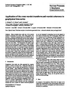
Again, increasing order of node number is used for application of this operation. The scheme followed is illustrated in Figure 1, which shows the hierarchy (constructed by the median agglomerative method, although this plays no role here), using for display convenience just the first 8 observation vectors in Fisher’s iris data [10]. We call our algorithm a Haar wavelet transform because, traditionally, this wavelet transform is defined by a similar set of averages and differences. More detailed studies of why it can with justice be called a wavelet transform can be found in [2], [24], [25], [32]. We now return to the issue of how we start this scheme, i.e. how we define s(i), or the “smooth” of a terminal node, representing a singleton cluster. We take s(i) as a vector in Rm (m-dimensional real space; which does not prejudice integer values – as in the examples below – which are of course a subset of real space), and the ith row of a data table. If our initial data matrix is denoted X, with n rows and m columns (hence each row is a point in Rm ), then we can store the detail values, d, in matrix D, and the final smooth s at hierarchy level n − 1 in such a way that:

September 28, 2005

DRAFT

APPLICATION OF THE HAAR WAVELET TREE TRANSFORM

6

X = CD + Sn−1 where D is of dimensions (n−1)×m. If sn−1 is the final data smooth, then we define Sn−1 as the n×m matrix with vector sn−1 repeated on each of the n rows. Matrix C is of dimensions n × (n − 1) and is a particular binary valued (or boolean) respresentation of the dendrogram. It is a characteristic matrix of the branching codes, where +1 and −1 are left and right branches, and 0 is a non-existent branch, with the rows being the indices of the set of observables (being clustered), and j ∈ {1, 2, . . . , n − 1} being the indices of the dendrogram levels or nodes ordered increasingly. See [32] for further background details. Constructing the hierarchical Haar wavelet transformed data is referred to as the forward transform. Reconstructing the input data is referred to as the inverse transform. The inverse transform allows exact reconstruction of the input data. We begin with sn−1 . If this root node has subnodes q and q 0 , we use d(q) and d(q 0 ) to form s(q) and s(q 0 ). We continue, step by step, until we have reconstructed all vectors associated with terminal nodes. More detail on this Haar wavelet transform of a rooted, labeled, binary tree, or dendogram, can be found in [32]. A range of experimental assessments are covered in [32], together with underlying theory.

C. Worked Example In Tables I and II we directly transform a small data set consisting of the first 8 observations in Fisher’s iris data. Note that in Table II it is entirely appropriate that at more smooth levels (i.e., as we proceed through wavelet or detail vectors, corresponding to hierarchy levels, d1, d2, . . ., d6, d7) the values become more “fractionated” (i.e., there are more values after the decimal point). The input data array shown in Table I can be exactly reproduced from the transform data shown in Table II. For this we read off, and sum, values with a “road map” provided by the binary (hierarchical clustering) tree. The minimum variance agglomeration criterion, with Euclidean distance, is used to induce the hierarchy on the given data. Each detail signal is of dimension m = 4 where m is the dimensionality of the given data. The smooth signal is of dimensionality m also. The number of detail or wavelet signal levels is given by the number of levels in the labeled, ranked hierarchy, i.e. n − 1.

III. WAVELET-BASED M ULTIWAY T REE B UILDING : A PPROXIMATING

A

H IERARCHY BY C OLLAPSING C LUSTERS A binary rooted tree, H, on n observations has precisely n − 1 levels; or H contains precisely n − 1 subsets of the set of n observations. The interpretation of a hierarchical clustering often is carried September 28, 2005

DRAFT

7

1

APPLICATION OF THE HAAR WAVELET TREE TRANSFORM

s7

+d7

-d7

s6

+d6

-d6 -d5

s5 +d5 s2 -d2

Fig. 1.

+d4

s1-d1

s3 -d3

+d3 x6

x4

x5

x3

x8

+d1 x1

x7

x2

0

+d2

s4 -d4

Dendrogram on 8 terminal nodes constructed from first 8 values of Fisher iris data. Detail or wavelet coefficients are

denoted by d, and data smooths are denoted by s.

Sepal.L

Sepal.W

Petal.L

Petal.W

1

5.1

3.5

1.4

0.2

2

4.9

3.0

1.4

0.2

3

4.7

3.2

1.3

0.2

4

4.6

3.1

1.5

0.2

5

5.0

3.6

1.4

0.2

6

5.4

3.9

1.7

0.4

7

4.6

3.4

1.4

0.3

8

5.0

3.4

1.5

0.2

TABLE I F IRST 8 OBSERVATIONS OF F ISHER ’ S IRIS DATA . L AND W REFER TO LENGTH AND WIDTH .

September 28, 2005

DRAFT

APPLICATION OF THE HAAR WAVELET TREE TRANSFORM

8

s7

d7

d6

d5

d4

d3

d2

d1

Sepal.L

5.146875

0.253125

0.13125

0.1375

−0.025

0.05 −0.025

0.05

Sepal.W

3.603125

0.296875

0.16875

−0.1375

0.125

Petal.L

1.562500

0.137500

0.02500

0.0000

0.000

−0.10

0.050

0.00

Petal.W

0.306250

0.093750

−0.01250 −0.0250

0.050

0.00

0.000

0.00

0.05 −0.075 −0.05

TABLE II T HE HIERARCHICAL H AAR WAVELET TRANSFORM RESULTING FROM USE OF THE FIRST 8 OBSERVATIONS OF F ISHER ’ S IRIS DATA SHOWN IN

TABLE I. WAVELET COEFFICIENT LEVELS ARE DENOTED D 1 THROUGH D 7, AND THE CONTINUUM OR SMOOTH COMPONENT IS DENOTED S 7.

out by cutting the tree to yield any one of the n − 1 possible partitions. Our hierarchical Haar wavelet transform affords us a neat way to approximate H using a smaller number of possible partitions. Consider the detail vector at any given level: e.g., as exemplified in Table II. Any such detail vector is associated with (i) a node of the binary tree; (ii) the level or height index of that node; and (iii) a cluster, or subset of the observation set. With the goal of “collapsing” clusters, i.e. removing clusters that are not unduly valuable for interpretation, we will impose a hard threshold on each detail vector: If the norm of the detail vector is less than a user-specified threshold, then set all values of the detail vector to zero. Other rules could be chosen, in particular rules related directly to the agglomerative clustering criterion used. We will return to this issue below to show why the norms of the detail vectors provide an excellent way to address this. Our norm-based rule is not directly related to the agglomerative criterion for the following reasons: (i) we seek a generic interpretative aid, rather than an optimal but criterion-specific rule; (ii) an optimal, criterion-specific rule would in any case be best addressed by studying the overall optimality measure rather than availing of the stepwise suboptimal hierarchical clustering; and (iii) from naturally occurring hierarchies, as occur in very high dimensional spaces (cf. [31]), the issue of an agglomerative criterion is not important. Following use of the norm-based cluster collapsing rule, the representation of the reconstructed hierarchy is straightforward: the hierarchy’s level index is adjusted so that the previous level index additionally takes the place of the given level index. Examples discussed below will exemplify this. Properties of the approach to be described include the following: 1) Rather than misleading increase in agglomerative clustering value or level, we examine instead clusters (or nodes in the hierarchy). 2) This implies that we explore a cluster at a time, rather than a partition at a time. So the resulting September 28, 2005

DRAFT

APPLICATION OF THE HAAR WAVELET TREE TRANSFORM

9

retained clusters may well come from different original partitions. 3) We take a strictly binary (2-way, agglomeratively constructed) tree as input and determine a simplified, multiway tree as output. 4) A single scalar value filtering threshold – a user-set parameter – is used to derive this output, simplified, multiway tree from the input binary tree. 5) The filtering is carried out on the wavelet-transformed tree; and then the output, simplified tree is reconstructed from the wavelet transform values. 6) The filtering is carried out on each node (in wavelet space) in sequence. Hence the computational complexity is linear. 7) Upstream of the wavelet transform, and hierarchical clustering, we use correspondence analysis to take frequency of occurrence data input, apply appropriate normalization, and map the data of interest into an (unweighted) Euclidean space. (See [33].) 8) Again upstream of the wavelet transform, for the binary tree we use minimal variance hierarchical clustering. This agglomerative criterion favors compact clusters. 9) Our hierarchical clustering accommodates weights on the input observables to be clustered. Based on the normalization used in the correspondence analysis, by design these weights here are constant.

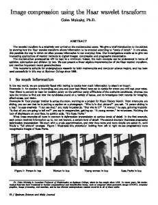
A. Properties of Derived Partition A partition by definition is a set of clusters (sets) such that none are overlapping, and their union is the global set considered. So in Figure 2 the upper left hierarchy is cut, and shown in the lower left, to yield the partition consisting of clusters (7, 8, 5, 6), (1, 2) and (3, 4). Traditionally, deriving such a partition for further exploitation is a common use of hierarchical clustering. Clearly the partition corresponds to a height or agglomeration threshold. In a multiway hierarchy, such as the one shown in the top right panel in Figure 2, consider the same straight line drawn from left to right, at approximately the same height or agglomeration threshold. It is easily seen that such a partition is the same as that represented by the non-straight curve of the lower right panel. From this illustrative example, we draw two conclusions: (i) in the case of a multiway tree a partition is furnished by a horizontal cut of the multiway tree – accomplished exactly as in the case of the strictly binary tree; and (ii) this horizontal cut of a multiway tree is identical to a nonlinear curve of the strictly binary tree. We can validly term the nonlinear curve a piecewise horizontal one. Note that the nonlinear curve used in Figure 2, lower right panel, has nothing whatsoever to do with nonlinear cluster separation (in any ambient space in which the clusters are embedded), nor with nonlinear mapping.

September 28, 2005

DRAFT

APPLICATION OF THE HAAR WAVELET TREE TRANSFORM

10

4

5

6

1

2

3

4

6

1

2

3

4

4 4

5

3 3

8

2 2

8

1 1

7

6 6

7

5 5

0 8 8

0

2

Height

4

7 7

4 2 0

Height Fig. 2.

2

Height

2 0

Height

4

0 eight 8 7 6 5 4 3 2 1 m H M

Upper left: original dendrogram. Upper right, multiway tree arising from one collapsed cluster or node. Lower left: a

partition derived from the dendrogram (see text for discussion). Lower right: corresponding partition for the multiway tree.

B. Implementation and Evaluation We took Aristotle’s Categories (see [1], [33]) in English containing 14,483 individual words. We broke up the text into 24 files, in order to study the sequential properties of the argument developed in this short philosophical work. In these 24 files, there were 1269 unique words. We selected 66 nouns of particular interest. With frequencies of occurrence in parentheses we had (sample only): man (104), contrary (72), same (71), subject (60), substance (58), species (54), knowledge (50), qualities (47), etc. Unlike in another study to be described below, no stemming or other preprocessing was applied on the grounds that singular and plurals could well indicate different semantic contenct; cf. generic “quantity”

September 28, 2005

DRAFT

APPLICATION OF THE HAAR WAVELET TREE TRANSFORM

11

versus the set of specific, particular “quantities”. (Implicit support for no stemming in the context of extensive text matching can be found in [17].) The terms × subtexts data array was doubled [33] to produce a 66 × 48 array: for each subtext j with term frequencies of occurrence aij , frequencies from a “virtual subtext” were defined as a0ij = maxij aij − aij . In this way the mass of term i, defined as proportional to the associated row sum, is constant. Thus what we have achieved is to weight all terms identically. (We note in passing that term vectors therefore cannot be of zero mass.) A correspondence analysis was carried out on the 66 × 48 table of frequencies with the aim of taking the set of 66 nouns endowed with the χ2 metric (i.e., a weighted Euclidean distance between profiles; the weighting is defined by the inverse subtext frequencies) into a factor space endowed with the (unweighted) Euclidean metric. (We note in passing that any subtexts of zero mass must be removed from the analysis beforehand; otherwise inverse subtext frequency cannot be calculated.) A hierarchical clustering (minimum variance method) was carried out on the factor coordinates of the 66 nouns. Such a hierarchical clustering is a strictly binary (i.e. 2-way), rooted tree. The norms of detail vectors had minimum, median and maximum values as follows: 0.0758, 0.2440 and 0.6326, and these influenced the choice of threshold. Applying thresholds of 0, 0.2, 0.3 and 0.4 gave rise to the following numbers of “collapsed” clusters with, in brackets, the mean squared error between approximated data and original input data: 0 (0.0), 23 (0.0054), 44 (0.0147), and 55 (0.0164). Figure 3 shows the corresponding reconstructed and approximated hierarchies. In the case of the threshold 0.3 (lower left in Figure 3) we have noted that 44 clusters were collapsed, leaving just 21 partitions. As stated the objective here is precisely to approximate the dendrogram output data structure in order to facilitate further study and interpretation of these partitions. Figure 4 shows the sequence of agglomerative levels where each panel corresponds to the respective panel in Figure 3. It is clear here why these agglomerative levels are very problematic if used for choosing a good partition: they increase with agglomeration, simply because the cluster centers are getting more and more spread out as the sequence of agglomerations proceeds. Directly using these agglomerative levels has been a way to derive a partition for a very long time. An early reference is [26]. To see how the detail norms used by us here are different, see Figure 5.

C. Collapsing Clusters Based on Detail Norms: Evaluation Vis-`a-vis Direct Partitioning Our cluster collapsing algorithm is: wavelet-transform the hierarchical clustering; for clusters corresponding to detail norm less than a set threshold, set the detail norm to zero, and the corresponding increase in level in the hierarchy also; reconstruct the hierarchy. We look at a range of threshold values. To begin with, the hierarchical clustering is strictly binary. Reconstructed hierarchies are multiway.

September 28, 2005

DRAFT

APPLICATION OF THE HAAR WAVELET TREE TRANSFORM

12

Fig. 3.

0.04 0.02 0.0020 0.0000

0.00

0.003 0.000

0.00

0.02

0.04

0.00 0.02 0.01 0.04 0.03 0.000 0.003 0.002 0.001 m 0.005 0.004 0.0000 0 0.0020 0.0015 0.0010 0.0005 M 0.0030 0.0025 .00 .02 .04 .000 .003 .0000 .0020

Upper left: original hierarchy. Upper right, lower left, and lower right show increasing approximations to the original

hierarchy based on the “cluster collapsing” approach described.

For each unique level of such a multiway hierarchy (cf. Figure 3) how good are the partitions relative to a direct, optimization-based alternative? We use the algorithm of Hartigan and Wong [16] with a requested number of clusters in the partition given by the same number of clusters in the collapsed cluster multiway hierarchy. In regard to the latter, we look at all unique partitions. (In regard to initialization and convergence criteria, the Hartigan and Wong algorithm implementation in the R package, www.r-project.org, was used.) P We characterize partitions using the average cluster variance, 1/|Q| i∈q;q∈Q 1/|q|ki − qk2 . AlP ternatively we assessed the sum of squares: q∈Q ki − qk2 . Here, Q is partition, q is a cluster, and

September 28, 2005

DRAFT

APPLICATION OF THE HAAR WAVELET TREE TRANSFORM

13

0.04 0.00

0.02

Height

0.02 0.00

Height

0.04

0.00 0.02 0.01 0.04 0.03 0.001 0.004 0.003 0.002 0.005 1 10 3 30 20 5 50 40 m 60 0.0005 0 0.0020 0.0015 0.0010 Levels 0.0030 0.0025 L H M Height .00 .02 .04 .001 .004 0 .0005 .0020 evels eight 1 to 65

0 10

30

50

0 10

0.0020 0.0005

0 10

30

50

Levels 1 to 65

Fig. 4.

50

Levels 1 to 65

Height

0.004 0.001

Height

Levels 1 to 65

30

0 10

30

50

Levels 1 to 65

Agglomerative clustering levels (or heights) for each of the hierarchies shown in Figure 3.

ki − qk2 is Euclidean distance squared between a vector i and its cluster center q. (Note that q refers both to a set and to a cluster center – a vector – here.) Although this is a sum of squares criterion, as Sp¨ath ([36], p. 17) indicates, it is on occasion (confusingly) termed the variance criterion. In either case, we target compact clusters with this k-means clustering algorithm, which is also the target of our hierarchical agglomerative clustering algorithm. A k-means algorithm aims to optimize the criterion, in the Sp¨ath sense, directly. In Table III-C we see that the partitions of our multiway hierarchy are about half as good as kmeans in terms of overall compactness (cf. columns 3 and 5). Close inspection of properties of clusters in different partitions indicated why this was so: with a poor or low compactness for one cluster very

September 28, 2005

DRAFT

APPLICATION OF THE HAAR WAVELET TREE TRANSFORM

14

0.5 0.1

0.3

Height

0.02 0.00

Height

0.04

0.00 0.02 0.01 0.04 0.03 1 10 3 30 20 5 50 40 m 60 0.1 0.3 0.2 0 0.5 0.4 Levels 0.6 L H M Height .00 .02 .04 0 .1 .3 .5 evels eight 1 to 65

0 10

30

50

0 10

Levels 1 to 65

Fig. 5.

30

50

Levels 1 to 65

Agglomerative levels (left; as upper left in Figure 4, and corresponding to the original – upper left – hierarchy shown

in Figure 3), and detail norms (right), for the hierarchy used. Detail norms are used by us as the basis for “collapsing clusters”.

early on in the agglomerative sequence, the stepwise algorithm used by the multiway hierarchy had to live with this cluster through all later agglomerations; and the biggest sized cluster (i.e. largest cluster cardinality) in the stepwise agglomerative tended to be a little bigger than the biggest sized cluster in the k-means result. This is an acceptable result: after all, k-means optimizes this criterion directly. Furthermore, the multiway hierarchy preserves embededness relationships which are not necessarily present in any sequence of results ensuing from a k-means algorithm. Finally, it is well-known that seeking to directly optimize a criterion such as k-means will lead to a better outcome than the stepwise refinement used in the stepwise agglomerative algorithm. If we ask whether k-means can be applied once, and then k-means applied to individual clusters in a recursive way, the answer is of course affirmative – subject to prior knowledge of the number of levels and the value of k throughout. It is precisely in such areas that our hierarchical approach is to be preferred: we require less prior knowledge of our data, and we are satisfied with the downside of global approximate fidelity between output structure and our data. In the study of automatic query term expansion, below, we will approach the comparative assessment vis-`a-vis k-means differently: we will look for a 20-cluster partition in the original hierarchy (i.e., 20 levels from the root), and in k-means, but in the case of the multiway tree we will use the partition which is 20 levels from the top – associated with a greater number of clusters. When we do this, we have a better chance of outscoring k-means. This we will see below (in section V).

September 28, 2005

DRAFT

APPLICATION OF THE HAAR WAVELET TREE TRANSFORM

15

Agglom. Multiway tree Multiway tree

Partition

K-means

level

height

partition SS cardinality partition SS

1

0.00034

0.095

65

0.062

2

0.00042

0.229

61

0.091

3

0.00051

0.340

60

0.146

4

0.00057

0.397

59

0.205

5

0.00059

0.485

58

0.156

6

0.00066

0.739

55

0.239

7

0.00077

1.115

53

0.347

8

0.00092

1.447

51

0.484

9

0.00099

1.723

48

0.582

10

0.00122

2.329

45

0.852

11

0.00142

2.684

43

0.762

12

0.00159

3.101

42

0.865

13

0.00161

3.498

39

1.161

14

0.00189

3.938

36

1.354

15

0.00201

4.954

32

1.873

16

0.00220

5.293

30

2.178

17

0.00234

6.957

25

3.007

18

0.00311

7.204

24

2.722

19

0.00314

8.627

21

3.497

20

0.00326

10.192

15

5.426

21

0.00537

18.287

1

18.287

TABLE III A NALYSIS OF THE UNIQUE PARTITIONS IN THE MULTIWAY TREE SHOWN ON THE LOWER LEFT OF F IGURE 3. PARTITIONS ARE BENCHMARKED USING K - MEANS TO CONSTRUCT PARTITIONS WHERE K IS THE SAME VALUE AS FOUND IN THE MULTIWAY TREE .

SS = SUM OF SQUARES CRITERION VALUE .

IV. A PPLICATION TO C ONCEPT H IERARCHY C ONSTRUCTION A. Motivation Our wavelet-based multiway tree building approach provides a scalable (computational complexity of polynomial order 2), data-driven algorithm requiring more limited user parameter setting compared to previous work. Similarly to [8], [9] we require a “broad and shallow multiway tree representation” of our data, rather than a “narrow and deep binary tree”, and this we do with (i) an integrated algorithm, and (ii) with one thresholding parameter to be fixed by the user (instead of a number of user parameters to be set or fixed by the user in [9], section 3.2).

September 28, 2005

DRAFT

APPLICATION OF THE HAAR WAVELET TREE TRANSFORM

16

Other approaches include “weakly supervised hierarchical clustering” [4], or “guided” hierarchical agglomerative clustering [6]. Approaches based on Kohonen’s self-organizing feature map have been studied in [22], [23]. A lattice, rather than a tree, approach has also been pursued by some authors [14], [7].

B. Case Study In order to have a flat multiway hiearchy we took our Categories data (see section III-B) and applied a (very restrictive) wavelet filtering threshold of 0.55, which led to just two levels in the resultant, reconstruced multiway hierarchy. In the latter there are 10 non-singleton clusters with cardinalities of: 2, 2, 14, 2, 3, 2, 2, 2, 2, 6. These clusters associated the following terms, respectively: 1) name existence 2) definition object 3) substances boundary category habit alteration genera proposition cubits differentiae disease instances justice mark number 4) quantity socrates 5) sight nature blind 6) fact disposition 7) position motion 8) variation blindness 9) statement sort 10) capacity correlatives master affections quantities class Note how both terms quantity and quantities appear here because we did not using stemming. We take the view here that quite often there is semantic difference between singular and plural. We recall that Aristotelian technical terms, as used in the Categories, were taken from erstwhile regular, colloquial speech. This lends support to the bottom-up process that we are using to determine a meaningful concept hierarchy, as opposed to the top-down, a priori approach that starts with a restricted technical vocabulary. We do not have a methodology for labeling such clusters. In some cases, the clusters seem very reasonable and we could well find an appropriate label (e.g. in the cases of clusters 1, 2, 5, 6, 7, 8). For the others (clusters 3, 4, 9, 10) we would need to look closer at our data, to understand them (in particular the tighter, smaller clusters 4 and 9). An alternative of course could be to redo the entire analysis without such terms as socrates justice master, etc. Because relative relationships will change (subtexts may be dropped, lots of terms will disappear) the clustering properties will necessarily change.

September 28, 2005

DRAFT

APPLICATION OF THE HAAR WAVELET TREE TRANSFORM

17

We did just this for the terms in clusters 1, 2, 6 and 7 above. Figure 6 shows the result. We can now more easily label the clusters. Let us do so: state = {motion, position}; thing = {object, state}; character = {disposition, thing}; characteristic = {existence, fact}; label = {name, definition}; characterization = {characteristic, thing}, labeled character = set of all terms = {label, characterization}. Our aim here is to show clearly the mechanism which allows a concept hierarchy to be built in a bottom-up, data-driven way. From our initial, large hierarchical clustering, containing extraneous and irrelevant detail, we used wavelet filtering to produce a more cogent “guess” of the desired concept hierarchy. This wavelet filtering required use of a filtering threshold – one single scalar value. Then, through user interaction, a more appropriate set of terms was selected. Finally cluster labeling or characterization is carried out by the user or domain specialist.

V. A PPLICATION TO AUTOMATIC T ERM E XPANSION A. Motivation The cluster collapsing objective was motivated by the need for a practical approach to concept hierarchy construction, for use in term expansion [20] in a free-text query and answer system. Our prototype was implemented as a servlet with parallel English and Spanish language versions.

B. Implementation We take a set of 34 texts crossed by 392 terms. The former are Q&A texts from a web-based FAQ on effects on health of electromagnetic radiation (from cellphone masts etc.): see [27]. The latter are Porter-stemmed [34] terms that are in the middle region (determined by user-fixed thresholds) of the Zipf rank-frequency chart. Examples of the latter: field studi exposur power cancer frequenc report magnet electr Normalization (by row or column or both) is of great importance. Firstly we used the correspondence analysis (row-wise) doubling of the data matrix, A, to produce a new input matrix which, when transposed, was of dimensions 392×68. For typical term j and text i, the given frequency of occurrence was aji , and in doubling (see subsection III-B) we created an additional new value, a0ji , defined as maxij aij − aji . Therefore the marginal distribution of the 392 terms, defining their masses for use in correspondence analysis – and in the hierarchical clustering to follow later – are identical. Correspondence analysis results in an output factor space dimensionality of the minimum of 34 and 392. Without loss of generality we will retain 30 factors. Hierarchical clustering with the minimum variance (also known as Ward’s) method, with constant weighting, is applied to the 392 terms, each characterized by projections on the 30 factors. This gives a dendrogram or hierarchical clustering on the 392 terms. September 28, 2005

DRAFT

APPLICATION OF THE HAAR WAVELET TREE TRANSFORM

18

position

motion

object

disposition

fact

existence

definition

name

0.04 0.00

Height

0.08

0.12

nact definition e fexistence fact d disposition o object motion p position m 0.00 0.04 0.02 0.08 0.06 0 0.12 0.10 H Height 0.14 M ame efinition xistence isposition bject osition .00 .04 .08 .12 eight otion

Fig. 6. A hierarchy using just 8 terms crossed by 23 subtexts of Aristotle’s Categories for specification of a concept hierarchy.

Dendrogram Haar a` trous wavelet filtering is applied as follows. We determine the norm of each detail vector, and (knowing the maximum, medium and minimum norm values) apply a hard threshold. If the norm is below the threshold then the dendrogram increase in level of that detail vector is set to zero; and we set the associated detail coefficients to zero. We applied Haar dendrogram thresholds of 0.03, 0.05 and 0.07 to yield increasingly “collapsed” clustering hierarchies. (These corresponded to the collapsing of 62, 194 and 269 clusters; and to MSE discrepancy between input and outputs: 8e−5, 0.00025, 0.00057 respectively.) We then characterized the clusters in the reconstructed hierachy. Since a level of the hierarchy implies a precise number of clusters, the best case for us is when the 392 terms are evenly divided

September 28, 2005

DRAFT

APPLICATION OF THE HAAR WAVELET TREE TRANSFORM

19

20 4 40 6 60 8 80 100 1 10000 0 m 2 20000 3 30000 Dendrogram D MSE MSE M M 0endrogram 00 0000 SE SE of partitions level from (from root root) (1 = root)

20000 0

10000

MSE

30000

MSE of partitions (from root)

0

20

40

60

80

100

Dendrogram level from root (1 = root)

Fig. 7.

Rightmost curve: MSEs from original hierarchy. Curves in sequence from upper right to lower left: MSEs from

increasingly approximated reconstructions of the original hierarchy based on the “cluster collapsing” approach described.

between these clusters. An overall definition of diversity from this ideal case is by means of the mean square error of cluster cardinalities. Figure 7 shows the MSE curves for the original dendrogram, the 0.3-, the 0.5-, and the 0.7-thresholded dendrograms, respectively from upper right to lower left. There are 391 levels in the dendrogram (viz., 392 − 1) and we show for clarity the top 100 levels (from left to right in Figure 7). Dendrogram level 1, where all terms are in the same cluster, has an MSE value of 0. Dendrogram level 2 is quite imbalanced in cluster cardinality, resulting in the high MSE value. We see that the greater the wavelet filtering, the greater the balance in the hierarchy partitions. Looking at the individual clusters, we ask if the partition derived from the filtered (“collapsed”) hierarchy can be shown to be better than (i) an analogous partition derived directly (with no wavelet filtering) in the traditional way from the hierarchy, or (ii) an alternative partition based on k-means clustering (i.e., based on direct iterative optimization of a sum of cluster compactness values). With reference to Figure 7 we choose the partition with 20 clusters in the original hierarchy; the partition with 20 clusters in k-means; and for the filtered or “collapsed” hierarchy, we take the 20th level from the root, i.e. the same 20th level from the root as used for the original hierarchy. The latter corresponds to a much greater number of clusters in the case of the multiway or “collapsed” tree. In general terms we find the following. The original hierarchy gives a partition with very few, very

September 28, 2005

DRAFT

APPLICATION OF THE HAAR WAVELET TREE TRANSFORM

20

Orig. O dataset0 250 200 K-means, 350 300 K dataset1 15 Multiway M d dataset2 F Frequency 2 20 10 4 40 30 6 60 5 50 0 m 70 1 100 M 150 ataset0 ataset1 5 50 ataset2 0 00 requency -means, rig. ultiway 20-clus. hier., 20-clus. part. 20 levs. part. < root

150

Frequency

K-means, 20-clus. part.

0

50

250 100 0

Frequency

Orig. 20-clus. part.

0

5

10

15

20

dataset0

0

5

10

15

20

dataset1

100 50 0

Frequency

Multiway hier., 20 levs. < root

0

20

40

60

dataset2

Fig. 8.

Histograms of cluster sizes (cardinalities) in orgininal data (upper left), k-means (upper right), and the partition from

the multiway hierarchy (lower left). See text for further details.

large clusters, and many singleton clusters. The filtered/“collapsed” hierarchy tends to break up – to some extent – the very large clusters and to leave untouched the singleton clusters. Finally k-means removes most if not all singletons, but the thought arises as to how compact the resulting clusters are. For 392 terms, with the original hierarchy, we find a very big cluster of 346 terms, and just 5 other non-singleton clusters; and the largest cluster variance (for a cluster with 9 members, not the very big 346-member one) was 0.237. For the k-means clustering, all 20 cluster sizes were small – given the direct, iterative compactness optimization – but the largest cluster variance for a cluster with just 4 members was 0.134 (a high value, relative to cluster variances with far greater cardinalities). This confirms our belief that k-means will give a balanced spread of clusters sizes, but at the expense of perhaps unjustifiably large variance clusters. Finally, the filtered or “collapsed” partition had maximum cluster size 149, and (for a different small-sized cluster) maximum variance 0.228. Figures 8 summarizes these results: a 20-cluster partition of the original hierarchy is used; a 20cluster partitition furnished by k-means; and a 69-cluster partition, at 20 levels form the root, in the multiway tree yielded by the 0.07 filtering threshold value. We see greater relative balance of cluster cardinalities in the last of these, viz., the partition derived from the multiway hierarchy. We must note how we define variance: using the cluster labels, the data used in all cases are the

September 28, 2005

DRAFT

APPLICATION OF THE HAAR WAVELET TREE TRANSFORM

21

factor projections, i.e. the inputs to the hierarchical and k-means algorithms. To characterize the overall partition, we looked at the sum of variances of all clusters, averaged by the number of non-singleton clusters. For the original hierarchy partition, this was 0.086. For k-means, it was 0.047. Finally, for the filtered hierarchy partition, it was 0.036. This last favorable result presents evidence for the filtered partition as being the best from a practical viewpoint. It also supports the visual evidence of Figure 8. In sum, the arguments presented in this subsection in favor of our cluster “collapsing”, tree filtering algorithm are (i) superior effectiveness under appropriate circumstances; and (ii) these appropriate circumstances are additionally motivated by limited or weak user parameter inputs (respectively, the threshold in the wavelet filtering; and the choice of level to cut the multiway tree).

C. Relative Recall and Precision Analysis of recall and precision of a partition derived from our cluster collapsing, or tree waveletbased, algorithm requires ground truth data. However relative recall and precision can be addressed more easily. Our baseline is to look at each term retained in our system, and the text which is most associated with each term. Exhaustive querying of the text collection is feasible whenever the total number of terms in our controlled vocabularly is not large: here it is 392. Next we take the partition derived from the wavelet-processed hierarchy. We exclude overly large clusters from consideration. This capping is set at a cluster cardinality of 9 terms. Apart from singleton clusters we are also left then with clusters of cardinalities: 3, 6, 5, 3, 5, 2, 5, 2, 3, 4, 4, 2, 7, 2, 3, and 2. For singleton clusters, the performance under any circumstances is identical between benchmark case and the partition/term expanion case. For clusters of overly large cardinality, we use singletons and again performance is identical. For retained, non-singleton clusters (cardinalities listed above), we look at (i) the nearest neighbor text of each cluster member, and (ii) the ranked lists of texts retrieved by the cluster. Closeness is defined as scalar product, i.e. sum of shared terms, weighted by frequency of terms in the cluster. This is a simple voting measure, using frequency of occurrence. Note that the similarity (or dissimilarity) used is not crucial because we just want an adequate measure here in order to study comparable query performance in a relative way. We find that taking the list of top ranked 4-nearest neighbor texts of each cluster is sufficient to have included among these 4-nearest neighbors the 1-nearest neighbor text of each of the constituent terms in the cluster. Through use of 4-nearest neighbors in the term expansion case, there is no difference in performance

September 28, 2005

DRAFT

APPLICATION OF THE HAAR WAVELET TREE TRANSFORM

22

over 1-nearest neighbors in the benchmark case (with no term expansion). This result holds for the particular data used, the wavelet-based partition used, and querying using each term individually. Relative to the benchmark (i.e., nearest neighbor or best match) case, we see that there is no difference in system performance. What clustering offers is (i) implicit collaborative filtering in that terms are used in addition to the user-provided terms, and (ii) potential computation improvement in that an inverted clusters-to-texts mapping replaces the inverted terms-to-texts mapping.

VI. C ONCLUSIONS An innovative methodology has been described, for wavelet transforming a tree. The transform and its inverse have been developed for a binary, rooted, labeled tree which represents an agglomerative, hierarchical clustering. Tree filtering, or tree approximation, can be facilitated greatly by processing the wavelet-transformed data, and then applying the inverse transform. We have discussed the advantages of (and lack of feasible alternatives for) approximating a tree in this way. We then showed how tree approximation can be used to derive in a semi-automatic way a better hierarchy for use as an ontology or concept hierarchy. In a further case study we showed how tree approximation permits a better partition to be derived – better in the sense of taking clusters into account at various levels of the initially given binary tree. The application used in this case study, which has been implemented as a web-accessible servlet demonstrator, is that of query expansion in best match based information retrieval.

ACKNOWLEDGEMENTS Dimitri Zervas and Pedro Contreras contributed to the coding, and to implementation of the query term expansion demonstrator.

R EFERENCES [1] Aristotle, The Categories, 350 BC. Translated by E.M. Edghill. Project Gutenberg e-text, www.gutenberg.net [2] J.J. Benedetto and R.L. Benedetto, “A Wavelet Theory for Local Groups and Related Groups”, The Journal of Geometric Analysis, vol. 14, pp. 423–456, 2004. [3] J.P. Benz´ecri, La Taxinomie, 2nd ed., Dunod, 1979. [4] P. Buitelaar, P. Cimiano and B. Magnini, Eds., Ontology Learning from Text: Methods, Evaluation and Applications, IOS Press, 2005. [5] K. Chakrabarti, M. Garofalakis, R. Rastogi, and K. Shim, “Approximate Query Processing using Wavelets”, VLDB Journal, International Journal on Very Large Databases, vol. 10, pp. 199–223, 2001. [6] P. Cimiano and S. Staab, “Learning Concept Hierarchies from Text with a Guided Agglomerative Clustering Algorithm”, Proceedings of the ICML 2005 Workshop on Learning and Extending Lexical Ontologies with Machine Learning Methods, 2005. September 28, 2005

DRAFT

APPLICATION OF THE HAAR WAVELET TREE TRANSFORM

23

[7] P. Cimiano, A. Hotho and S. Staab, “Learning Concept Hierarchies from Text Corpora Using Formal Concept Analysis”, Journal of Artificial Intelligence Research, 24, 2005, in press. [8] Shui-Lung Chuang and Lee-Feng Chien, “Automatic Query Taxomomy Generation for Information Retrieval Applications”, Online Information Review, vol. 27, pp. 243–255, 2003. [9] Shui-Lung Chuang and Lee-Feng Chien, “Topic Hierarchy Generation for Text Patters: A Practical Web-Based Approach”, ACM Transactions on Information Systems, in press, 2005. [10] R.A. Fisher, “The Use of Multiple Measurements in Taxonomic Problems”, The Annals of Eugenics, vol. 7, pp. 179–188, 1936. [11] R. Foote, “An Algebraic Approach to Multiresolution Analysis”, Transactions of the American Mathematical Society, 357, 5031–5050, 2005. [12] M.W. Frazier, An Introduction to Wavelets through Linear Algebra, Springer, 1999. [13] A. G´omez-P´erez, M. Fern´andez-L´opez and O. Corcho, Ontological Engineering (with Examples from the Areas of Knowledge Management, e-Commerce and the Semantic Web), Springer, 2004. [14] H.-M. Haav, “An Application of Inductive Concept Analysis to Construction of Domain-Specific Ontologies”, VLDB, 2003. [15] W. H¨ardle, Wavelets, Approximation, and Statistical Applications, Springer, 2000. [16] J.A. Hartigan and Wong, M.A., “A K-means Clustering Algorithm”, Applied Statistics, 28, 100-108, 1979. [17] D.A. Hull, “Stemming Algorithms: A Case Study for Detailed Evaluation”, Journal of the American Society for Information Science, vol. 47, pp. 70–84, 1996. [18] M.J. Joe, K.-Y. Whang, and S.-W. Kim, “Wavelet Transformation-Based Management of Integrated Summary Data for Distributed Query Processing”, Data and Knowledge Engineering, vol. 39, pp. 293–312, 2001. [19] S.C. Johnson, “Hierarchical Clustering Schemes”, Psychometrika, vol. 32, pp. 241–254, 1967. [20] K. Sparck Jones, Automatic Keyword Classification for Information Retrieval, Butterworths, London, 1971. [21] H. Kargupta and B.-H. Park, “A Fourier Spectrum-Based Approach to Represent Decision Trees for Mining Data Streams in Mobile Environments”, IEEE Transactions on Knowledge and Data Engineering, vol. 16, pp. 216–229, 2004. [22] Latifur Khan and Feng Luo, “Ontology Construction for Information Selection”, Proc. IEEE International Conference on Tools with Artificial Intelligence, ICTAI’02, pp. 122–127, 2002. [23] L. Khan and L. Wang, “Automatic Ontology Derivation using Clustering for Image Classification”, in Proc. of Eighth International Workshop on Multimedia Information Systems, pp. 56–65, 2002. [24] S.V. Kozyrev, “Wavelet Theory as p-Adic Spectral Analysis”, Izvestiya: Mathematics, vol. 66, pp. 367–376, 2002. [25] S.V. Kozyrev, “p-Adic Pseudodifferential Operators and p-Adic Wavelets”, Theoretical and Mathematical Physics, vol. 138, pp. 322–332, 2004. [26] R. Mojena, “Hierarchical grouping methods and stopping rules: an evaluation”, The Computer Journal, vol. 20, pp. 359–363, 1977. [27] J.E. Moulder, “Electromagnetic Fields and Human Health – Power Lines and Cancer FAQs”, www.mcw.edu/gcrc/cop/powerlines-cancer-FAQ/toc.html (last updated 2005-7-11), 2005. [28] F. Murtagh, Multidimensional Clustering Algorithms, Physica-Verlag, 1985.

September 28, 2005

DRAFT

APPLICATION OF THE HAAR WAVELET TREE TRANSFORM

24

[29] F. Murtagh, “Wedding the Wavelet Transform and Multivariate Data Analysis”, Journal of Classification, vol. 15, pp. 161–183, 1998. [30] F. Murtagh, J.-L. Starck, and M. Berry, “Overcoming the Curse of Dimensionality in Clustering by Means of the Wavelet Transform”, The Computer Journal, vol. 43, pp. 107–120, 2000. [31] F. Murtagh, “On Ultrametricity, Data Coding, and Computation”, Journal of Classification, vol. 21, pp. 167– 184, 2004. [32] F. Murtagh, “The Haar Wavelet Transform of a Dendrogram – I, – II” submitted, 2005. (Copy at: www.cs.rhul.ac.uk/home/fionn/papers) [33] F. Murtagh, Correspondence Analysis and Data Coding with Java and R, Chapman and Hall/CRC Press, 2005. [34] M.F. Porter, “An Algorithm for Suffix Stripping”, Program, vol. 14, pp. 130–137, 1980. (Code at www.tartarus.org/∼martin/PorterStemmer) [35] R. Rammal, G. Toulouse, and M.A. Virasoro, “Ultrametricity for Physicists”, Reviews of Modern Physics, vol. 58, pp. 765–788, 1986. [36] H. Sp¨ath, Cluster Dissection and Analysis, Ellis Horwood, 1985. [37] J.-L. Starck and F. Murtagh, Astronomical Image and Data Analysis, Springer, 2002. Chapter 9: “Multiple Resolution in Data Storage and Retrieval”. [38] G. Strang and T. Nguyen, Wavelets and Filter Banks, Wellesley-Cambridge Press, 1996. [39] Tao Li, Qi Li, Shenghuo Zhu, and Mitsunori Ogihara, “A Survey on Wavelet Applications in Data Mining”, SIGKDD Explorations, vol. 4, pp. 49–68, 2002. [40] J.S. Vitter and M. Wang, “Approximate Computation of Multidimensional Aggregates of Sparse Data using Wavelets”, in Proceedings of the ACM SIGMOD International Conference on Management of Data, pp. 193–204, 1999.

September 28, 2005

DRAFT