EIT images of the solar corona [29], that is, the ones we are going to discuss in ... ization to the wavelet setup of the familiar Fourier power spectrum.1 In the ...
APPLICATION OF THE 2-D WAVELET TRANSFORM TO ASTROPHYSICAL IMAGES
J-P. Antoine1 , L. Demanet1 , J-F. Hochedez2 , L. Jacques1 , R. Terrier3 , and E. Verwichte2 1
2
3
Institut de Physique Th´eorique, Universit´e Catholique de Louvain B-1348 LOUVAIN-LA-NEUVE (Belgium) Solar Departement, Royal Observatory of Belgium B-1080 BRUSSELS (Belgium) Service d’Astrophysique, CEA Saclay F-91191 GIF-SUR-YVETTE (France) Abstract
The 2-D continuous wavelet transform has been applied to a number of problems in astrophysics. We survey quickly some of these, then focus on two new applications. The first one is the automatic detection and analysis of special objects from the solar corona in the data taken by the EIT instrument aboard the SoHO satellite. The second problem is the detection of gamma sources in the Universe, the difficulty lying in the discrimination of faint sources against a highly nonuniform background and the large number of sources (to be) measured by satellites like EGRET and GLAST.
1
Introduction
The wavelet transform has become a standard tool in signal and image processing, and it has found applications to almost all fields of physics, engineering and applied mathematics. In this paper, we will focus on its applications to astronomy and astrophysics imagery. This means that we will consider the two-dimensional version of the transform and, more precisely, the 2-D continuous wavelet transform (CWT). Its main use is for analysis and feature detection in images, with special emphasis on the detection of singularities (contours, sharp transitions, etc.). By contrast, the discrete WT is more appropriate for signal compression and reconstruction, and it is the most popular version in the signal processing community. For the convenience of the reader, we recall in the Appendix the basic facts about the 2-D CWT. Further information may be found in the original paper [1], in review articles such as [2] or [4], or in a the standard textbook like [14].
1
2
Applications of the 2-D wavelet transform in astronomical imaging
The wavelet transform has been applied to many different problems in astronomy and astrophysics, both in 1-D and in 2-D. We will quickly review some of them, concentrating on the latter, that is, application of the CWT to astronomical/astrophysical images. The first attempt to apply the CWT for astrophysical images is due to the group of A. Bijaoui in Nice, in 1990. In their pioneering paper [32], they used the CWT for the analysis of galaxy clusters. The rationale for choosing the CWT is the following. First, many astrophysical objects are variable (an extreme example is that of gamma ray bursts!), which points towards a time-frequency method. Next, the Universe has a distinctly hierarchical structure: stars, galaxies, galaxy clusters and superclusters correspond to different scales (i.e., sizes), so that a time-scale analysis is better adapted. In other words, wavelet analysis is a suitable tool. Now, the main problem is that of detecting particular features, relations, groupings, etc, in images, which leads to prefer the continuous WT over the discrete WT. Finally, there is in general no privileged direction, nor particular oriented features in astrophysical images. All this suggests to use the simplest isotropic 2-D wavelet, namely the 2-D Mexican hat. This was proposed in [32], and followed by almost all later papers. In the two papers [32, 33], the authors exploited galaxy counts to identify both galaxy clusters and voids, pointing to a possible fractal structure. This led them to the analysis of the large scale structure of the Universe, for which they developed a multiscale vision model [8, 7] in order to detect and to characterize structures of different sizes (for numerical reasons, also linked to the necessity of denoising the images, they later switched to a discrete WT, based on spline wavelets). For instance, they proposed in [25] a morphological indicator allowing a comparison between various cosmological models (for instance, cold vs. hot dark matter). They have even applied their vision model to the analysis of EIT images of the solar corona [29], that is, the ones we are going to discuss in Section 3. Another topic where the CWT has been applied successfully is the analysis of the X-ray structure of various objects, such as clusters of galaxies, following a suggestion by Grebenev et al. [20]. This leads to a different class of problems. Indeed, such sources are frequently at the limit of detection, so that statistical considerations become crucial. In particular, we are here often in the photon-counting regime, the photon per pixel statistics is significantly different from Gaussian and most sources are extended. The analysis of such images by wavelet methods was further developed by Damiani et al. [13]. Our own work reported in Section 4 uses a similar approach, but goes significantly deeper in the analysis. In particular, considerable care will be devoted to the presence of Poisson noise in the photon flux (note a recent attempt in the same direction by Bijaoui and Jammal [10]). A third research area where the CWT has been used is the detailed analysis of individual galaxies, notably in the group of P. Frick in Perm, Russia [17]. Of particular importance is the cross-correlation between images obtained at different wavelengths. In [18], the authors introduce the notion of wavelet spectrum, which is the proper general-
2
ization to the wavelet setup of the familiar Fourier power spectrum.1 In the same vein, the authors of [18] advocate the use of the wavelet cross-correlation function for comparing the CWTs of their different images. Note that in their treatment they use both the Mexican hat wavelet and, for a better separation of scales, their own isotropic wavelet, defined in (A.13). This wavelet may have an independent interest. Finally, a group from Santander, Spain, has undertaken a systematic analysis, by wavelet methods, of the COBE data on the cosmic microwave bakground (CMB) radiation. In a first step, they studied the local (i.e., in small sky patches) temperature anisotropies in the CMB, including denoising the images, using both Haar and Mexican hat wavelets (not necessarily isotropic) [30, 31]. Later [11], they used the isotropic Mexican hat to detect and determine the flux of point sources superimposed on the CMB, in conditions simulating the Planck Surveyor mission. As they point out, and we will have more to say on that later, the advantage of the wavelet method is that no assumption has to be made regarding the statistical properties of the point source population or the underlying emission of the CMB. They showed that the isotropic Mexican hat wavelet is in fact optimal for detecting point sources, and they also made a detailed comparison of the wavelet method with the standard maximum-entropy method [37]. Their conclusion is that the two methods are in fact complementary and can be combined to improve the accuracy of the detection. Then, more recently, the Santander group turned to a global analysis of the CMB, trying to detect potential non-Gaussian CMB temperature fluctuations. This is an important observation for cosmology, for any non-Gaussianity would be an evidence for a departure from standard inflationary theories. Since the data used in these experiments is the full sky COBE-DMR data, it is clear that the sphericity of the data has to be taken into account. As a consequence, one has to resort to spherical wavelets. A first attempt was made by Barreiro et al. [6], using spherical Haar wavelets. Then the Santander group introduced the spherical Mexican hat, establishing the superior capability of the latter over the Haar wavelets [26]. The net result of these investigations is that the CMB temperature fluctuations [12] are consistent with a Gaussian distribution, thus vindicating the standard theories. All these papers, and many more we have not quoted, prove that the CWT, both Euclidean and spherical, is a powerful tool in the analysis of astrophysical images. The two new applications presented here will be an eloquent confirmation of that statement.
3
Application of the CWT in Solar astronomy
Since 1996, the Extreme-ultraviolet Imaging Telescope (EIT) on board the Solar and Heliospheric Observatory (SoHO) satellite observes the Sun in four wavelengths: 171 ˚ A, ˚ ˚ ˚ 195 A, 284 A and 304 A (see Figure 1). These correspond respectively to particular emission lines of Iron (IX-X, XII, XV) and Helium (II), and thus to special temperatures which are typical of those of the Sun Corona in the first three wavelengths, and of the Transition Region in the fourth one [15]. � This quantity, which is defined as M (a) = R2 d2�b |WI (�b, a)|2 , was also introduced by some of us [3] in a totally different context (detection of symmetries in 2-D patterns.) 1
3
304 ˚ A (red)
171 ˚ A (blue)
195 ˚ A (green)
274 ˚ A (yellow)
Figure 1: Images of the Sun in the four recorded wavelengths of EIT 3.1
The problem
The Sun Corona is physically very complex and contains a huge amount of different events appearing at different location and scales. Solar astronomers are interested in the physics which can be deduced from them to improve our knowledge of the global Sun. One way to achieve this is to make time statistics on features of special solar objects.2 Because of the large number of EIT pictures (currently greater than 100 000), astronomers aim also to realize this analysis automatically by some well-suited algorithms. However, many conceptual problems arise due to the difference between the human description of things and the true (logical) computer vision. These can be summarized into two main questions: • How to define a Sun corona object in simple terms, that is, in sufficiently simple concepts which can be managed by a computer program? 2
This follows the discovery of the 11 year solar cycle by the periodicity in time of the latitude of the sunspots.
4
• How to determine the relevant characteristics of such an object and how to translate them as simply as possible? After a short description of the common Sun corona objects, we will show that the continuous wavelet transform (CWT) offers tools to answer these fundamental questions. 3.2
Special coronal objects
The physical objects of the Sun corona result in general from convective motions in the solar mantle and/or of magnetic interactions with hot material. Here is a list of the principal objects, ordered by size, from the smallest to the largest (for more information see [22, 15, 28]): ˚ images, the magnetic network constitutes a texMagnetic network: In the red 304 A tured solar background resulting of the advection of small magnetic flux by the convective motion in the solar mantle. Brightenings: Brightenings are visible in all EIT images and are related to magnetic topology changes to a lower energy states. Their typical scale in an image is close of the pixel size, but they brighten and fade away on a time scale ranging from several minutes to hours. Flares: A sudden and energetic local brightening in an active region (see below). Bright points: Bright points (BP) are small regions with enhanced emission. They are located above pairs of magnetic features of opposite polarity in the photosphere. We can see them in the quiet corona and in coronal holes. They present a lifetime ranging between two hours and two days. Magnetic loops (or Loops): These objects result from the filling of magnetic field lines with plasma. Because the temperature of this material varies along the loop, the footpoints of the loop are more precise in the 171 ˚ A, because they are cooler than the loop summit, which is better seen in the 195 ˚ A. The magnetic loops may be part of the same active region, connecting two regions of opposite flux, or even join different ARs. Active regions: They show up as a region of large increase in the ultraviolet flux on the image. Their typical size is about 10% of the solar radius. Physically, these active regions (AR) contains hot material in smaller and larger loops around and inside a region of enhanced magnetic flux. Because active regions are deeply related to the well known Sun spots, they appear in two bands of latitude according to the evolution of the main solar cycle of 11 years: They live at high latitudes at the solar minimum (beginning of the cycle) and move towards the equator at the solar maximum. Coronal holes: Coronal holes (CH) are large regions where the magnetic field lines are open and are advected by the solar wind into interplanetary space. Because the energy is advected away, the CH are colder than the closed magnetic field regions 5
Cosmics Magnetic Network
BP
Magnetic Loop
CH AR
Figure 2: The main Sun corona objects. The top left quadrant is the 304 ˚ A wavelength image, the rest corresponds to 171 ˚ A. and they appear effectively like dark holes in the EIT images. Their morphology evolve with time and they become very small during the Sun maximum. A visual summary of the solar objects defined above is presented in Figure 2. There are also features which are not related to the Sun physics, but either to defects of the SoHO satellite due to its aging, or to its interaction with some external events. The main ones are the cosmic ray hits, which, by the interactions of cosmic rays with the EIT CCD camera, plague the images with many bright pixels or bright straight lines, depending on the cosmic orientation relatively to the CCD surface. We should mention finally that all these images have a noise component, namely, a readout noise coming from the CCD camera, the Solar noise and the photon-shot noise (Poisson noise). The global noise is well approximated by Gaussian statistics, because of the high counting effect (central limit theorem).
6
3.3
Some tools from the CWT: Ridges of Maxima
In addition to the general formulas for the CWT given in the Appendix, we will consider here the specific tools needed for the present application, namely to select some of the solar corona phenomenons. Here we will restrict ourselves to isotropic (that is, rotation invariant) wavelets, since these are the ones we need in the sequel. The general case is discussed in the Appendix. First we fix the notations. Given an image I ∈ L2 (R2 , d2�x ), its two-dimensional continuous wavelet transform, with respect to the isotropic wavelet ψ, is defined as : � � � −2 d2�x ψ a−1 (�x − �b) I(�x) , �b ∈ R2 , a > 0, (3.1) WI (�b, a) = a R2
where the overbar denotes the complex conjugation. The quantity |WI |2 can be interpreted as an energy density in the CWT space, that we will denote as EI (�b, a) = |WI (�b, a)|2 .
(3.2)
Since the continuous wavelet transform is highly redundant, one may expect that almost all the information is contained in a (relatively small) subset of the (�b, a) parameter space. One possibility is to restrict oneself to a discrete subset (lattice), and this leads to the theory of frames [14]. Another one is to consider only the regions where most of the energy of the CWT is concentrated, namely, the lines of local maxima or ridges [24]. More specifically, a (vertical) ridge R is defined as the 3-D curve ρ(a) = (�r(a), a) such that, for each scale a ∈ R+ , EI (�r(a), a) is locally maximum in space and r is a continuous function of scale. Notice that one can also introduce horizontal ridges and proceed, as in 1-D, to a stationary phase-type argument, as in [19]. Assuming that we are interested, in a first approach, in the small objects of the image I, we may characterize a ridge by three main features. The first one is the amplitude of the ridge, that is the value of EI on the ridge when a tends to zero, that is, AR = lim EI (�r(a), a). >
(3.3)
a→0
The second one is the slope order, or slope, of EI on the ridge when a is close to 0: d ln EI (�r(a), a) . d ln a a→0
SR = lim >
(3.4)
The last feature is the ridge energy, that is, the integral of EI along the ridge, assuming the latter to have a finite length, corresponding to the scale interval [0, amax ]: � amax da ER = (3.5) EI (�r(a), a) . a 0 As in (A.5), the measure da/a follows from the L1 normalization of the wavelet (see A.2). In practice, we will use only the amplitude and the slope of a ridge which are, in our case, sufficient for the detection of small features. 7
3.4
Classification of small features
The slope and the amplitude of the ridges allow us to distinguish the points of the image I which give rise to these. A precious tool for this distinction is the histogram of the amplitude in function of the slope, or the slope-amplitude histogram. Let a0 the smallest relevant scale. Choose a sequence {�bj , 0 ≤ j ≤ K − 1} of maxima of EI (�b, a0 ), belonging to ridges {Rj , 0 ≤ j ≤ K − 1}. Then, given the set of all corresponding couples (Sj , Aj )0≤j≤K−1 , this histogram is built by the following simple algorithm: • Determine the desired size of the histogram H, say M × N , and initialize H as the zero M × N matrix; • Compute Smin and Smax , the minimum and the maximum of all the slopes (Sj )0≤j≤K−1 , respectively ; • Compute Amin and Amax the minimum and the maximum of all the amplitudes (Aj )0≤j≤K−1 , respectively; −Smin for 0 ≤ m ≤ (M − 1), and the • Form the discretized slope S�m = Smin + m Smax M −1 A −A min for 0 ≤ n ≤ (N − 1); discretized amplitude A�n = Amin + n max N −1
• Then, for k in 0, . . . , K − 1, . Take the slope Sk and compute the index m such that S�m is the nearest discretized slope from Sk , that is, the m such that −0.5 < (M − 1)
S�m − Sk ≤ 0.5; Smax − Smin
(3.6)
. Do the same with the amplitude and determine the index n such that −0.5 < (N − 1)
A�n − Ak ≤ 0.5; Amax − Amin
(3.7)
. Increment the (m, n) entry of H by one, Hmn = Hmn + 1. The histogram H reflects the 2-D distribution of the slope-amplitude couples. Identifying distinct areas inside H is equivalent to detect different classes of small objects inside I. 3.5
Analysis of academic objects
To test our method, let us first analyze the smallest possible object, a singularity of height C localized on a point �u. This is nothing but a Dirac distribution (2)
I(�x) = C δ�u (�x) = C δ (2) (�x − �u). 8
(3.8)
(a) 2
1.5
Gaussian
Log of Amplitude
1
Singularity
0.5
0
−0.5
−1
−1.5
−2
−5
−4
−3
−2
−1
0
1
2
3
Slope
(b)
(c)
Figure 3: Analysis of singularities and Gaussians. (a) The original academic image; (b) The slope-amplitude histogram (the logarithm of the amplitude is plotted to reduce the range); (c) The selection of points in the singularity population (triangles), or in the Gaussian population (circle). One easily computes that CWT of I is C WI (�b, a) = 2 ψ(a−1 (�u − �b)), a
(3.9)
�2 C2 � EI (�b, a) = 4 �ψ(a−1 (�u − �b))� . a
(3.10)
and
It is easy to see that, if ψ has a maximum in zero, then EI is maximum in �u for all scales. The equation of the ridge associated is simply (�u, a) for all a ∈ R+ . The amplitude of this ridge tends to the infinity and the slope has the value −4. 9
For the second case, we take a simple Gaussian localized in w, � of width σ and height D: I(�x) = D exp(−
|�x − w| �2 ) 2σ 2
(3.11)
� with a A detailed calculation shows that WI has also a vertical ridge localized in w maximum in a = σ. The amplitude of this ridge is proportional to D and the slope is now positive. These two examples show that the amplitude is a criterion to select small objects according to their intensity. Then the slope decides whether we are facing a singularity or a larger object modeled by a Gaussian. 3.6
Numerical test
Before computing any histogram, some remarks must be made about the difference between the continuous theoretical world and the discretized view of the programming. First remark, the image I is not continuous and infinite, but discrete and with a fixed size. In this context, the integrals of the CWT become large sums which approximate the continuous framework if the sampling, related to the size of I, is sufficient. Second remark, the scale a cannot effectively go to zero in (3.3) and (3.4). Indeed, the wavelet ψ must be sampled enough on the grid which determined the image. So, equivalently, there will be a minimal scale a0 for which ψˆ�b a0 is essentially contained in the frequency domain [−π, π) × [−π, π) (assuming the sampling period T is equal to 1). This being said, let us analyze an academic image I of size 256 × 256 consisting of a collection of randomly placed singularities and Gaussians of small size and compute the related slope-amplitude histogram, knowing that, in this case, the minimal scale a0 of the Mexican Hat defined in (A.10) is close to 0.9. In Figure 3(b), we can clearly see two distinct populations in the slope-amplitude histogram. The population on the left-hand side (left dashed circle) corresponds to singularities of I with a slope centered around −4. The right area (right circle) is linked to the Gaussians. A rough selection of points according to the sign of the slope is made in Figure 3(c): Negative slopes are triangles, and positive ones are circles. Singularities and Gaussians are effectively selected separately. 3.7
Application
In this section, we apply the preceeding technique to the selection of cosmic ray hits and of bright points in the EIT images. The former are well described by singularities, because cosmics burn only a few pixels on the CCD camera of the satellite, and the latter can be modeled by Gaussians of small size. The analyzed EIT image is shown in Figure 4(a). It is the top-left quadrant of a 284 ˚ A wavelength image of 512x512 size. The slope-amplitude histogram, computed for a0 = 1,is presented in Figure 4(b). It displays a fainter distinction of population than in the academic example. Indeed, the white noise related to the picture recording has for main effect the spreading of the well-defined academic areas of Figure 3(b). Then, we have added on this histogram (see Figure 4(b)) a selection of objects, which, for cosmics, corresponds to the maxima �bj of EI (., a0 ) such that ln Aj > 2 and Sj < 0, 10
(a)
5.5
Cosmics Bright Points
5
Log of Amplitude
4.5
4
3.5
3
2.5
2
1.5 −5
−4
−3
−2
−1
0
1
2
Slope
(b)
(c)
Figure 4: Analysis of an EIT image: (a) The top-left quadrant of a 284˚ A wavelength EIT image; (b) The slope-amplitude histogram; (c) The selected cosmics (triangles) and bright points (circles). and for bright points, to those for which Sj > 0. The amplitude thresholding prevents from taking too faint singularities coming from quantization and Gaussian noise. The result is shown in Figure 4(c). The cosmics are detected everywhere in the image (because they are not related to solar physics), while the bright points appear mainly on the solar disk (on-disk ). In Figure 5, a zoom is made on a particular on-disk area of the Sun. The selection effect is now clearer than in the global image.
11
(a)
(b)
Figure 5: A closer look on a small on-disk region of the Sun: (a) Bright points selection; (b) Cosmics selection. 3.8
Conclusion and open questions
We have presented some simple methods based on the Continuous Wavelet Transform to discriminate two kinds of simple events in the Sun Corona pictures, the cosmic ray hits and the bright points. In this context, some rough thresholdings have been set in the slope-amplitude histogram to eliminate the noise effects. However, a precise statistical study remains to be made on these selections according to the SNR3 of the analyzed images and their CWT’s. We may ask also if a possibility exists to better distinguish more complex Solar phenomenon like the active regions, the magnetic loops or the textured magnetic network of the 304 ˚ A wavelength pictures. A solution to these questions can be foreseen by future techniques exploiting the full information carried by the vertical ridges of the CWT. Indeed, our method uses only the first relevant scale of these ones, that is, only their beginning. Information about possible maxima of EI along these ridges is interesting to know the typical scale which defines an object. Several hierachical criteria based on the CWT may also help us to detect the inclusion of small events, like the brightenings, into larger ones, like the active regions. The shape of strong response areas in the CWT coefficients at different scales could be useful in this context. Several studies in this direction exist already like, for instance [33]. Finally, one could gain by using the anisotropic (directional) CWT [2, 3, 4]. Many Solar events present indeed an anisotropic behavior. The magnetic loops, for instance, are locally equivalent to straight lines characterized by a particular width. At a scale proportional to this width, the anisotropic CWT coefficients should vary for different 3
Signal to Noise Ratio
12
angles θ relatively to the main direction of this line. A magnetic loop signature could perhaps be found inside this variation.
4
Detection of gamma-ray sources in the Universe
When it comes to the detection and analysis of gamma-ray sources in the Universe, the way data analysis is carried out depends on the energy range explored by the telescope. This is not only due to the nature of emitting objects, or to the difficulty of designing appropriate detectors, but also to the gradually lower photon counting rate as the energy increases. For example, in average 100 ultraviolet photons from the Sun are expected to be detected in one second by each pixel of the SoHO CCD camera, whereas about 1 gamma photon is recorded by the whole gamma-ray space telescope EGRET during the same period! This correspondingly decreases accuracy and significance of any statistical decision, like event detection. Equally important for the data analyst, the nature of photon-counting processes induces an intrinsic “noise”, called Poisson noise, requiring more statistical care than the usual Gaussian noise. Very sparse information is to be extracted very carefully. This is briefly discussed in the sequel. The problem we address in this section is the detection of sources in the raw data of the above-mentioned telescope EGRET (20 MeV - 30 GeV photons). Sources are point-like objects like pulsars or active galactic nuclei and appear in the data as a few detected photons coming from the same direction in the sky. The whole issue is to give a meaning to the coincidence of finding these photons together, hence to conclude (or not) that they were produced by chance from the diffuse background (interaction of cosmic rays with interstellar clouds). Besides the detection significance, the position, magnitude and spectral characteristics of a source are other desirable quantities determined from the data. This may seem a very humble problem to solve, but, as outlined above, the scope of questions one can answer at 1 GeV is considerably restricted compared to the wealth of the analysis in the previous section. 4.1
Sample data and the classical solutions
Every dot on Figure 6 is a detected photon, of energy 100 MeV or above, during the viewing period 21.0 of EGRET. A ‘position’ on this counting map refers to a direction in the sky, and the map is modeled as approximately flat. Such counting maps are very broadly modeled as counting (Poisson) processes from two contributions, the background flux and the flux from the sources. That is, we do not directly observe light intensities, but rather photons that are randomly created from the corresponding physical objects (point-like objects or extended objects like interstellar gases). Moreover, the detector is far from being perfect: Direction and energy of an incoming photon are recorded with an error that translates into the convolution of the above mentioned fluxes by a bell-shaped function, the PSF (Point-Spread Function). Here the PSF is more heavy-tailed than a Gaussian, see [27] for details. As most recognition tasks in data analysis, gamma-ray source detection is often carried out by a maximum likelihood (ML) method. That is, a parameterized source model is fitted to data through maximization of the probability that the data arose as a realization 13
Declination
200 30
180 25 160
140 20
120 15
100 10
80 5 60
40 0
20 -5
0 0
70
50
60
100
50
150
40
200
30
250
20
10 300 350 Right Ascension
Figure 6: Detected photons above 100 MeV during EGRET viewing period (VP) 21.0. of the suggested model. This involves a heavy nonlinear optimization procedure and an initial guess from the user to set the parameter values (height, width and position, say) to their optimal values. But one eventually ends up with a very faithful account of the physical properties of each source. There are statistical reasons to think that it is hard to beat the quality of ML estimation, like the minimum variance property (see [16]). The reference for ML source detection in EGRET data is [27]. Our concern, however, is to develop a simpler source detection method based on the continuous wavelet transform. Roughly speaking, the idea is the following: 1. Group the events in a chosen interval of energies into a single 2-D counting map, like in Figure 6. 2. Filter (convolve) the map with a Mexican hat wavelet at a given scale. 3. The source candidates are the maxima of the wavelet transform. Based on some statistical criterion, a detection significance will be given to each maximum. The higher the significance, the more likely the candidate be a true source. 4. Steps 2 and 3 can be repeated using wavelets at different scales. In order to give the status of source candidate to the maxima of the wavelet transform, we must make sure that relevant information (the sources) is properly decorrelated from noise (the background). For achieving our program we choose a Mexican hat wavelet, for the following reasons: • Because of the vanishing moment condition (A.12), it filters away constant and linear components in the background. • Its isotropic bell shape responds mostly to bell-shaped sources.
14
• Its good localization in space allows to discriminate events according to their position. This is why we prefer the Laplacian of a Gaussian to the Laplacian of the heavy-tailed PSF. • Its good localization in the frequency plane permits to discriminate events according to their relative scale. We have already mentioned in Section 2 several application of wavelets to X-ray source detection, notably [13]. The interested reader can also consult our early report [36]. The statistical performance of a wavelet method is presumably poorer than what can be achieved by maximum likelihood (ML). But remember the two main drawbacks of the ML methods : (1) High computational complexity of the implementation and (2) Supervision of the optimization process. These issues now simply disappear, since wavelets allow a real-time automatic processing of the same job. To stress again the difference between the two tools, we can think of wavelet methods as providing an initial guess for more thorough ML identification of the source parameters, or as on-board data processing module to warn the astronomers in case of a sudden gamma-ray burst. Before giving the details of our analysis procedure, let us mention that other approaches, such as [34], make use of the more popular discrete wavelet transform (DWT) to solve related problems like the identification of extended objects, that is, multiscale structures. The DWT is a computationally attractive alternative to the continuous wavelet transform, but it imposes a strong restriction on the choice of filter used. For example, the Mexican hat is not admissible in the pyramidal decomposition scheme of the DWT. Moreover, it restricts the scale a to be a power of 2. A balance must be made between quality of the analysis and speed of implementation. We can also note at this point that the ‘almost flat’ approximation used above, namely that a direction in the sky (a point on the sphere) can locally be represented by two planar coordinates, is not necessary. If a more global data analysis is required, we can always switch to the genuine spherical wavelet transform, introduced in its continuous form in [5], and briefly discussed in the Appendix. This makes no conceptual difference in what follows, only the algorithms will be more CPU-time consuming. 4.2
Our decision criteria
Let us move on to the following more specific questions. What is the detection criterion? Or in other words, how big should the values of the wavelet transform be to conclude that a peak is indeed a source? Our criterion is based on a physical model of the background interstellar gamma-ray emission, related to the distribution of hydrogen in the galaxy, which can be found in [23]. The idea is to measure the discrepancy between this model and the data in the wavelet domain. Peaks will be considered sources if they significantly overshoot the model. More precisely, we can measure the probability, in the wavelet domain, that the data arise as a realization of a counting process involving the background model as generating flux. Let us denote by µB (x) this background model, X(x) ∼ Po(tµB (x)) its Poisson realization,4 and 4
It is a Poisson random variable for each position x, the exposure time is denoted by t.
15
0.5
0.4
fY(y)
0.3
0.2
0.1
0 −8
−6
−4
−2
0
2
4
6
8
10
y
Figure 7: Probability density function of the wavelet transform values for a low intensity background computed directly from the expression (4.1). The histogram gives the values obtained by simulation. � Y (x) = dx� ψa (x−x� )X(x� ) the wavelet transform of X(x) at scale a. The detection significance of a source at x is hence defined as P (Y (x) < y obs (x)) , where y obs is the value of the wavelet transform of the observed data, at scale a and at position x. The closer this probability to 1, the more likely a source at x. This can be viewed as a statistical hypothesis test: The null hypothesis H0 , which corresponds to the absence of source, is tested vs. hypothesis H1 which takes into account all possible alternatives, among others the presence of a source. The test statistic is Y (x) and the null hypothesis is precisely rejected with a probability equal to P (Y (x) < y obs (x)). Now the computation of these quantities (i.e., the tail values of the cumulative distribution function of Y (x)) is far from being straightforward. It is a simple probability exercise to prove an exact formula for the moment generating function of Y (x), even in the presence of a nonuniform background, and we can also prove other implicit characterizations of the probability density ‘function’ fY (x) (y) of Y (x). But what really matters is to find a fast and reliable algorithm for computing the quantities of interest, whatever t or the total background flux.5 So far, in a nutshell, we have found the most useful formulation to be fY (x) (y) =
� µn e−µ n≥0
n!
hx - . . . - hx (y),
�
a.e.,
(4.1)
ntimes
5
Note to specialists: We believe these difficulties are linked to the very singular nature of fY (x) . It is nowhere continuous, not even bounded locally, even when t → ∞. The central limit theorem is to be understood in a weak sense.
16
� where hx (y) = µBµ(x) δ(y − ψ(x)) dx is the weighted histogram of the wavelet, � µ = µB (x) dx is the total photon flux and - denotes the convolution. Here t is uniformly set to 1, but the formalism easily extends to nonuniform exposures (and flat-fielded intensity maps). The convolutions can now be computed numerically on a fine grid using the FFT, going from one power of two to the next. The terms of the sum in n are fast decreasing. The cumulative distribution function then follows by numerically integrating the density function. An example of a probability density function obtained using this procedure is shown in Figure 7. The computed function is in very good agreement with Monte-Carlo simulations of the distribution of the wavelet transform values. How to estimate the total photon flux from a source? Intuitively, the bigger the value of the wavelet transform at the position of a source, the larger the flux of the source. And since the wavelet transform is linear, this relation should be linear too. That is correct modulo complications due to the presence of an unknown background of magnitude comparable to the one of the source. We can however use our coarse a priori background model to remove part of this bias. Our estimator of the flux of a source detected to be at position x is not y obs (x), but rather Φ=
y obs (x) − W µB (x) , W µS (x)
where W µB (x) and W µS (x) are the wavelet transforms at x (and at a given scale, as always) of the modeled background flux and of the modeled source flux respectively. This estimator can be proven to be asymptotically unbiased (i.e., when the exposure time or all the fluxes tend to infinity), provided the models are correct. Confidence intervals on this statistic can also be derived. How to estimate the position of a source? Intuitively, the source candidates should be located at the maxima of the wavelet transform. As above, this is true only for flat backgrounds. We account for its nonuniformity in a correction to the quantity to maximize in order to get the position of the source candidate. The position estimator is thus not argmaxx y obs (x) but rather x∗ = argmax(y obs (x) − W µB (x)) x
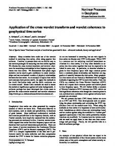
Again, assuming the models are correct, this subtraction restores asymptotic unbiasedness. The corresponding confidence regions (this is 2-D now) are depicted on Figure 8. How to choose the scale of the wavelet for best performance? Since the physical source is point-like, recorded sources look like the impulse response of the detector, i.e., the PSF. Hence the best choice for the scale parameter 17
Declination
200 30
180 25 160
140 20 120 15
100 10
80 5 60
40 0 20 -5
0 0
70
50
60
100
50
150
40
200
30
250
20 300 10 350 Right Ascension
Figure 8: Detected sources using the wavelet analysis of the EGRET viewing period 21.0 for E>100 MeV, the contours give the significance level from 4 to 16 σ. Superimposed stars give the positions of the third EGRET catalog sources detected over 4 σ [21]. is that leading to a wavelet with width comparable to the one of the PSF. This width does not vary much from source to source, it only depends on the energy of the incoming photons. A source emitting proportionally more at high energies than low energies is said to be ‘hard’, or to have a low spectral index and has a rather peaked PSF: It is best detected at small scale. On the contrary, a ‘soft’ source has a rather flat PSF and is best detected at a larger scale. This dependence of the optimal scale parameter on the spectral index is illustrated on Figure 9. Most of the 270 EGRET sources are not identified. The intrinsic resolution of high energy gamma-ray detectors is not good enough to provide strong constraints on the source position; it is therefore difficult to find counterparts at other wavelengths. Their nature is still a mystery that the next generation telescope GLAST will help to solve. A large fraction of identified sources consists in active galaxies whose nucleus is a massive black hole (up to 109 MSun ) surrounded by an accretion disk of matter falling in the gravitational well. Besides, strong jets of ultra-relativistic matter and radiation are emitted perpendicularly to the disk. Active galactic nuclei (AGN) detected in gamma-rays above 100 MeV have a jet pointed towards the Earth. Their emission is very variable, so that they are often undetected when they are in a quiescent state and then, in a short time, they become very bright. Viewing period 21.0 is a high latitude observation in which an AGN is in flaring state; 3EG J0237+1635 was detected at 10 σ in [21] and is 16σ here. Several other sources are also present above 4 σ. The procedure described above has been applied and results are shown in Figure 8. One can see that all but one sources are seen. One should also note that the bright AGN position is slightly wrong, because of the presence of a faint source in the vicinity that is not detected. To detect this kind of source, the algorithm must be applied a second time after the addition of the significant sources to the background. 18
Number of σ
7
6
5
4
3
2 0
2
4
6
8 10 Scale parameter a
Figure 9: Significance for the detection of a source, expressed in number of sigmas, as a function of the scale parameter of the wavelet. The wavelet is centered at the position of the source. Each curve refers to a different spectral index, from lower (peaked curve) to higher (flat curve). The position of the maxima of these curves changes as the spectral index changes. 4.3
Conclusion
Our attempt at developing an alternative method to the usual maximum likelihood estimation will probably prove to be relevant in the years to come. Indeed, the next generation gamma-ray telescope, GLAST, is to be launched in March 2006 and its complexity (parameters to take into account, volume of the data stream) will make it impossible to build a source catalog following EGRET’s old-school procedure. The algorithms must be made more efficient in some way. Wavelets will not be the key to the whole problem, of course, but will hopefully help develop alternative viewpoints.
Appendix: The 2-D continuous wavelet transform Given an image I, that is, a finite energy signal I ∈ L2 (R2 , d2�x ), its two-dimensional continuous wavelet transform, with respect to the wavelet ψ, is defined as the scalar product, in the sense of L2 (R2 , d2�x ), of I with ψ: � d2�x ψ�b a θ (�x) I(�x) , (A.1) WI (�b, a, θ) = R2
where the overbar denotes the complex conjugation, ψ�b a θ is a copy of ψ translated by �b ∈ R2 , dilated by a factor a > 0, and rotated by an angle θ ∈ [0, 2π], that is,
� 1 1 −1 � (A.2) r (�x − b) , ψ�b a θ (�x) = 2 ψ a a θ with rθ the rotation matrix of angle θ. Notice that ψ�b a θ is L1 (R2 , d2�x ) normalized, i.e. �ψ�b a θ �1 = �ψ�1 . 19
The wavelet function ψ must be well localized both in position �x and in spatial frequency �k, which means that it is (numerically) negligible outside of bounded subsets of R2 in each variable. In addition, to guarantee that no information is lost in the coefficients WI , that is, to be able to reconstruct I from these elements, we must impose an admissibility requirement on ψ, namely � ˆ �k)|2 |ψ( 2 d2�k < ∞. (A.3) cψ ≡ (2π) �k�2 R2 Under mild regularity assumptions, the admissibility condition (A.3) implies the following easier one, which simply means that the function ψ has zero mean: � � �0) = 0 ⇐⇒ ψ( d2�x ψ(�x) = 0. (A.4) R2
Strictly speaking, the condition (A.4) is only necessary, but in fact it is almost sufficient (see [14] for a precise mathematical statement), and for all practical purposes (A.4) may be taken as admissibility condition. In this case, the function ψ is called a wavelet. Combining the admissibility condition with the support properties of ψ, one naturally interprets the CWT as a local (bandpass) filter in all four variables (�b, a, θ), in other words, the CWT sees the content of I, if any, at the location �b, at the scale a and in the direction θ. Equivalently, the wavelet coefficient WI is strong where the image I resembles locally ψ�b a θ . Starting from the definition, a straightforward calculation yields a Plancherel relation for the CWT, which manifests the fact that no energy is lost in the CWT parameter space: � � � � 2π da 1 2 2 2 �I� = d �x |I(�x)| = d2�b (A.5) dθ |WI (�b, a, θ)|2 . cψ R 2 R + 0 a R2 From this relation, which justifies the admissibility condition cψ < ∞, |WI |2 can be interpreted as an energy density in the CWT space (and thus the support property of the wavelet means that most of the energy of ψ and ψ� lives in the support of these functions). We will denote this energy density as EI (�b, a, θ) = |WI (�b, a, θ)|2 .
(A.6)
As a consequence of the Plancherel relation (A.5), one obtains an exact reconstruction formula of the image from its wavelet transform: ��� da −1 I(�x) = cψ (A.7) dθ ψ�b,a,θ (�x) WI (�b, a, θ). d2�b a Now, if the wavelet ψ is rotation invariant, as will be the case in most applications discussed below, the rotation matrix rθ has no effect and we get ψ�b a θ (�x) ≡ ψ�b a (�x) = a−2 ψ(a−1 (�x − �b)). Thus the formulas simplify to � � d2�x ψ�b a (�x) I(�x) , (A.8) WI (b, a) = R2
I(�x) = 2π
c−1 ψ
�� d2�b 20
da ψ� (�x) WI (�b, a). a b,a
(A.9)
We emphasize that the CWT transforms a two-dimensional image into a function depending on four variables (two dimensions for �b, one for a and θ), and it is therefore highly redundant. This property is actually very useful, since it enables the CWT to discriminate between an object living at a given scale and a larger event at the same location. We will exploit this in the analysis of EIT images, in Section 3. Among the isotropic or rotation invariant wavelets, the simplest one is the so-called Mexican hat, namely the Laplacian of a Gaussian (thus also called LOG wavelet): ψH (�x) = −∆ exp(− 12 |�x|2 ) = (2 − |�x|2 ) exp(− 12 |�x|2 ).
(A.10)
In Fourier space, this gives ψ�H (�k) = |�k|2 exp(− 12 |�k|2 ) .
(A.11)
Thus, the Mexican hat is a real, isotropic, wavelet, well localized both in space (the essential support of ψH is a disc with radius proportional to the scale) and in the spatial frequency plane (the essential support of ψ�H is an annulus with inner and outer radii proportional to the inverse of the scale). As a consequence, the CWT of an image I with respect to ψH is simply the Laplacian of a smoothed version of the original image I by a Gaussian of size a. Thus the maxima of EI detect the maxima of the curvature of I at a given scale, that is, mainly its peaks. In addition, this wavelet has two vanishing moments: � � 2 d �x ψH (�x) = d2�x xk ψH (�x) = 0, k = 1, 2. (A.12) R2
R2
It is therefore insensitive to constant and linear components in the background (for instance, a smooth gradient in the intensity of the image). Another isotropic wavelet, introduced in [18] under the rather funny name of Pet hat, is defined in Fourier space as � |�k| 2 π � � �k) = cos ( 2 log2 2π ) : π < |k| < 4π ψ( (A.13) 0 : |�k| < π, |�k| > 4π. This wavelet has a better resolving power in scale than the Mexican hat. For some applications described in the text, one has to consider the Universe globally, taking into account its spherical shape. This means that one should then use a spherical wavelet transform. While a discrete approach to the latter (spherical Haar wavelets) was designed by Sweldens [35], a full continuous CWT on the 2-sphere S 2 was constructed in [5]. The idea is simply to take the plane R2 as the tangent plane at the North Pole of S 2 and lift functions on R2 to functions on S 2 by inverse stereographic projection. Introducing polar coordinates both on the plane and on the sphere, the correspondence reads: θ S 2 � (θ, ϕ) ⇐⇒ (r, ϕ) ≡ (2 tan , ϕ). 2 For square integrable functions, this leads to a unitary map between the respective Hilbert spaces, I −1 : L2 (R2 , d2�x ) → L2 (S 2 , sin θ dθ dϕ), namely, (I −1 f )(θ, ϕ) =
θ 2 f (2 tan , ϕ). 1 + cos θ 2 21
(A.14)
In the case of an isotropic wavelet ψ(r), with r = |�x|, the correspondence is simply (I −1 ψ)(θ) =
θ 2 ψ(2 tan ). 1 + cos θ 2
(A.15)
Then, choosing for ψ the Mexican hat wavelet ψH , one gets the spherical Mexican hat wavelet.
References [1] J-P. Antoine, P. Carrette, R. Murenzi, and B. Piette, Image analysis with twodimensional continuous wavelet transform, Signal Proc., 31 (1993) 241–272 [2] J-P. Antoine and R. Murenzi, Two-dimensional wavelet analysis in image processing, Physicalia Mag., 16 (1994) 105–134 [3] J-P. Antoine, R. Murenzi, and P. Vandergheynst, Directional wavelets revisited: Cauchy wavelets and symmetry detection in patterns, Appl. Comput. Harmon. Anal., 6 (1999) 314–345 [4] J-P. Antoine, The 2-D wavelet transform, physical applications and generalizations, in Wavelets in Physics, pp. 23–75; J. C. van den Berg (ed.), Cambridge Univ. Press, Cambridge, 1999 [5] J-P. Antoine and P. Vandergheynst, Wavelets on the 2-sphere: A group-theoretical approach, Appl. Comput. Harmon. Anal., 7 (1999) 262–291 [6] R.B. Barreiro, M.P. Hobson, A.N. Lasenby, A.J. Banday, K.M. Gorski, and G. Hinshaw, Testing the Gaussianity of the COBE DMR data with spherical wavelets, Mon. Not. R. Astron. Soc., 318 (2000) 475–481 [7] A. Bijaoui and F. Ru´e, A multiscale vision model adapted to the astronomical images, Signal Proc., 46 (1995) 345–362 [8] A. Bijaoui, E. Slezak, F. Ru´e, and E. Lega, Wavelets and the study of the distant Universe, Proc. IEEE, 84 (1996) 670–679 [9] A. Bijaoui, Wavelets and astrophysical applications, in Wavelets in Physics, pp. 77– 115; J. C. van den Berg (ed.), Cambridge Univ. Press, Cambridge, 1999 [10] A. Bijaoui and G. Jammal, On the distribution of the wavelet coefficient for a Poisson noise, Signal Proc., 81 (2001) 1789–1800 [11] L. Cay`on, J.L. Sanz, R.B. Barreiro, E. Martinez-Gonzalez, P. Vielva, L. Toffolati, J. Silk, J.M. Diego, and F. Arg¨ ueso, Isotropic wavelets: A powerful tool to extract point sources from cosmic microwave background maps, Mon. Not. R. Astron. Soc., 315 (2000) 757–761
22
[12] L. Cay`on, J.L. Sanz, E. Martinez-Gonzalez, A.J. Banday, F. Arg¨ ueso, J.E. Gallegos, K.M. Gorski, and G. Hinshaw, Spherical Mexican Hat wavelet: An application to detect non-Gaussianity in the COBE-DMR maps, Mon. Not. R. Astron. Soc., 326 (2001) 1243–1249 [13] F. Damiani, A. Maggio, G. Micela, and S. Sciortino, A method based on wavelet transforms for source detection in photon-counting detector images. I. Theory and general properties, Astroph. J., 483 (1997) 350–369; II. Application to ROSAT PSPC images, ibid, 483 (1997) 370–389 [14] I. Daubechies, Ten Lectures on Wavelets, SIAM, Philadelphia, PA, 1992 [15] J-P. Delaboudini`ere et al., EIT: Extreme-ultraviolet imaging telescope for the SoHO mission, Solar Physics, 175 (1995) 291–312 [16] W.T. Eadie, D. Drijard, F.E. James, M. Ross, and B. Sadoulet, Statistical Methods in Experimental Physics, North Holland, Amsterdam, London, 1971 [17] P. Frick, R. Beck, A. Shukurov, D. Sokoloff, M. Ehle, and J. Kamphuis, Magnetic and optical spiral arms in the galaxy NGC 6946, Mon. Not. R. Astron. Soc., 318 (2000) 925–937 [18] P. Frick, R. Beck, E.M. Berkhuijsen, and I. Patrickeyev, Scaling and correlation analysis of galactic images, Mon. Not. R. Astron. Soc., 327 (2001) 1145–1157 [19] C. Gonnet and B. Torr´esani, Local frequency analysis with two-dimensional wavelet transform, Signal Proc., 37 (1994) 389–404 [20] S.A. Grebenev, W. Forman, C. Jones, and S. Murray, Wavelet transform analysis of the small-scale X-ray structure of the cluster Abell 1367, Astroph. J., 445 (1995) 607–623 [21] R.C. Hartman et al., The third EGRET catalog of high-energy gamma-ray sources, Astroph. J. Suppl., 123 (1999) 79–202 [22] J-F. Hochedez, F. Clette, E. Verwichte, D. Berghmans, and P. Cugnon. Mid-term variations in the extreme UV corona: The EIT/SoHO perspective. In Proc. 1st Solar & Space Weather Euroconference, “The Solar Cycle and Terrestrial Climate”, Santa Cruz de Tenerife, Spain, 25-29 September 2000 (ESA SP 463, December 2000) [23] S.D. Hunter et al., EGRET observation of the diffuse gamma-ray emission from the galactic plane, Astroph. J., 481 (1997) 205–240 [24] S.G. Mallat and S. Zhong, Characterization of signals from multiscale edges, IEEE Trans. Pattern Anal. Machine Intell., 14 (1926) 710–732 [25] E. Lega, A. Bijaoui, J.M. Alimi, and H. Scholl, A morphological indicator for comparing simulated cosmological scenarios with observations, Astron. Astroph., 309 (1996) 23–29 23
[26] E. Martinez-Gonzalez, J.E. Gallegos, F. Arg¨ ueso, L. Cay`on, and J.L. Sanz, The performance of spherical wavelets to detect non-Gaussianity in the CMB sky , Mon. Not. R. Astron. Soc., (to appear); preprint arXiv:astro:ph/0111284 (Nov. 2001) [27] J.R. Mattox et al., The likelihood analysis of EGRET data, Astroph. J., 461 (1996) 396–407 [28] D. Moses and al. EIT observations of the Extreme Ultraviolet Sun, Solar Physics, 175 (1997) 571–599 [29] F. Portier-Fozzani, B. Vandame, A. Bijaoui, and A.J. Maucherat, A Multiscale Vision Model applied to analyze EIT images of the solar corona, Solar Physics, 201 (2001) 271–288 [30] J.L. Sanz, R.B. Barreiro, L. Cay`on, E. Martinez-Gonzalez, G.A. Ruiz, F.J. Diaz, F. Arg¨ ueso, J. Silk, and L. Toffolati, Analysis of CMB maps with 2D wavelets, Astron. Astroph., Suppl. Series 140 (1999) 99–105 [31] J.L. Sanz, F. Arg¨ ueso, L. Cay`on, E. Martinez-Gonzalez, R.B. Barreiro, and L. Toffolati, Wavelets applied to cosmic microwave background maps: A multiresolution analysis for denoising, Mon. Not. R. Astron. Soc. 309 (1999) 672–680 [32] E. Slezak, A. Bijaoui, and G. Mars, Identification of structures from galaxy counts. Use of the wavelet transform, Astron. Astroph. 227 (1990) 301–316 [33] E. Slezak, V. de Lapparent, and A. Bijaoui, Objective detection of voids and highdensity structures in the 1st CfA redshift survey slice, Astroph. J., 409 (1993) 517– 529 [34] J.L. Starck and M. Pierre, Structure detection in low-intensity X-ray images, Astron. Astroph. Suppl. Ser. 128 (1998) 397-407 [35] P. Schr¨oder and W. Sweldens, Spherical wavelets: Efficiently representing functions on the sphere, Computer Graphics Proc. (SIGGRAPH95), ACM Siggraph 1995, pp. 161–175 [36] R. Terrier, L. Demanet, I. Grenier, and J-P. Antoine, Wavelet analysis of EGRET data, in Proc. 27th International Cosmic Ray Conference, Hamburg, Germany, August 2001 [37] P. Vielva, R.B. Barreiro, M.P. Hobson, E. Martinez-Gonzalez, A.N. Lasenby, J.L. Sanz, and L. Toffolati, Combining maximum-entropy and the Mexican hat wavelet to reconstruct the microwave sky, Mon. Not. R. Astron. Soc. 328 (2001) 1–16.
24