1 Science Park Road, #01-01 The Capricorn. Singapore ... Application of the improved finite element-fast multipole method. 51. V n r r. E inc. H inc. Js. Ms. PEC.
Progress In Electromagnetics Research, PIER 47, 49–60, 2004
APPLICATION OF THE IMPROVED FINITE ELEMENT-FAST MULTIPOLE METHOD TO LARGE SCATTERING PROBLEMS X. C. Wei, E. P. Li, and Y. J. Zhang Computational Electromagnetics and Electronics Division Institute of High Performance Computing National University of Singapore 1 Science Park Road, #01-01 The Capricorn Singapore Science Park II, Singapore 117528 Abstract—The finite element hybridized with the boundary integral method is a powerful technique to solve the scattering problem, especially when the fast multipole method is employed to accelerate the matrix-vector multiplication in the boundary integral method. In this paper, the multifrontal method is used to calculate the triangular factorization of the ill conditioned finite element matrix in this hybrid method. This improves the spectral property of the whole matrix and makes the hybrid method converge very fast. Through some numerical examples including the scattering from a real-life aircraft with an engine, the accuracy and efficiency of this improved hybrid method are demonstrated.
1 Introduction 2 Formula of the Improved Hybrid Method 3 Numerical Examples 4 Conclusions References 1. INTRODUCTION The accurate and efficient evaluation of the scattering from a large and complex object, such as an aircraft with the engine and coating, is of great interest in engineering. The finite element hybridized
50
Wei, Li, and Zhang
with the boundary integral equation method is approved to be a powerful numerical method for such complex problem simulation [1]. Meanwhile, the finite element method is very suitable to deal with the complex inhomogeneous materials, and the boundary integral equation is employed to truncate the computational region of the finite element method for the open region problem such as the scattering. Then, the matrices generated from the finite element method and the boundary integral equation are combined together and solved using an iterative solver such as the biconjugate gradient method (BiCG). This hybrid method is more accurate than the finite element method using the absorbing boundary condition (ABC), because the boundary integral equation is exact, and the truncation surface can be placed on the surface of the scatterer to reduce the whole computational domain. The boundary integral equation is discretized using the moment methods, which leads to a dense and large coefficient matrix. Some approaches had been employed to solve this matrix efficiently, such as the wavelet transform [2, 3] and the impedance matrix localization method (IML) [4, 5]. Recently, the fast multipole method (FMM) [6] (or its multilevel version MLFMA [7]) is applied to accelerate the computation of the boundary integral equation. The computational complexity of the matrix-vector multiplication and the memory requirement of the boundary integral equation are reduced from the original o(N 2 ) to o(N 1.5 ) using the fast multipole method (or o(N log N ) using its multilevel version), where N denotes the number of unknowns in the boundary integral equation. So the performance of the hybrid method is greatly improved in solving the large scattering problems. Unfortunately, this FEM-FMM hybrid method still suffers from a very slow convergence rate, especially for the complex media. This is due to the badly conditioned matrix arising from the finite element method, which pollutes the spectral property of the whole FEM-FMM matrix equation. So far, several methods are proposed to improve the convergence behavior of this FEM-FMM method. In [8], the variant of the conventional biconjugate gradient method, named BICGSTAB (l), combined with the preconditioner are employed to solve the whole equations quickly. And in [9], the finite element matrix is solved directly using a package named SuperLU, after that, it is implemented into the FEM-FMM method in order to make the whole matrix equation better conditioned. In [10], a ABC-based preconditioner is proposed, where, the preconditioner is constructed using the absorbing boundary condition placed on the truncation surface. In this paper, the multifrontal method [11] is applied to perform the triangular (LU) factorization of the finite element matrix. Here, the efficient
Application of the improved finite element-fast multipole method
51
E inc H inc Ms
Js
n
s2 PEC
εr
V
µr S1
Figure 1. The scatterer. package from the Harwell Subroutine Library (HSL) is implemented into the conventional FEM-FMM method. This package makes a full use of the sparsity and symmetry pattern of the finite element matrix, and the factorization is performed by calls to the Basic Linear Algebra Subprograms (BLAS). So the iteration number and computing time of this improved FEM-FMM method are greatly reduced, while the additional computing time and store requirement due to the LU factorization are kept small. The accuracy and efficiency of this improved FEM-FMM method are verified using some numerical examples. Through the evaluation of a real-life aircraft with the engine, this enhanced FEM-FMM method is proved to be efficient for the practical engineering application. In the following, Section 2 discusses the formulation of the improved FEM-FMM method and the implementation of the LU factorization. Section 3 illustrates some numerical examples and Section 4 is the conclusions. 2. FORMULA OF THE IMPROVED HYBRID METHOD As shown in Fig. 1, let us consider the problem of the electromagnetic scattering by an arbitrarily shaped scatterer characterized by the relative permittivity and permeability (εr , µr ). In this paper, without loss of the general sense, this scatterer can be partially covered by the perfect electric conducting (PEC) sheets, so the whole surface S of the scatterer is divided into the non-PEC surface S1 and the PEC surface S2 . The electric fields satisfy the variational equation with the
52
Wei, Li, and Zhang
function given by [1] F (E) =
1 2
��� � V
�
1 (∇ × E V ) · (∇ × E V ) − k02 εr E V · E V dV µr
��
ˆ (E S × H S ) · ndS
+jk0 η0
(1)
S
Where, the total unknown electric field E is divided into E S and E V , which denote the electric field on the surface S and inside the volume V respectively. H S represents the magnetic field on S. k0 is the free space wave number, η0 = 120π is the free space intrinsic impedance, ˆ denotes the outside unit vector normal to S. It should be noted and n that the surface integral in Equation (1) is zero on the PEC surface S2 . Equation (1) is discretized into the linear equations using the finite element method. Where, E S and E V are expanded using the edgebased functions defined on the tetrahedron. These linear equations cannot be solved, since H S in Equation (1) is still unknown. So a boundary condition (Here it is the H S ) should be placed on S to solve these finite element linear equations. The following boundary integral equations are employed as the required boundary condition ��
1 ˆ × M S (r) + E inc n t (r) = 2
∇G × M S (r � )dS �
S
��
+jη0 k0
S
��
1 J S (r � )GdS � + ∇ k0
t
∇�· J S (r � )GdS �
S
�� 1 inc � � ˆ × J S (r) − H t (r) = − n ∇G × J S (r )dS
(2a)
t
2
S
��
1 +j k0 η0
S
��
t
1 M S (r � )GdS � + ∇ ∇�· M S (r � )GdS � (2b) k0 S
inc
inc
t
Where, as shown in Fig. 1, E and H denote the incident electric and magnetic fields on S respectively. J S and M S denote the unknown equivalent electric and magnetic currents on S respectively. −jk0 |r−r� | is the free space Green’s function. t denotes the G = e 4π|r−r �| compoment tangential to S. Equation (2a) is the electric field integral equation and Equation (2b) is the magnetic field integral equation. In order to
Application of the improved finite element-fast multipole method
53
avoid the interior resonance for a closed scatterer, they are combined to form the combined field integral equation. Here, the triangular basis function f i is used to expand J S and M S . Equation (2a) is tested ˆ × f i . Meanwhile, the using f i and Equation (2b) is tested using n self-singularity and near-singularity in these integrals are calculated analytically [12] to insure the accuracy of these integrals. Equations (1), (2a) and (2b) can be combined together using the following relations ˆ × H S (r), J S (r) = n
ˆ M S (r) = E S (r) × n
r∈S
(3)
So, the final matrices equation can be obtained as
�
[A] [Y 0]
� � � ES � 0 EV [0] 0 � � = J S1 [e]
C 0 [Z]
(4)
J S2
Where, matrices A and C are finite element matrices generated from Equation (1), and matrices Y and Z are boundary integral matrices generated from the combination of Equations (2a) and (2b). J S is divided into J S1 and J S2 , which denote the equivalent electric currents on S1 and S2 respectively. e denotes the excitation vector due to E inc and H inc . It should be noted that using the relations in Equation (3), M S and H S are represented by E S and J S1 in Equation (4) respectively. For a large scattering problem, Equaiton (4) is usaully solved using an iterative solver. Matrices A and C are sparse, and A is symmetric. Matrices Y and Z are full. The matrixvector multiplication and store requirement of matrices Y and Z are expensive, which can be reduced using the fast multipole method [6, 7]. Equation (4) still has a bottleneck, which is the low convergence rate. This is because that the matrix A is ill conditioned, which pollutes the spectral property of the whole coefficient matrix in Equation (4). To eliminate this difficult, in this paper, the multifrontal method [7] is employed to do the LU factorization of A as following [A] = [L][D][L]T
(5)
Where, [L] is the unit lower triangular matrix and [D] is the diagonal matrix. T in Equation (5) denotes the transpose. Substituting Equation (5) into Equation (4), the improved matrices equation can be obtained as
−T
[Z] − [Y 0] · [L]
−1
· [D]
−1
· [L]
�
·
C 0 0 0
�� �
J S1 J S2
�
= [e]
(6)
54
Wei, Li, and Zhang
This matrix equation is better conditioned than the original FEMFMM Equation (4), so it can be quickly solved using the biconjugate gradient method. Two additional costs should be considered for this improved FEMFMM method, which are the computing time and store requirement for the LU factorization. In this paper, the efficient package from the Harwell Subroutine Library is employed to perform the LU factorization. This package makes a full use of the sparsity and symmetry pattern of the matrix A. Where, only half of the elements in the matrix A are required to be stored. And, before performing the numerical factorization, it performs the symbolic factorization to minimize the amount of “fill-in” in the factor matrix L. This reduces the additional memory requirement. On the other hand, this LU package uses the Basic Linear Algebra Subprograms to do the factorization. Basic Linear Algebra Subprograms provide the vector/matrix operations that can be optimized for different computer architectures to achieve high efficiency. So the calculation of the LU factorization is very fast. In the following examples, this additional computing time even can be ignored compared with the total computing time. 3. NUMERICAL EXAMPLES In this section, the performance of the improved FEM-FMM method is verified using some numerical examples. The first scatterer is a two-layer coated sphere [13], which is used here to verify our code. Where, the conducting sphere has a radius of 0.75λ, and λ denotes the wavelength. The thickness of each layer is 0.05λ. The outer layer has a relative permittivity εr1 = 2 − j1 and a relative permeability µr1 = 3 − j2. The inner layer has a relative permittivity εr2 = 3 − j2 and a relative permeability µr2 = 2 − j1. Fig. 2 shows the bistatic radar cross section (RCS) obtained using the improved FEM-FMM method (denote by FEMFMM-LU), the conventional FEM-FMM method (denoted by FEMFMM), and the Mie series. The iteration numbers of these methods are listed in Table 1. From Fig. 2 we can see that there is a good agreement between the improved FEM-FMM method and the Mie series. While the result of the conventional FEM-FMM method is not accurate for 0◦ ≤ θ ≤ 90◦ . The reason is that the media of these two layers are high contrast, which leads to a very ill conditioned finite element matrix. This matrix not only greatly pulls down the convergence of the conventional FEM-FMM method, but also results in an inaccurate solution. While, with the help of the multifrontal
Application of the improved finite element-fast multipole method
55
Table 1. Unknowns number, memory requirement, iteration number and computing time for three scatterers. Scatters
Unknowns Number
Memory (GB)
Iteration Number Total Computing LU Time (Min.) Factorization FEM-FMM- FEMFEMFEMFEMFEMTime (Min.)
Coated Sphere Microstrip Array Aircraft with the Engine
34 482(FEM) 15 876(FMM) 48 346(FEM) 24 722(FMM) 28 663(FEM) 25 320(FMM)
FMM
FMM-LU
FMM
0.85
LU
FMM FMM-LU
0.7
76
10 166
20
925
0.27
1.31
1.22
551
2 268
86
321
0.23
1.91
1186
935
0.21
Bistatic RCS dB
30
FEM-FMM-LU FEM-FMM Mie
15
0
-15 0
45
90
135
180
θ Degree Figure 2. The bistatic RCS of the two-layer coated sphere using the improved FEM-FMM method, the conventional FEM-FMM method, and the Mie series. method, the improved FEM-FMM method can provide an accurate result, and with the same error tolerance its iteration is only about 1% of that of the conventional FEM-FMM method. The second scatterer is a finite three by three microstrip array mounted on a two-layer substitute as shown in Fig. 3. The upper layer in which the patches are embedded has the thickness of 0.03048λ, and is filled using G10 with εr1 = 3.8 − j0.01482 and µr1 = 1. The lower layer on the top of the finite ground plane has the thickness of 0.015748λ, and is filled using Duroid 5880 with εr2 = 2.22 − j0.001998 and µr2 = 1. The size of each patch is 0.732λ × 0.52λ. The size of the finite ground plane is 3.396λ × 2.76λ. The distance between each patch
56
Wei, Li, and Zhang
y
0
x
Figure 3. The three by three microstrip array. FEM-FMM-LU FEM-FMM HFSS
Bistatic RCS dB
40
20
0
-20 -90
-45
θ
0
45
90
Degree
Figure 4. The bistatic RCS of the three by three microstrip array in y-z plane using the improved FEM-FMM method, the conventional FEM-FMM method, and Ansoft HFSS software. is 0.3λ. Fig. 4 shows the bistatic RCS of this array in the y-z plane for a plane wave incident along −z-axis with the y-polarized electric field. The result using the Ansoft HFSS software is also shown in Fig. 4 for the verification. The agreement between these three results is good. The last scatterer is an aircraft with an engine as shown in Fig. 5. Where, the engine is modeled as an open and deep cavity. This aircraft has a length of 10.9λ and a wingspan of 6.9λ. The length of the engine
Application of the improved finite element-fast multipole method
57
Figure 5. The aircraft with an engine. (a) y-z plane. (b) x-z plane. With the engine Without the engine
Bistatic RCS dB
40
Nose
Tail 20
0
-20 0
90
θ
180
270
360
Degree
Figure 6. The bistatic RCS of the aircraft with the engine and without the engine in x-z plane. is 7.3λ. Fig. 6 shows the bistatic RCS of this aircraft in x-z plane using the improved FEM-FMM method. Where, the incident wave is along −x-axis with the z-polarized electric field as shown in Fig. 5(b). In Fig. 6, the bistatic RCS of the aircraft without the engine using only the fast multipole method is also shown for the comparison, where, the ports of the engine are closed and the whole aircraft is treated as a closed PEC scatterer. The maximum RCS difference between these
58
Wei, Li, and Zhang
two models occurs at the tail, where θ = 90◦ . While for other angles far away from 90◦ , these two models present the similar scattering pattern. This reveals that the engine plays an important role on the scattering, when the incident wave is toward the import/export of the engine. For such incident directions, the engine should be considered together with the aircraft to give an accurate result. For this aircraft with the engine, there are totally 54 K unknowns. With the help of the fast multipole method, this large problem can be solved on a single computer with a 1.3 GHz CPU and 2 GB memory. Table 1 lists the number of unknowns, the memory requirement, the iteration number and computing time for above three scatterers. From this table we can see that with the help of the LU factorization, the iteration numbers and the total computing time of the improved FEM-FMM method are dramatically reduced compared with those of the conventional FEM-FMM method. The additional store requirement due to the LU factorization is less than 3% of that of the conventional FEM-FMM method, although the unknowns of the finite element method are more than those of the boundary integral. This is because that the finite element matrix is symmetric and sparse, and usually the boundary integral equation occupies the largest memory in the FEM-FMM method. At the same time, the additional computing time due to the LU factorization only takes less than 1% of the total computing time of the improved FEM-FMM method, so that this additional cost can be ignored. From the iteration numbers in Table 1 we can see that the more complicated the scatterer, the more the iteration. According to our experiences, for the complex real-life scatterer such as the aircraft, not only the finite element matrix but also the boundary integral matrix is very badly conditioned, because there are many reflections and diffractions between different structures of the scatterer. In such cases, the conventional FEM-FMM method will take too long to converge, so it is not employed for the aircraft in Table 1. 4. CONCLUSIONS The finite element hybridized with the fast multipole method is employed to solve the scattering problems. Where, the multifrontal method is used to calculate the LU factorization of the finite element matrix. The computing time of this improved hybrid method is greatly reduce compared with that of the conventional hybrid method. Some numerical examples are presented to show the accuracy and efficiency of this improved hybrid method.
Application of the improved finite element-fast multipole method
59
REFERENCES 1. Jin, J. M., The Finite Element Method in Electromagnetics, Second edition, Wiley, New York, 2002. 2. Xiang, X. and Y. Lu, “A hybrid FEM/BEM/WTM approach for fast solution of scattering from cylindrical scatters with arbitrary cross sections,” J. Electromag. Wave Applicat., Vol. 13, No. 6, 811–812, 1999. 3. Wei, X. C., E. P. Li, and C. H. Liang, “Fast solution for large scale electromagnetic scattering problems using wavelet transform and its precondition,” J. Electromag. Wave Applicat., Vol. 17, No. 4, 611–613, 2003. 4. Canning, F. X., “The impedance matrix localization method (IML) for MM calculation,” IEEE Trans. Antennas Propagat. Mag., Vol. 32, No. 5, l8–30, Oct. 1990. 5. Canning, F. X., “Transformations that produce a sparse moment method matrix,” J. Electromag. Wave Applicat., Vol. 4, No. 9, 893–913, 1990. 6. Rokhlin, V., “Rapid solution of integral equations of scattering theory in two dimensions,” J. Comput. Phys., Vol. 86, 414–439, Feb. 1990. 7. Song, J. M. and W. C. Chew, “Multilevel fast-multipole algorithm for solving combined field integral equations of electromagnetic scattering,” Micro. and Opt. Tech. Lett., Vol. 10, No. 1, 14–19, Sept. 1995. 8. Topsakal, E., R. Kindt, K. Sertel, and J. Volakis, “Evaluation of the BICGSTAB(l) algorithm for the finite-element/boundaryintegral method,” IEEE Trans. Antennas Propagat. Mag., Vol. 43, No. 6, 124–131, Dec. 2001. 9. Sheng, X. Q. and E. K. N. Yung, “Implementation and experiments of a hybrid algorithm of the MLFMA-enhanced FE-BI method for open-region inhomogeneous electromagnetic problems,” IEEE Trans. Antennas Propagat., Vol. 50, No. 2, 163– 167, Feb. 2002. 10. Jian, L. and J. M. Jin, “A highly effective preconditioner for solving the finite element-boundary integral matrix equation of 3-D scattering,” IEEE Trans. Antennas Propagat., Vol. 50, No. 9, 1212–1221, Sept. 2002. 11. Liu, J. W. H., “The multifrontal method for sparse matrix solution: theory and practice,” SIAM Review, Vol. 34, No. 1, 82– 109, Mar. 1992. 12. Graglia, R. D., “On the numerical integration of the linear shape
60
Wei, Li, and Zhang
functions times the 3-D Green’s function or its gradient on a plane triangle,” IEEE Trans. Antennas Propagat., Vol. 41, No. 10, 1448– 1455, Oct. 1993. 13. Sheng, X. Q., J. M. Jin, J. M. Song, C. C. Lu, and W. C. Chew, “On the formulation of hybrid finite-element and boundaryintegral methods for 3-D scattering,” IEEE Trans. Antennas Propagat., Vol. 46, No. 3, 303–311, Mar. 1998.
X. C. Wei received the Ph.D. degree in electromagnetic field and microwave technology from Xidian University, Xi’an, China, in 2001. Now, he has been with the Institute of High Performance Computing, National University of Singapore, as a post-doctoral research fellow. His main research interest is in the analysis of electromagnetic compatibility, electromagnetic wave propagation and scattering, and the development of new numerical techniques for electromagnetic computation. E. P. Li received his Ph.D. from Sheffield Hallam University in electrical engineering in 1992. He has been a senior research fellow and project manager/director in Singapore Research Institute and private company from 1993 to 1999. Dr. Li is an elected Deputy Chairman for IEEE EMC Chapter in Singapore. He has published over 30 papers in international journals and conferences. His research interests include EMC/EMI, computational electromagnetic, high speed electronic modeling and Microwave engineering. Y. J. Zhang received the Ph.D. from Beijing University in physical electronics. From 1999 to 2001, he worked as a research fellow in Tsinghua University, China. Currently, he is a senior research fellow in the Institute of High Performance Computing, National University of Singapore. His research interests include fast algorithms in electromagnetics and its applications in radar cross section prediction, microwave devices simulation and antennas modeling.