1018
JOURNAL OF ATMOSPHERIC AND OCEANIC TECHNOLOGY
VOLUME 25
Application of the Sequential Three-Dimensional Variational Method to Assimilating SST in a Global Ocean Model ZHONGJIE HE College of Physical and Environmental Oceanography, Ocean University of China, Qingdao, and National Marine Data and Information Service, State Oceanic Administration, Tianjin, China
YUANFU XIE NOAA/Earth System Research Laboratory, Boulder, Colorado
WEI LI College of Physical and Environmental Oceanography, Ocean University of China, Qingdao, and National Marine Data and Information Service, State Oceanic Administration, Tianjin, China
DONG LI, GUIJUN HAN, KEXIU LIU,
AND
JIRUI MA
National Marine Data and Information Service, State Oceanic Administration, Tianjin, China (Manuscript received 7 November 2006, in final form 15 June 2007) ABSTRACT A recursive filter or parameterized curve fitting technique is usually used in a three-dimensional variational data assimilation (3DVAR) scheme to approximate the background error covariance, which can only represent the errors of an ocean field over a predetermined scale. Without an accurate flow-dependent error covariance that is also local and time dependent, a 3DVAR system may not provide good analyses because it is optimal only under the assumption of an accurate covariance. In this study, a sequential 3DVAR (S3DVAR) is formulated in model grid space to examine if there is useful information that can be extracted from the observation. This formulation is composed of a series of 3DVARs, each of which uses recursive filters with different length scales. It can provide an inhomogeneous and anisotropic analysis for the wavelengths that can be resolved by the observation network, just as with the conventional Barnes analysis or successive corrections. Being a variational formulation, S3DVAR can deal with data globally with an explicit specification of the observation errors; explicit physical balances or constraints; and advanced datasets, such as satellite and radar. Even though the S3DVAR analysis can be viewed as a set of isotropic functions superpositioned together, this superposition is not prespecified as in a single 3DVAR approach but is determined by the information that can be resolved by observation. The S3DVAR is adopted in a global sea surface temperature (SST) data assimilation system, into which the shipboard SSTs and the 4-km Advanced Very High Resolution Radiometer (AVHRR) Pathfinder daily SSTs are assimilated, respectively. The results demonstrate that the proposed S3DVAR works better in practice than a single 3DVAR.
1. Introduction In a three-dimensional variational data assimilation (3DVAR) of oceanographic data, it has been customary to represent the background error covariance as
Corresponding author address: Jirui Ma, National Marine Data and Information Service, State Oceanic Administration, Tianjin 300171, China. E-mail:
[email protected] DOI: 10.1175/2007JTECHO540.1 © 2008 American Meteorological Society
spatially homogeneous and isotropic Gaussian functions (Derber and Rosati 1989; Masina et al. 2001; Huang et al. 2002), referred to in this paper as the correlation scale method (CSM). Increasingly, it is now being realized that a better model of background error should allow the statistical parameters defining the background covariance to be spatially adaptive in response to the density of the observed data and the ambient climatic field. Recently, an adaptive anisotropic covariance has been applied to variational data assim-
JUNE 2008
1019
HE ET AL.
ilation, using a variety of local diagnostics of the background field (Desroziers 1997; Riishøjgaard 1998; Swinbank et al. 2000). Following the work of Derber and Rosati (1989), Behringer et al. (1998) developed an inhomogeneous and anisotropic background error covariance using a parameterized Gaussian function. However, these methods, whether isotropic or anisotropic, set their analysis scales empirically or statistically. Because the background error covariance requires a tremendous amount of model statistics to construct, it is not practical to obtain an accurate one. Considering a numerical model with a million grid points or spectral coefficients, the error covariance is a one million by one million square matrix. In addition, some kind of localization scheme has to be used to make the error covariance matrix positive definite. With such an inaccurate error covariance, the optimality of 3DVAR is compromised. Hayden and Purser (1995), extending the previous work of Purser and McQuigg (1982) and Lorenc (1992), showed how a family of very simple and relatively computationally inexpensive recursive filters can yield empirical isotropic smoothers. This method will be called the recursive filter method (RFM) in this paper. The recent development of spatially anisotropic recursive filters (Purser et al. 2003a; Gao et al. 2004) allows more degrees of freedom in defining the error statistics adaptively. However, using this method, it is still difficult to construct a location-dependent anisotropic background covariance (Purser et al. 2003b; Wu et al. 2002). An enhanced 3DVAR method, named sequential 3DVAR (S3DVAR), was developed (Xie et al. 2005) to improve the analysis by extending successive correction schemes to a 3DVAR formulation to process error covariance explicitly, to more advanced datasets, and to physical balances or constraints. It is simply composed of a series of 3DVARs, each of which uses recursive filters with different length scales. Instead of predescribing the length scales of the background error covariance, it uses these 3DVARs to sweep through all resolvable scales by observation networks from longer to shorter waves. In this paper, we apply this method to a global ocean temperature data assimilation system, and the shipboard and Advanced Very High Resolution Radiometer (AVHRR) sea surface temperature (SST) data are assimilated. Depending on the observed resolvable scales, the resulting covariance of S3DVAR is flow dependent, inhomogeneous, and anisotropic. This cannot be done by a single 3DVAR by predescribing a background error covariance assuming either Gaussian distribution or any other distribution. In what follows, we use a Gaussian distribution for determining the correlation as an example for CSM and RFM.
A brief review of CSM, RFM, and S3DVAR is given in section 2 to clarify the major differences among these methods. In section 3, a series of idealized experiments is carried out to show the advantages of the new approach of S3DVAR. In section 4, a global SST assimilation system using S3DVAR is described and the impact of these assimilation schemes on the forecast is investigated. Finally, conclusions are summarized in section 5.
2. Formulating background error covariance Based on Bayesian probability theory, Lorenc (1986) derived the standard formulation of variational methods assuming Gaussian error distributions. The analysis is determined by directly minimizing a variational cost function. The cost function is usually written as 1 1 J ⫽ XTB⫺1X ⫹ 共HX ⫺ Y兲TR⫺1共HX ⫺ Y兲, 2 2
共1兲
where the vector X is the analysis increment from the background, Y is the deviation of background to observations, B is the background error covariance matrix, H is an interpolation operator from the model grid points to locations of observations, and R is the observational error covariance matrix. The estimated background covariance matrix determines the spatial structure and the magnitude of the correction for the state variable, which is temperature in this paper. First, let us review the two methods of predescribing a background covariance, CSM and RFM.
a. Correlation scale method Behringer et al. (1998) represent a spatially inhomogeneous background error covariance using the following Gaussian function:
冉
B ⬃ A共x, y兲 exp ⫺
r 2x
冊
r 2y ⫺ , L2x L2y
共2兲
where A is an estimate of the background error magnitude, rx and ry are the distances between two grid points in the x and y directions, respectively, and Lx and Ly are characteristic or length scales that reflect the extent of spatial correlation of the background error and are usually prescribed based on the statistical feature of the ocean states. The formulation of background covariance seems flexible for specifying the length scales, but there is no obvious way to select the spatial variation of the parameters to accurately represent the error covariance at every location. Note that large values of these length scales can easily yield a singular matrix and encounter
1020
JOURNAL OF ATMOSPHERIC AND OCEANIC TECHNOLOGY
VOLUME 25
numerical problems. Another limitation of this method is the much larger computer memory required to store the matrix B if it varies with location.
b. Recursive filter method A recursive filter has the following form (see Hayden and Purser 1995): A⬘i ⫽ ␣ A⬘i⫺1 ⫹ 共1 ⫺ ␣兲 Ai 0 ⬍ ␣ ⬍ 1, left pass,
共3兲
A⬙i ⫽ ␣ A⬙i⫹1 ⫹ 共1 ⫺ ␣兲 A⬘i right pass,
共4兲
where Ai is the “input” value at grid point i, A⬘i and A⬙i are the “output” values after one pass of the filter in each direction, respectively, and ␣ is the filter coefficient. After smoothing by the two pass operators, the value of A⬙i can be expressed as ⬁
A⬙i ⫽
兺 SA j
i⫺j
j⫽⫺⬁
⬁
⫽
兺
j⫽⫺⬁
冉 冊
1 ⫺ ␣ |j| ␣ Ai⫺j. 1⫹␣
共5兲
Here, the recursive filter is expressed by a signal S, which is Sj ⫽
冉 冊
1 ⫺ ␣ | j| ␣ . 1⫹␣
共6兲
It has been shown that repeated applications of the recursive filter will enhance the smoothing effect of a filtered field, and the shape of the iterated filters to a single pulse function will become progressively more Gaussian according to the central limit theorem (Dudewicz 1976; Hayden and Purser 1995). The background error covariance can be achieved through the application of multiple iterations of a recursive filter (Huang 2000). In practice, it is easy to decompose the background covariance B by its square root, B ⫽ 公BT公B ⫽ CTC, where C is uniquely defined as a symmetric positive definite matrix that has the same eigenvectors as B and eigenvalues of the square root of those of B (see Golub and Van Loan 1983). Defining an alternative control variable W ⫽ C⫺1X, Eq. (1) becomes 1 1 J ⫽ WTW ⫹ 共HCW ⫺ Y兲TR⫺1共HCW ⫺ Y兲. 2 2
共7兲
If the matrix B is chosen as a series of recursive filter operators, even though it is not perfectly symmetrical for a limited area, it forms a symmetric nonnegative B matrix by CTC. It does not need to calculate B⫺1 explicitly by using the alternative control variable W and does not require extra memory for storing either B or
FIG. 1. The responding curves of the recursive filter.
B⫺1, and X can be recovered by CW. Note that the singularity of the B matrix may not be detected in this change variable process at all unless it is checked, and it could result in an unintentional use of a singular approximation of B. Just like CSM, the correlation scale of the background field is determined empirically or statistically by the coefficient ␣ and usually keeps the same value over the domain. For a given value of ␣, only certain wavelength information can be retrieved from the observation. To demonstrate the response of a recursive filter to a signal with a certain scale, a Fourier transformation into wavenumber space of Eq. (6) is applied (de Franceschi and Zardi 2003), and the response function is achieved: |S˜共兲|2 ⫽
共␣ ⫺ 1兲2
1 ⫺ 2␣ cos ⫹ ␣2
,
共8兲
where is angle frequency. Figure 1 shows the corresponding functions of the filter with different coefficients ␣. It is revealed that the intrinsic scale of the filter is strongly influenced by ␣. These responses illustrate how they respond to different wavelengths.
c. Sequential 3DVAR The method of S3DVAR was first derived by Xie et al. (2005) to assimilate meteorological data. This method uses a sequence of 3DVARs to obtain its final analysis to retrieve information from all wavelengths from long to short waves in turn. For each 3DVAR process, the background covariance is approximated by applying a one-dimensional recursive filter sequentially on the x and y coordinates. S3DVAR starts its sequence with a large ␣ value in (0, 1), say 0.99, and then it obtains an initial solution by analyzing the observed data. Thereafter, a subsequent 3DVAR is solved with a
JUNE 2008
HE ET AL.
1021
FIG. 2. The true field to be analyzed: (a) wave shape and (b) ichnography image.
smaller coefficient ␣, which is reduced from the previous 3DVAR step by , where ⫽ (0.5, 1) is a constant. For the subsequent 3DVARs, the data to be assimilated are generated by subtracting the previously analyzed value from the observation that is assimilated by the previous 3DVAR. These 3DVARs are sequentially solved until the ␣ value is small enough that its corresponding influence radius is smaller than the scales that can be resolved by the observation network (Koch et al. 1983). The final analysis will be the summation of all the previous 3DVAR analyses. Obviously, S3DVAR is a simple extension of the standard 3DVAR. Without a perfect covariance, a single 3DVAR cannot yield a good result as shown in their responses. However, this is no longer a limitation for S3DVAR, which can retrieve information step by step from longer to shorter wavelengths that can be resolved by the observation. With these iterations, this method can correct the analyzed field far away from observations. At the same time, the information with shorter wavelengths can also be maintained. For S3DVAR, the background covariance is changed from one grid point to another, and it is flow dependent and anisotropic following the resolvable information of the observation. This is different from the single 3DVAR approach, in which the covariance is predescribed statistically and its anisotropic does not necessarily reflect the true anisotropic of the ocean or atmosphere.
3. Observing/assimilation system simulation experiments In this section, observing/assimilation system simulation experiments are performed to compare the impact
of the three assimilation methods: S3DVAR, CSM, and RFM. The “true field” in the experiments is an analytic function and set over the area of 10°N–10°S and 100°– 120°E. The true field of temperature is plotted in Fig. 2. The high nonlinearity of the true field is a representation of the real ocean state. The grid resolution is 0.5° ⫻ 0.5°. The observational dataset is generated using the analytic solution. Observational error is simulated by adding a sample of white noise with a standard deviation of 0.2 to the “truth.” Two experiments are conducted in which different numbers of observations are employed.
a. Experiment 1 The number of observations in this experiment is 500. The distribution of observations in the area is shown in Fig. 3. The background value is set to be zero, which is equivalent to analyzing the innovation with a particularly bad background. In the experiments with RFM and CSM, several values of the filter coefficient ␣ or correlation scales are tested to verify their impact on the analyzed field. In the experiment with S3DVAR, the algorithm is composed of eight fixed-filter coefficient recursive filterings in a sequential manner. At the first step, the filter coefficient ␣ is set to 0.999; for the consequent steps, the coefficient is reduced by 0.8 from the previous step. The coefficient at the last step is 0.999 ⫻ 7 ≅ 0.210, which is small enough for most cases. Note that for RFM and each step of S3DVAR, three iterations of recursive filtering are applied in each dimension to form the covariance operator of C in Eq. (7). During the minimizing procedure, different algo-
1022
JOURNAL OF ATMOSPHERIC AND OCEANIC TECHNOLOGY
FIG. 3. The distribution of observed data (500 observations).
rithms are used for the three methods. To avoid calculating the matrix B⫺1 directly, following Derber and Rosati (1989), the conjugate gradient method is used to minimize the cost function of CSM. For RFM and S3DVAR, a quasi-Newton method is used. In the experiment of RFM, the cost function is minimized through 80 iterations. As shown in Fig. 4 (where the filter coefficient ␣ is set to 0.999 ⫻ 0.80, · · · , 0.999 ⫻ 0.87 at each 3DVAR step of S3DVAR, the cost is mini-
VOLUME 25
mized with 12 iterations at each step, and the filter coefficient ␣ in RFM is set to 0.3) by comparison with the true field, the root-mean-square error (RMSE) of the analyzed field of RFM reduces very fast at first, but after it has been minimized 30 times, the RMSE stays almost unchanged. For the experiment of CSM, the RMSE can reach the minimum after 10 consecutive iterations. To ensure that the best analyzed field is achieved, the number of minimizing iterations is set at 24 for CSM and 80 for RFM. As in the case of S3DVAR, there are 8 single 3DVAR steps and the cost function is minimized 12 iterations at each step, so the cost function is minimized 96 iterations in total. As shown in Fig. 4, the RMSE of the analyzed field of S3DVAR reduces more slowly than that of RFM, but it reduces continuously. After 70 minimizations, the RMSE becomes smaller than that of the RFM. The structure of B in CSM is mainly determined by the correlation lengths Lx and Ly. Thus, the ability to correct the background field of this method is decided by the setting of correlation lengths. If the correlation lengths are set unsuitably, the method cannot produce a good result. If the correlation lengths are set too small, for example, as shown in Fig. 5a, the analyzed field will fluctuate acutely, and the long-wave information of the true field cannot be retrieved. In contrast, if a larger influence radius of the covariance is used, as shown in Fig. 5c, the smaller-scale information is removed from the analysis and a smoother analyzed field is produced. When the correlation length is set to a
FIG. 4. The value of the RMSEs of the analyzed field during minimization. The curves show the RMSEs of the analyzed field by comparing with the true field after each step of minimization.
JUNE 2008
HE ET AL.
1023
medium value, as shown in Fig. 5b, a better result is obtained, but it is still not satisfactory on all scales. A series of experiments similar to those done with CSM is performed to investigate the effect of ␣ on the analyzed field for RFM. As shown in Fig. 6, the results are quite similar to those of CSM. After testing several choices of ␣ value, the most satisfactory value of ␣ proves to be 0.3. Generally speaking, it is not only troublesome to choose an a priori length scale, but it also produces inaccuracies if the chosen length scale does not reflect the actual length scale. In particular, the statistical estimation of the length scales of the background is usually independent of observations in the 3DVAR approach, and thus the estimated length scales have no knowledge at all about the length scales of the actual physical states. Figure 7 shows the analyzed field of S3DVAR. Obviously, it is very close to the true field. To compare the results of CSM, RFM, and S3DVAR quantitatively, the RMSEs of these results are listed in Table 1. We can see that the deviation of S3DVAR is the smallest and the result of CSM is the worst because only three roughly guessed parameters were tested. For RFM and CSM, the result is remarkably influenced by the correlation scale, which is represented by the value of ␣ or L. However, the S3DVAR would be more stable. Although it indicates that RFM performs better than CSM for this particular case, it is expected that CSM could achieve the same result if more length scales were tested because their response function can be tuned to the same by adjusting their parameters. It is worth noting that there is no procedure for tuning or appropriately choosing parameters in the experiment of S3DVAR as was done for both CSM and RFM. Therefore, the method of S3DVAR is more objective and practical for real data assimilation.
b. Experiment 2
FIG. 5. The analyzed field of CSM: results of (a) short correlation length, Lx ⫽ Ly ⫽ 110 km; (b) medial correlation length, Lx ⫽ Ly ⫽ 220 km; and (c) long correlation length, Lx ⫽ Ly ⫽ 330 km.
A practical oceanography observation is usually very infrequent and spatially sparse. Although the SST data from satellite remote sensing are vast, their spatial distribution is very inhomogeneous because of cloud cover. To simulate a more realistic oceanic data assimilation environment, the number of “observed data” is set to 100 in experiment 2 to compare the results of the three methods when observations are sparse. The distribution of the observations is shown in Fig. 8a, marked with cross points. By adjusting the correlation scale L or recursive coefficient ␣, the parameters are decided for methods of CSM and RFM, and the analyzed fields are given in Figs. 8b and 8c. The RMSEs of the analyzed fields are calculated,
1024
JOURNAL OF ATMOSPHERIC AND OCEANIC TECHNOLOGY
VOLUME 25
FIG. 7. The result of S3DVAR with the coefficient ␣ from 0.999 to 0.210.
compared against the true field, and listed in Table 1. It is shown that on account of the sparseness of the observations and lack of information, the short-scale waves cannot be resolved. The correlation scale must be set larger for CSM and RFM than in experiment 1 to achieve good analyses. If the distribution or the number of observations varies, the correlation scale of RFM or CSM would need to be changed every time, depending on the observation density. This would be difficult and impractical. More importantly, if scales differ in the analysis field, these parameters could misrepresent the scales. Interestingly, S3DVAR does not experience this difficulty of choosing parameters when processing different observational datasets by comparison. If a length scale can be resolved by the observation, S3DVAR analysis retrieves it; otherwise, S3DVAR leaves it as errors on top of the resolvable scales. Note that these error magnitudes are smaller than those of errors produced by mismatching the analysis scales to the physical scales, where long-wave information might be treated TABLE 1. The RMSE of the analysis field. Recursive coefficient or correlation scale
FIG. 6. The analyzed field of RFM: (a) ␣ ⫽ 0.1, (b) ␣ ⫽ 0.3, and (c) ␣ ⫽ 0.5.
RMSE (°C)
Scheme
Expt 1
Expt 2
Expt 1
Expt 2
S3DVAR CSM
0.999⬃0.210 L ⫽ 110 km L ⫽ 220 km L ⫽ 330 km ␣ ⫽ 0.1 ␣ ⫽ 0.3 ␣ ⫽ 0.5
0.999⬃0.210 L ⫽ 330 km L ⫽ 440 km L ⫽ 550 km ␣ ⫽ 0.3 ␣ ⫽ 0.5 ␣ ⫽ 0.7
0.29 0.94 0.53 0.63 0.94 0.38 0.55
0.76 1.10 1.04 1.04 1.23 0.85 0.99
RFM
JUNE 2008
HE ET AL.
1025
FIG. 8. The analyzed field with 100 observations: (a) distribution of observed data; (b) analyzed field of CSM; Lx ⫽ Ly ⫽ 330 km; (c) analyzed field of RFM, ␣ ⫽ 0.5; and (d) analyzed field of S3DVAR.
as errors. This result is shown in Table 1, although the parameters used in experiment 2 are identical to those of experiment 1 for S3DVAR, and further indicates that S3DVAR is more suitable for practical oceanic data assimilation.
4. Global SST assimilation using S3DVAR An ultimate evaluation of these different data assimilation schemes is to compare their impact on numerical forecasts when real observation data are assimilated into a numerical model. In this paper, a global SST data assimilation system is developed using the three data assimilation schemes.
The numerical model used in this study is a z-level system of s-coordinate Princeton Ocean Models (POMs; Mellor et al. 2002). The model uses an orthogonal curvilinear coordinate with 1° ⫻ 2° latitude–longitude grids in the horizontal and 17 levels in the vertical in a domain covering an area of the World Ocean from 65°S to 65°N. The model is forced by the reanalyzed meteorological data from the National Centers for Environmental Prediction (NCEP). The heat flux at sea surface is calculated using a bulk formula. The sea surface temperatures analyzed by the data assimilation schemes are discussed here. Two sets of SST data, shipboard and satellite remote sensing data, were assimilated into the model. The two
1026
JOURNAL OF ATMOSPHERIC AND OCEANIC TECHNOLOGY
VOLUME 25
FIG. 9. The deviation of the satellite data from the shipboard data.
corresponding data assimilation experiments were conducted with one assimilating shipboard SST data spanning 2 months (ESHIP), and the other assimilating satellite SST data spanning 1 yr (ESAT). A control model run without assimilating SST data was carried out to estimate the data assimilation impact. A quality-control process of shipboard data was done by limiting the value in a range defined by the mean and standard deviation of climatic SSTs provided by the
National Marine Data and Information Service of China (NMDIS). The satellite data are 4-km AVHRR Pathfinder SST data, developed by the University of Miami’s Rosenstiel School of Marine and Atmospheric Science (RSMAS) and the National Oceanic and Atmospheric Administration (NOAA)/National Oceanographic Data Center (NODC). Some data are omitted based on their bad-quality flags, which are provided along with the SST data. A further quality control is
FIG. 10. The distribution of the shipboard SST observation, showing the observed data used in assimilation (plusses) and the training data used for camparison (circles).
JUNE 2008
1027
HE ET AL.
TABLE 2. The RMS error of the analyzed field of the three assimilation schemes compared to the training data. The latitude of the grid points is denoted by , and Lx and Ly are measured in kilometers. Parameters to determine background covariance Scheme Control model run CSM RFM S3DVAR
ESHIP
再
— Lx ⫽1200 ⫻ cos共兲 Ly ⫽ 2400
␣ ⫽ 0.5 ␣ ⫽ 0.999 ⬃ 0.210
done by comparing the remaining data to the climaticaveraged SST in each 5° ⫻ 5° block, and the data far away from the averaged SST, which is limited by the standard deviation data in the block, is omitted. After these quality-control processes, the satellite data are adjusted as a whole to ensure that their spatial average value is equal to that of shipboard data. This is to ensure that the two sets of data are consistent and can be used together in the data assimilation experiments. Note that the quality of satellite data is satisfactory, but there are still some differences between these two datasets, especially in August. The average deviation of satellite data from shipboard data is shown in Fig. 9.
a. Assimilating shipboard SST data In the ESHIP experiment, the global model was run for 2 months, with initial conditions on 1 January 2004.
ESAT
再
RMSE (°C) ESHIP
ESAT
— Lx ⫽ 600 ⫻ cos共兲
4.19
4.17
Ly ⫽ 1200
3.41
3.02
2.75 2.36
2.64 2.22
␣ ⫽ 0.3 ␣ ⫽ 0.999 ⬃ 0.210
The shipboard SST data were assimilated into the model once a day by using the three assimilation methods. Figure 10 displays the distribution of observed data on one particular day. To verify the results of the model and the three assimilation methods, some of the shipboard SST data are used as the training dataset to calculate the RMSEs. After a training period, the best parameters of CSM and RFM fitting the distribution of the observation are decided on (listed in Table 2). Note that there is no change made for the S3DVAR from the foregoing idealized experiments in section 3. The temporal RMSEs of the numerical outputs in comparison with the training dataset are displayed in Fig. 11, which shows that the three data assimilation methods notably improve the result of control model run. The RMSE of S3DVAR is the smallest when compared to the training datasets.
FIG. 11. The RMSEs of the analyzed field of the three assimilation schemes and the model simulation for the experiment of ESHIP.
1028
JOURNAL OF ATMOSPHERIC AND OCEANIC TECHNOLOGY
VOLUME 25
FIG. 12. The global SST field on 1 Mar 2004 after the shipboard SST data were assimilated into the model: (a) the model simulation and the results of (b) CSM, (c) RFM, and (d) S3DVAR.
The total RMSEs of the analyzed fields are calculated and listed in Table 2. The error of S3DVAR is much smaller than those of RFM and CSM; it decreased by almost 44% compared with that of the con-
trol model run without assimilation and by 14% compared with that of RFM. This shows S3DVAR’s significant advantage in assimilating information from nearly all scales.
JUNE 2008
HE ET AL.
1029
FIG. 13. The distribution of the satellite data assimilated on 15 Sep 2004. (a) The satellite data assimilated into the model and (b) the shipboard data used to calculate the RMSEs.
To compare the impact of the three methods in detail, the plots of the analyses and the model output for one day (1 March 2004) are displayed in Fig. 12. This shows that the SSTs calculated by the model look reasonable in general, but the value and extension of the warm pool in the western Pacific are too large. Using any one of the three methods, considerable improvement is gained after assimilating the SST data, and the analyzed field exhibits a realistic state of ocean surface temperature distribution on a large scale. The smallerscale features, however, are obviously different for the three methods. By comparing the RMSEs, the analysis of S3DVAR may closely reflect the characteristics of the real ocean state.
b. Assimilating satellite SST data The satellite data in 2004 were processed as described above, and almost one-third of the data failed
the quality check and were disregarded. The residual data were averaged in each 1⁄6° ⫻ 1⁄6° block before being assimilated. Figure 13a plots the data assimilated on 15 September 2004, showing that the distribution and density of satellite data vary inhomogeneously in some regions. In the ESAT experiment, the numerical model was run for a 1-yr period with an initial condition of 1 January 2004, and the satellite SST data were assimilated once a day. The parameters used in the two assimilation systems of CSM and RFM were adjusted based on the density of observation (listed in Table 2). To check the impact of the three methods, the analyzed fields are compared to the shipboard SST data of the corresponding day, and the RMSEs in time are displayed in Fig. 14. The total RMSEs of the analyzed fields are calculated and listed in Table 2. The same conclusion can be drawn: the most remarkable improvement is achieved by S3DVAR. Note from the
1030
JOURNAL OF ATMOSPHERIC AND OCEANIC TECHNOLOGY
VOLUME 25
FIG. 14. The RMSEs of the analyzed fields of the three assimilation schemes and the model simulation for the experiment of ESAT (compared with shipboard data).
curved lines in Fig. 14 that the temporal RMSE of S3DVAR is the smallest in almost all days, but around September it increased abruptly and became larger than the errors of CSM and RFM. The reason for this peculiar behavior may be the separation of the satellite
SST data and the shipboard data shown in Fig. 9, which are used to compute the RMSE during this period. As shown in Fig. 13, the shipboard data are centralized at the areas alongshore, where the satellite data are sparse. However, as shown in Fig. 15, when the ana-
FIG. 15. The RMSEs of the analyzed field of the three assimilation methods for the experiment of ESAT (compared with satellite data).
JUNE 2008
HE ET AL.
1031
FIG. 16. The global SST field on 2 Apr 2004 after the satellite data was assimilated into the model: (a) model simulation, and results of (b) CSM, (c) RFM, and (d) S3DVAR.
lyzed fields are compared with the training satellite data, the RMSE of S3DVAR is always smaller than those of the other two methods. The analyzed SST fields on one particular day are
plotted in Fig. 16, which reveals that the outputs of CSM and RFM are very similar to that of S3DVAR in the large scale, but in the small scale they are quite different. Because of the very inhomogeneous distribu-
1032
JOURNAL OF ATMOSPHERIC AND OCEANIC TECHNOLOGY
tion of the observations, the background covariance cannot be formulated very well using a certain correlation scale; hence, the methods of CSM and RFM cannot assimilate satellite data as well as S3DVAR does, especially because the observation density varies in time at different locations. As shown in Fig. 14, the RMSE of the SST field decreases immediately after the satellite data are assimilated into the model by S3DVAR. However, for the case of CSM and RFM, more time is needed to diminish the RMSE to the same level as S3DVAR. This demonstrates the obvious advantage of S3DVAR in assimilating satellite data.
5. Summary In this paper, the difficulties of implementing “single 3DVAR” methods are briefly discussed. Because the background error covariance is formulated with a certain correlation scale at a certain place, only the information of corresponding scale can be retrieved, and because of the very inhomogeneous distribution of temperature observation in the global ocean, it is difficult to obtain satisfactory results when assimilating SST data using these methods. To obtain a multiscale grid analysis, an extended method named sequential 3DVAR is adopted based on the response analysis. It performs like the conventional Barnes scheme in a variational framework so it can easily process error covariance, advanced and proxy observation data, and physical balances. Some idealized experiments are carried out to evaluate the impact of S3DVAR compared to two kinds of single 3DVAR methods, namely, the correlation scale method and the recursive filter method. They indicate that the parameters of single 3DVAR methods must be adjusted according to the observation density. In practical data assimilation, a statistical scheme has to be used to estimate the parameters. However, the parameters cannot be accurate because of the lack of flowdependent information. The outcome of S3DVAR is always better than those of single 3DVAR approaches, even though its parameters are not necessarily changed when the density of observation is different. The method of S3DVAR is adopted into a global SST assimilation system. Two sets of SST data, namely, shipboard and satellite data, are assimilated. The analyzed SST fields show great improvement. In the case of the shipboard data, the RMSE of the analyzed field decreased by 44% against the control run, and an improvement from those using the other two methods is also impressive, decreasing the RMSE by 19% and 34%, respectively. In the case of the satellite data, a similar result is obtained: all three methods can im-
VOLUME 25
prove the SST field significantly on a large scale, while only S3DVAR is effective in extracting multiscale information from observations. The superiority of S3DVAR is more evident when assimilating the satellite data for an inhomogeneous distribution of observation datasets. The RMSE of the analyzed field from S3DVAR is dramatically and immediately reduced when the assimilation cycle is started, while CSM and RFM could not reduce the errors until a later time when the sequence of the observations takes effect, just as in a spinup process. Acknowledgments. The authors thank Professors Wenhuan Yu and Bairong He from the University of Tianjin and the University of Nan-kai for their instruction on the theory of 3DVAR and many helpful discussions. These authors also appreciate the comments and suggestions from the anonymous reviewers, which greatly contributed to improving the original manuscript. The research for this paper was jointly supported by the National Basic Research Program of China (2007CB816001), the National Natural Science Foundation of China (Grants 40206002, 40476006, and 40231014), the National High-Tech R&D Program of China (Grant 2006AA09Z138), and the National Special Project: Chinese Offshore Investigation and Assessment (908-02-01-02). REFERENCES Behringer, D. W., M. Ji, and A. Leetmaa, 1998: An improved coupled model for ENSO prediction and implications for ocean initialization. Part I: The ocean data assimilation system. Mon. Wea. Rev., 126, 1013–1021. De Franceschi, M., and D. Zardi, 2003: Evaluation of cut-off frequency and correction of filter-induced phase lag and attenuation in eddy covariance analysis of turbulence data. Bound.Layer Meteor., 108, 289–303. Derber, J., and A. Rosati, 1989: A global oceanic data assimilation system. J. Phys. Oceanogr., 19, 1333–1347. Desroziers, G., 1997: A coordinate change for data assimilation in spherical geometry of frontal structures. Mon. Wea. Rev., 125, 3030–3038. Dudewicz, E. J., 1976: Introduction to Statistics and Probability. Holt, Reinhard, and Winston, 512 pp. Gao, J., M. Xue, K. Brewster, and K. K. Droegemeier, 2004: A three-dimensional variational data analysis method with recursive filter for Doppler radars. J. Atmos. Oceanic Technol., 21, 457–469. Golub, G. H., and C. F. Van Loan, 1983: Matrix Computations. Johns Hopkins University Press, 476 pp. Hayden, C. M., and R. J. Purser, 1995: Recursive filter objective analysis of meteorological fields: Applications to NESDIS operational processing. J. Appl. Meteor., 34, 3–15. Huang, B., J. L. Kinter III, and P. S. Schopf, 2002: Ocean data assimilation using intermittent analyses and continuous model error correction. Adv. Atmos. Sci., 19, 965–992.
JUNE 2008
HE ET AL.
——, 2000: Variational analysis using spatial filters. Mon. Wea. Rev., 128, 2588–2600. Koch, S. E., M. desJardins, and P. J. Kocin, 1983: An iterative Barnes objective map analysis scheme for use with satellite and conventional data. J. Climate Appl. Meteor., 22, 1487– 1503. Lorenc, A. C., 1986: Analysis methods for numerical weather prediction. Quart. J. Roy. Meteor. Soc., 112, 1177–1194. ——, 1992: Iterative analysis using covariance functions and filters. Quart. J. Roy. Meteor. Soc., 118, 569–591. Masina, S., N. Pinardi, and A. Navarra, 2001: A global ocean temperature and altimeter data assimilation system for studies of climate variability. Climate Dyn., 17, 687–700. Mellor, G., S. Hakkinen, T. Ezer, and R. Patchen, 2002: A generalization of a sigma coordinate ocean model and an intercomparison of model vertical grids. Ocean Forecasting: Conceptual Basis and Applications. N. Pinardi and J. Woods, Eds., Springer, 55–72. Purser, R. J., and R. McQuigg, 1982: A successive correction analysis scheme using numerical filter. Met Office Tech. Note 154, 17 pp. ——, W.-S. Wu, D. Parrish, and N. M. Roberts, 2003a: Numerical aspects of the application of recursive filters to variational
1033
statistical analysis. Part I: Spatially homogeneous and isotropic Gaussian covariances. Mon. Wea. Rev., 131, 1524–1535. ——, ——, ——, and ——, 2003b: Numerical aspects of the application of recursive filters to variational statistical analysis. Part II: Spatially inhomogeneous and anisotropic general covariances. Mon. Wea. Rev., 131, 1536–1548. Riishøjgaard, L. P., 1998: A direct way of specifying flowdependent background error correlations for meteorological analysis systems. Tellus, 50A, 42–57. Swinbank, R., I. R. Menard, and L. P. Riishøjgaard, 2000: Anisotropic error correlation modeling in a simple 2-D assimilation system. Proc. Third WMO Int. Symp. on Assimilation of Observations in Meteorology and Oceanography, Montreal, QC, Canada, World Meteorological Organization, 353–356. Wu, W.-S., R. J. Purser, and D. F. Parrish, 2002: Three-dimensional variational analysis with spatially inhomogeneous covariances. Mon. Wea. Rev., 130, 2905–2916. Xie, Y. F., S. E. Koch, J. A. McGinley, S. Albers, and N. Wang, 2005: A sequential variational analysis approach for mesoscale data assimilation. Preprints, 21st Conf. on Weather Analysis and Forecasting/17th Conf. on Numerical Weather Prediction, Washington, DC, Amer. Meteor. Soc., 15B.7. [Available online at http://ams.confex.com/ams/pdfpapers/ 93468.pdf.]