Application Semantics in Query Optimization for WSNs Egemen Tanin†‡
Songting Chen†
Junichi Tatemura†
NEC Laboratories America† University of Melbourne‡
Wang-Pin Hsiung†
egemen,songting,tatemura,
[email protected]
Categories and Subject Descriptors H.2.4 [Database Management]: Systems—distributed databases, query processing
General Terms Performance, Algorithms, Design
Keywords Semantic query optimization, sensor data management
1
Introduction
Efficient data acquisition in WSNs has attracted significant interest. For example, TinyDB [2] introduced query dissemination and data aggregation trees. Later, a probabilistic model of the physical world is used in [1]. Recently, [3] argues that probabilistic models of the physical world used in acquisition may miss outliers and introduces spatio-temporal suppression-based methods. We classify these established approaches as query-and-data centric approaches for optimizing the data acquisition process. In our work, we are considering a semantic query optimization approach where application level semantics for restricting the number of nodes that are involved in a query is used. In particular, we are working on a query optimizer that uses spatio-temporal application semantics to reformulate queries.
Figure 1. A simple WSN for monitoring a farm. Lets consider a simple network, Figure 1. In this example, we present a cattle monitoring system. Lets assume that the farmer locks the cattle in a shelter every night and in the morning opens the shelter gate for grazing. The farm is divided into two zones with a river. The river can only be Copyright is held by the author/owner(s). SenSys’07, November 6–9, 2007, Sydney, Australia. ACM 1-59593-763-6/07/0011
crossed via a bridge–if the gate of the bridge is open–or using the shallow regions of the river–if they are not heavily flooded. We assume a monitoring query being submitted to the WSN from a base station. The existence of the river, shallow regions of the riverbed as well as the bridge can be entered as application semantics to the system. Some of these semantics can have dynamically changing states such as whether the bridge’s gate is open. Lets consider a simple monitoring query: SELECT FROM SAMPLE INTERVAL FOR
AnimalsDetected.location AnimalsDetected 30secs 45mins
Using the application level knowledge, certain parts of the network may not be useful for this query at all. For example, we observe that there is a river, and currently the shallows of the river is flooded (marked by a cross in the figure) and the bridge’s gate is closed (also marked with a cross), thus, the upper zone of the WSN is entirely irrelevant for our monitoring query. This query should not be broadcasted to this part of the network (marked with a cross). A query optimizer can thus check a list of constraints and can reformulate queries to improve the energy consumption, i.e., a WHERE clause that is entirely missing from our sample query can be inserted.
2
Model
In our current model we are focusing on forming query plans that are created once at the start of the acquisition at the base station. We address the cases when domain facts change their states during a query execution by using a simple rebroadcast of the query which is assumed to happen rarely. A list of constraints can be entered to the system by experts. Using these constraints, we can partition the space into mutually exclusive zones connected to each other via bridging points. More complex representations where mutual exclusion does not hold or bridging points are unidirectional are not addressed here. This zone-based spatial representation can then be converted into a planar graph representation. Let the graph representation of the deployment space with domain facts be G = (V, E) where V is a set of vertices each maintaining a polygonal description representing a zone and E is a set of edges each maintaining a list of bridging points representing the connections between zones. Given an event epicenter (multiple centers can also be considered), we can traverse this graph to locate the zone, vertex, where this event is emerging. In our example, this is where the shelter is and the event is the dispersion of the flock to the farm.
Once the vertex for the event epicenter is found, then query-and-data centric methods can be incorporated to optimize the acquisition process. For example, a model-driven approach could be chosen and adapted using the application level semantics represented by our graph. Lets consider a simple model of flock dispersion. Given an epicenter, e, we assume that the animals disperse in all directions with the maximum speed, s (as depicted by circles around the epicenter in Figure 2). Thus, given a period of time, t, the maximum dispersion reached by the flock cannot be more than the area of the circle, π × (s × t)2 , centered at e. Once the flock reaches where the bridging points (the shallows and the bridge for our example) could effect the dispersion model, also named as breakpoints for an event (e.g., i and j), an updated model for dispersion has to be used. In this case, lets assume that both “bridge’s gate is open” as well as “river is not flooded”. As the flock will not be able to reach the upper zone of the network freely because there are only two bridging points to this zone, some parts of the upper zone of the network can be shutdown depending on the model used for dispersion as well as the query lifetime. If the query lifetime is T and the zone A where e lies contains the maximum dispersion circle for an s, then a sub-area of this zone is returned as the query dissemination and data collection area. If zone A cannot fully contain the dispersion (assuming a larger T , s, or an e closer to the breakpoints) then the position of i and j should be used to compute the amount of penetration that we can observe into zone B. For our dispersion model, this is done by subtracting the distance d, between e and the position of the particular breakpoint, from s × T to compute a new radius for the sub-event that will be centered at this breakpoint. In this manner, G can be traversed to calculate the parts of the zones, and the graph G, that can be reached by the event for a query. A final region of interest for our query is shown in Figure 2.
interest and even with suppression methods would have continued to sense at nodes that we know there will not be any results to our query.
3
Preliminary Experiments
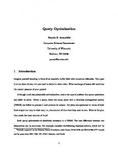
We have run preliminary experiments using the setup from Figure 2 (the shallows were flooded and the bridge’s gate was open). We have used the J-Sim (www.j-sim.org) simulation environment with a 20 by 20 rectangular WSN and 10 animals to be detected. We ran a query for 60 minutes, sampling at every minute. Our results are given in Figure 3. We have compared our approach with a base data collection mechanism where all the nodes wake-up at every minute and the nodes that sense an animal send a report to the base station. Our approach also used the same simple communication scheme. As expected, we see the number of sensor node activations drop by more than half while the communication for the two approaches remain the same. Depending on the number of sensors, animals to be detected, sampling frequency, duration of the query, and the application semantics, the benefits of our approach could change. However, we see that even with an expensive communication scheme, the number of activation savings can be an order of magnitude more that the number of transmissions in the system. Given the costs for starting up a node, sensing a stable input, computation and memory accesses–especially for elaborate acquisition schemes–the difference we observed could translate to major power savings for existing sensor platforms. Number of Transmissions
Number of Sensor Activations 2000
30000
25000
1600
20000 1200
15000 800
10000 400
5000
0
0
Our Approach
Base Approach
Our Approach
Base Approach
Figure 3. Experimental results
4
Figure 2. A dispersion with application semantics leading to a region of interest for our query. The simple graph model of the deployment is overlayed. The models used for acquisition can be probabilistic and come from previously sensed data. Administrators can also input non-probabilistic models into the system from the application domain, e.g., in our case we used maximum speed for animals as a simple pessimistic limit for dispersion. It is important to note that suppression-based methods can also directly be used with our work. Without using our approach, existing methods would have triggered a larger set of sensors. For example, [1, 2, 3] would have disseminated the query beyond the presented region of
Future Work
We are currently working on incorporating complex acquisition models into our framework. As future work, we plan to investigate update-based methods for addressing settings where domain facts can dynamically change their states. We also plan to incorporate some parts of the query plans into the broadcast packets so that the acquisition process can be guided incrementally and in a decentralized manner throughout the query lifetime. Finally, we plan to extend our experimental findings.
5
References
[1] A. Deshpande, C. Guestrin, S. Madden, J. M. Hellerstein, and W. Hong. Modeldriven data acquisition in sensor networks. In VLDB, pages 588–599, 2004. [2] S. Madden, M. J. Franklin, J. M. Hellerstein, and W. Hong. TinyDB: an acquisitional query processing system for sensor networks. ACM Trans. on Database Sys., 30(1):122–173, 2005. [3] A. Silberstein, R. Braynard, and J. Yang. Constraint chaining: on energy-efficient continuous monitoring in sensor networks. In SIGMOD, pages 157–168, 2006.