2. ( ) , where 1 and 2 are densities and is a smooth convex function. ⢠Includes KL and Renyi- divergences. ⢠Impor
Ensemble Estimation of Multivariate 𝑓-Divergence Kevin Moon, Alfred O. Hero III University of Michigan, Department of Electrical Engineering and Computer Science
Introduction
Application to Divergence Estimation
Proofs of Theorems 2 and 3
𝑓-divergence measures the difference between distributions
Setup: 𝑿1 , … , 𝑿𝑁 , 𝑿𝑁+1 , … , 𝑿𝑁+𝑀2 i.i.d. samples from 𝑓2 and 𝒀1 , … , 𝒀𝑀1 i.i.d. samples from 𝑓1 , 𝑇 = 𝑁 + 𝑀2 . Plug-in Estimators: the 𝑘-nn density estimate is
Principal tools are concentration inequalities and moment bounds applied to a higher order Taylor expansion of 𝐆𝑘 . Due to dependence of 𝐆𝑘 on the likelihood ratio, bounds on covariances of products of the density estimates are derived.
• Has the form G 𝑓1 , 𝑓2 =
𝑓1 𝑥 𝑓2 𝑥
𝑔
𝑓2 (𝑥) 𝑑𝑥, where 𝑓1 and 𝑓2 are
densities and 𝑔 is a smooth convex function • Includes KL and Renyi-𝛼 divergences • Important in statistics, machine learning, and information theory Convergence rates are unknown for most divergence estimators We derive the MSE convergence rates for kernel density plug-in 𝑓divergence estimators using 𝑘-nn kernel • Assume densities are smooth and two finite populations of i.i.d. samples are available
f i ,k ( X j )
Weighted Ensemble Estimation Let 𝑙 = 𝑙1 , … , 𝑙𝐿 be a set of index values and 𝑬𝑙 𝑙∈𝑙 be an ensemble of estimates of 𝐸. The weighted ensemble estimator is 𝑬𝑤 =
𝑤(𝑙)𝑬𝑙 , 𝑙∈𝑙
where 𝑙∈𝑙 𝑤 𝑙 = 1. Consider the following conditions on 𝑬𝑙 𝐶. 1 The bias is given by Bias(𝑬𝑙 ) =
𝑇 −𝑖/2𝑑
𝑐𝑖 𝜓𝑖 𝑙
+𝑂
𝑖∈𝐽
1 𝑇
: 𝑙∈𝑙
,
where 𝑐𝑖 are constants depending on the density, 𝐽 is a finite index set with length< 𝐿, min J > 0 and max 𝐽 ≤ 𝑑, 𝑑 is the dimension of the data, and 𝜓𝑖 𝑙 are basis functions depending only on the parameter 𝑙. 𝐶. 2 The variance is given by Var 𝑬𝑙 = 𝑐𝑣
,
Experiments
1 Gk N
f 1,k ( X i ) g . i 1 f 2,k ( X i )
Assumptions 1. 𝑓1 , 𝑓2 , and 𝑔 are smooth (𝑑 differentiable) 2. 𝑓1 and 𝑓2 have bounded support 3. 𝑓1 and 𝑓2 are strictly lower bounded 1/2 4. 𝑀1 = 𝑂 𝑀2 and 𝑘 = 𝑘0 𝑀2 MSE Convergence Rates: under the above assumptions, Theorem 2. The bias of the plug-in estimator 𝐆𝑘 is
Bias G k
𝑤
𝑠𝑢𝑏𝑗𝑒𝑐𝑡 𝑡𝑜
𝑤 𝑙 = 1, 𝑙∈𝑙
𝛾𝑤 𝑖 =
𝑤 𝑙 𝜓𝑖 (𝑙) = 0, 𝑖 ∈ 𝐽. 𝑙∈𝑙
We apply Theorem 1 to 𝑓 -divergence estimators to obtain the parametric rate of 𝑂 1/𝑇 . To do this, we verify conditions 𝐶. 1 and 𝐶. 2.
Truncated Gaussians, 𝑑 = 5
j d d k 1 k 1 O O o . k j 1 M 2 k M2
Theorem 3. The variance of the plug-in estimator 𝑮𝑘 is
Var G k
1 1 1 1 1 O 2 . o N M2 N M2 k
Truncated Gaussians, 𝑇 = 3000
Non-truncated Gaussians, d=5
Conclusions Derived MSE convergence rates for a plug-in estimator of 𝑓 divergence 1 Obtained an estimator with convergence rate of 𝑂 by applying 𝑇
the theory of optimally weighted ensemble estimation • Simple and performs well for higher dimension • Performs well for densities with unbounded support
where 𝑤0 is the solution to the following convex optimization problem: min 𝑤 2
Truncated Gaussian pdfs with different means and covariances Estimate Renyi-𝛼 divergence with 𝛼 = 0.8 for 100 trials Two experiments: Fixed 𝑑, increasing 𝑇; fixed 𝑇, increasing 𝑑
N
1 1 +𝑂 . 𝑇 𝑇
Theorem 1. [2] Under the conditions 𝐶. 1 and 𝐶. 2, there exists a weight vector 𝑤0 such that Ew E 2 O 1 , 0 T
M ic ( j) d i ,k
where 𝑘 ≤ 𝑀𝑖 , 𝑐 is the volume of a 𝑑-dimensional unit ball, and 𝑑 𝜌𝑖,𝑘 𝑗 is the distance to the 𝑘 th nearest neighbor of 𝑋𝑗 in 𝑌1 , … , 𝑌𝑀1 or 𝑋𝑁+1 , … , 𝑋𝑁+𝑀2 for 𝑖 = 1,2, respectively. The divergence estimate is
1 𝑇
We obtain an estimator with rate 𝑂 (𝑇 =sample size) by applying the theory of optimally weighted ensemble estimation • More computationally tractable than competing estimators
k
Acknowledgments Heat map of predicted bias of non-averaged 𝑓-divergence estimator based on Theorem 2 as a function of dimension and sample size.
Weighted Ensemble Divergence Estimator: Choose 𝐿 > 𝑑 − 1 and choose 𝑙 = 𝑙1 , … , 𝑙𝐿 . Let 𝑘 𝑙 = 𝑙 𝑀2 and 𝐆𝑤 = satisfies 𝑙∈𝑙 𝑤(𝑙)𝐆𝑘(𝑙) . From Theorem 2, the bias of 𝐆𝑘(𝑙) 𝑙∈𝑙
𝐶. 1 when 𝜓𝑖 𝑙 = 𝑙 𝑖/𝑑 and 𝐽 = 1, … , 𝑑 − 1 . From Theorem 3, the general form of the variance of 𝐆𝑘(𝑙) also follows 𝐶. 2. 𝑙∈𝑙
Theorem 1 then gives us the optimal weight to obtain a convergence rate of 𝑂 1/𝑇 .
This work was partially supported by NSF grant CCF-1217880 and a NSF Graduate Research Fellowship to the first author under Grant No. F031543.
References [1] K. Moon, A. Hero, “Ensemble estimation of multivariate 𝑓divergence,” Submitted to ISIT 2014. [2] K. Sricharan, D. Wei, and A. Hero, “Ensemble estimators for multivariate entropy estimation,” IEEE Trans. on Info. Theory, vol. 59, no. 7, pp 4374-4388, 2013.