Applications of Compressed Sensing in Communications ... - arXiv

1

Applications of Compressed Sensing in Communications Networks Hong Huang1 , Satyajayant Misra2 , Wei Tang1 , Hajar Barani1 , and Hussein Al-Azzawi1

arXiv:1305.3002v3 [cs.NI] 5 Feb 2014

1

Klipsch School of Electrical and Computer Engineering, New Mexico State University, NM, USA 2 Department of Computer Science, New Mexico State University, NM, USA

Abstract—This paper presents a tutorial for CS applications in communications networks. The Shannon’s sampling theorem states that to recover a signal, the sampling rate must be as least the Nyquist rate. Compressed sensing (CS) is based on the surprising fact that to recover a signal that is sparse in certain representations, one can sample at the rate far below the Nyquist rate. Since its inception in 2006, CS attracted much interest in the research community and found wide-ranging applications from astronomy, biology, communications, image and video processing, medicine, to radar. CS also found successful applications in communications networks. CS was applied in the detection and estimation of wireless signals, source coding, multi-access channels, data collection in sensor networks, and network monitoring, etc. In many cases, CS was shown to bring performance gains on the order of 10X. We believe this is just the beginning of CS applications in communications networks, and the future will see even more fruitful applications of CS in our field. Index Terms—Compressed sensing, communications networks, sensor networks.

I. I NTRODUCTION

P

ROCESSSING data is a big part of modern life. Interesting data typically is sparse in certain representations. An example is an image, which is sparse in, say, the wavelet representation. The conventional way to handle such signal is to acquire all the data first and then compress it, as is done in image processing. The problem with this kind of processing is, as Donoho puts it in his seminal paper [35]: ”Why go to so much effort to acquire all the data when most of what we get will be thrown away? Can we not just directly measure the part that will not end up being thrown away?” Indeed, compressed sensing (CS) does just that– measuring only the part of data that is not thrown away. The wellknown Shannon’s sampling theorem states that to recover a signal exactly, the sampling rate must be as least the Nyquist rate, which is twice the maximum frequency of the signal. In contrast, using CS, far fewer samples or measurements at far below the Nyquist rate are required to recover the signal as long as the signal is sparse and the measurement is incoherent, the exact meanings of which will be revealed later. In addition, CS has other attractive attributes, such as universality, faulttolerance, robustness to noise, graceful degradation, etc. Since its introduction in [10] and [35] in 2006, CS has received much attention in the research community. Thousands of papers have been published on topics related to CS, and hundreds of conferences, workshops and special sessions have

been devoted to CS [39]. CS has been showed to bring significant performance gains in wide-ranging applications from astronomy, biology, communications, image and video processing, medicine, to radar. Although there are good survey and tutorial papers on CS itself [3], [11], [14], [30], there is no good tutorial paper on the application of CS in communications networks to the best of the authors’ knowledge. We hope this paper will close the gap. Our intention is to enable the readers to implement their own CS applications after reading this tutorial. Therefore, instead of covering a wide-range of CS applications, we focus on a few representative applications and provide very detailed description for the covered applications. The intended readers should have some basic backgrounds in signal processing, communications networks in general, and sensor networks in particular. This paper contains a fair amount of mathematical formulas, since CS is a mathematical tool and mathematics is best expressed by formulas. Although CS has been applied in some areas of communications networks, we believe deeper and wider applications of CS in communications networks are plausible. Readers can use this tutorial to familiarize themselves with CS and seek a wider-range of fruitful applications. CS can be applied in various layers of communications networks. At the physical layer, CS can be used in detecting and estimating sparse physical signals such as ultra-wide-band (UWB) signals, wide-band cognitive radio signals, and MIMO signals. Also, CS can be used as erasure code. At the MAC layer, CS can be used to implement multi-access channels. At the network layer, CS can be used for data collection in wireless sensor networks, where the sensory signals are usually sparse in certain representations. At the application level, CS can be used to monitor the network itself, where network performance metrics are sparse in some transform domains. In many cases, CS was shown to bring performance gains on the order of 10X. We believe this is just the beginning of CS applications in communications networks, and the future will see even more fruitful applications of CS in our field. The rest of the paper is organized as follows. In Section II, we provide an overview of the CS theory. In Section III, we describe the algorithms that implement CS. In Section IV, we describe some variations of the CS theory. In section V, we provide a tutorial on CS applications in the physical layer. In Section VI, we described CS applications as erasure code and in the MAC layer. In section VII, we describe how CS is used in the network layer. In Section VIII, we describe CS

2

applications in the application layer. We conclude in Section IX.

of f suffices to recover the signal exactly, , where m n. Each measurement yj is a projection of the original signal, i.e., the m-dimensional measurement can be represented by

II. T HE T HEORY OF C OMPRESSED S ENSING The theory of CS was mostly established in [10] and [35], where the reader can find proofs of the results described below. A. Sparse Signal For the vector x = (xi ), i = 1, 2, ..., n its lp norm is defined by

n X kxkp = ( |x|p )1/p .

y = Φx

where y is the measurement vector and Φ is an m × n sensing matrix. Since m n, to recover x from y is an ill-posed inverse problem. In other words, there might be multiple x0 s that satisfy (6). However, we can take advantage of the fact that x is sparse in a certain representation Ψ, and formulate the following optimization problem:

(1)

(P0 )

i=1

The above definition applies to either row or column vector. Note that for p = 0, kxk0 is the number of nonzero elements in x; for p = 1, kxk1 is the summation of the absolute values of elements in x; for p = 2, kxk2 is usual Euclidean norm; and for p = ∞, kxk∞ is the maximum of the absolute values in x. We call a signal k-sparse if kxk0 ≤ k, namely x has only k nonzero elements. We also say the sparsity of the signal is k. In fact, few real-world signals are exactly k-sparse. Rather, they are compressible in the sense that they can be wellapproximated by a k-sparse signal. Denote Σk is the set of all k-sparse signals. The error incurred by approximating a compressible signal x by a k-sparse signal is given by σk (x)p = min kˆ x − xkp . x ˆ∈Σk

(2)

If x is k-sparse, σk (x)p = 0. Otherwise, the optimal k-sparse approximation of x is the vector that keeps the k largest elements of x with the rest elements setting to zero. Consider a compressible signal x and order its elements in descending order so that |x1 | ≥ |x2 | ≥ ... ≥ |xn |. We say the elements follow a power-law decay if |xi | ≤ ci−α

(3)

where c is a constant and α > 0 is the decay exponent. If x follows a power-law decay, there exist some constants c, α > 0, such that [31] σk (x)2 ≤ ck −α−1/2 .

(4)

In other words, the error also follows a power-law decay.

Although CS applies to both finite and infinite dimensional signals, we focus on finite dimensional signals here for the ease of exposition. Consider an n-dimensional signal f , which has a representation in some orthonormal basis Ψ = [ψ1 , ψ2 , ..., ψn ] where f=

n X

xi ψi = Ψx.

minkΨxk0 x

subject to y = Φx.

(5)

i=1

In the above, xi and ψi (a column vector) are the ith coefficient and ith basis, respectively. The CS theory says that if f is sparse in the basis Ψ, which needs not be known a priori, then, under certain conditions, taking m nonadaptive measurements

(7)

It is known that solving P0 is NP-hard. Fortunately, it was shown that one can replace the l0 norm by l1 norm, and formulate the following optimization problem instead as [9], [12], [34] (P1 )

minkΨxk1 x

subject to y = Φx.

(8)

It can be shown if the signal is sufficiently sparse, the solutions to P0 and P1 are the same [12]. P1 is a convex linearprogramming problem with efficient solution techniques. In the rest of the section, we will describe what kind of sensing matrix will enable signal recovery, and how many measurements are needed for the recovery. The most wellknown answers to the above questions are expressed in terms of spark, mutual coherence, and restricted isometry property. C. Spark The spark of a matrix Φ is the smallest number of columns of Φ that are linearly dependent [33]. To see why spark is relevant, consider the k-sparse solution to the linear equation y = Φx. The solution is not unique if there are two different k-sparse vectors x and x0 such that y = Φx = Φx0 , which implies Φ(x − x0 ) = 0. Equivalently, (x − x0 ) is in the null space of Φ. Since the sparsity of (x − x0 ) is at most 2k, so to ensure the uniqueness of the solution, the null space of Φ can not have vectors whose sparsity is less or equal to 2k. In other words, to guarantee the uniqueness of the k-sparse solution, the smallest number of linear dependent columns of Φ must be larger than 2k, or spark(Φ) > 2k.

B. The Basic Framework of CS

(6)

(9)

For the m × n matrix Φ, spark(Φ) ∈ [2, m + 1]. So, to make the solution unique, the number of measurements taken must satisfy m ≥ 2k. (10) It turns out that equation (9) is also the sufficient condition to guarantee the error bound given by [21] √ (11) kˆ x − xk2 ≤ cσk (x)1 / k where x and x ˆ are the original and the recovered signals, c is a constant, and σk (x)1 is defined in (2). So, if x is exactly k-sparse, then σk (x)1 = 0, and the signal recovery is exact.

3

D. Mutual Coherence Property (MIP) According to CS theory [32], to enable signal recovery, the sensing matrix Φ must be incoherent with the sparse representation Ψ. For the ease of exposition, we assume the column vectors of both matrices form ortho-bases of Rn , which is not required by CS theory. Formally, the mutual coherence between two matrices is defined by [33], [88] √ (12) µ(Φ, Ψ) = n max | hφk , ψj i | 1≤k,j≤n

where hφk , ψj i is the inner product of kth column in Φ and jth column in Ψ. In other words, the coherence measures the maximum correlation √ between the columns of Φ and Ψ, and it has a range of [1, n] [77], [83], [93]. The coherence is large when the two matrices are closely correlated, and is small otherwise. With probability 1 − δ, a k-sparse signal can be recovered exactly if m (the number of measurements) satisfies the following condition for some positive constant c [3], [13] m ≥ cµ2 (Φ, Ψ)k log(n).

(13)

Note that the number of measurements required increases linearly with the sparsity of the signal and quadratically with the coherence of the matrices. Note that the above MIP bound is not tight for some measurement matrices. E. Restricted Isometry Property (RIP) In CS, an important concept is the so-called restricted isometry property [8], [87]. We define the isometry constant δk of a matrix Φ as the smallest number such that the following holds for all k-sparse vectors x (1 − δk )kxk22 ≤ kΦxk22 ≤ (1 + δk )kxk22

(14)

Informally, we say a matrix Φ holds RIP of order k if δk is not too close to one. Three remarks follow: • A transformation of k-sparse signal by a matrix holding RIP approximately preserves the signal’s l2 norm. The degree of preservation is indicated by δk , with δk = 0 being exactly preserving and δk = 1 being not preserving. Because RIP preserves l2 norm, for a matrix Φ holding RIP, its null space does not contain k-sparse vector. As mentioned earlier, this is important because for any solution x of (8), x + x0 is also a solution, where x0 is a vector in the null space of Φ, making the solution not unique. RIP precludes such situation from arising. • RIP implies that all subsets of k columns of Φ are nearly orthogonal. • A further implication of RIP is that if δ2k is sufficiently small, then the measurement matrix Φ preserves the distance between any pair of k-sparse signals, i.e., (1 − δ2k )kx1 − x2 k22 ≤ kΦ(x1 − x2 )k22 ≤ (1 + δ2k )kx1 − x2 k22 . When the measurement involves noise, we can revise P1 by relaxing the measurement constraint as below (P2 )

minkΨxk1 x

subject to ky − Φxk2 ≤

(15)

where bounds the amount of noise. Using RIP, we can bound the error of signal recovery when noise is present. In fact, if

√ δ2k < 2 − 1, then for some constants c1 and c2 the solution x∗ to P2 satisfies [8], [87] kx − x∗ k2 ≤ c1

kx − xk k1 √ + c2 k

(16)

where xk is the vector x with all but the largest k elements set to zero. Two remarks follow: •

•

Consider the case where there is no noise. In such case, if x is k-sparse, i.e., x = xk , then the recovery is exact. On the other hand, if x is not k-sparse, then the recovery is as good as if we know beforehand the largest k elements and use them as an approximation. The contribution of the noise is a linear term. In other words, CS handles noise gracefully.

F. Relationships among Spark, MIP, and RIP Spark and MIP have the following relationship spark(Φ) ≥ 1 + 1/µ(Φ)

(17)

√ where µ(Φ) = µ(Φ, Φ)/ n. The above result is a straightforward application of the Gershgorin circle theorem [47]. RIP is strictly stronger than the spark condition. Specifically, if a matrix Φ satisfies the RIP of order 2k, then spark(Φ) ≥ 2k. RIP and MIP are related as follows. If Φ has unit-norm columns and coherence µ(Φ), then Φ satisfies the RIP of order k for all k < 1/µ(Φ). For general matrix, it is hard to verify whether the matrix satisfies the spark and RIP conditions. Verifying MIP is much easier, since it involves calculating the inner products between columns of two matrices and taking the maximum of products, referring to (12).

G. Measurement Matrices Random matrices are commonly used for measurement matrices, though non-random matrices can also be used as long as they satisfy spark, MIP, or RIP requirements. By definition, random matrices are those that have elements following independent identical distributions. Examples of random matrices include those, whose √ elements follow Bernoulli distribution (Prob(φi,j = ±1/ m) = 1/2) or Gaussian distribution with zero mean and variance of 1/m. With high probability, random matrices are incoherent with any fixed basis Ψ. Further, most random matrices obey the RIP and can serve as the measurement matrix Φm×n , as long as the following condition holds for some constant c that varies with the particular matrix used [29] m ≥ ck log (n/k).

(18)

In fact, using random matrices is near-optimal in the sense that it is impossible to recover signal using substantially fewer measurements than the left-hand side of (18).

4

TABLE I A LGORITHMS FOR IMPLEMENTING CS Algorithms Convex optimization algorithms [10], [26], [43], [51], [57] Greedy algorithms [37], [67], [70]–[72], [74], [76] Combinatorial Algorithms [23], [48], [62], [69]

III. T HE A LGORITHMS FOR I MPLEMENTING CS There are three main types of algorithms for implementing CS: convex optimization algorithms, combinatorial algorithms, and greedy algorithms. Convex optimization algorithms require fewer measurements but are more computationally complex than those of combinatorial algorithms. Those two types of algorithms represent two extremes in the spectra of the number of measurements and the computational complexity. Greedy algorithms provide a good compromise between the two extremes, which we provide more detailed descriptions below. Table (I) summarizes the computational complexity of various algorithms for implementing CS. A. Convex Optimization Algorithms With convex optimization algorithms, we use an unconstrained version of P2 given by the following 1 (19) min ky − Φxk22 + λkΨxk1 x 2 where λ can be selected based on how much weight we want to put on the fidelity to the measurements and the sparsity of the signal. Several ways to select λ were discussed in [40], [45]. Efficient algorithms exist to solve the convex optimization problem, such as basis pursuit [51], iterative thresholding that uses soft thresholding to set the coefficients of the signal [26], interior-point (IP) methods that uses the primal-dual approach [10], [57], and projected gradient methods that updates the coefficients of the signal in some preferred directions [6], [43]. (P4 )

B. Greedy Algorithms Greedy algorithms iteratively approximate the original signal and its support (the index set of nonzero elements). Earlier algorithms include Matching Pursuit (MP) [67], and its improved version Orthogonal Matching Pursuit (OMP) [74], [88], which is listed below as a representative greedy algorithm. In the algorithm listed above, we have set Ψ to identity matrix for the ease of exposition. In the algorithm, we iteratively select the column of Φ that is most correlated with current residual rj and add it to the current support Sj in step 7. Then, we update the current signal xj so that it is conforming to the measurements y and current support Sj . Finally, we update the current residual rj so that it contains measurements excluding those included by the current support. Denote Φj as the submatrix containing only columns in the current support Sj , then Pj = Φj (ΦTj Φj )−1 ΦTj . It can be shown that if the the signal x is sufficiently sparse, i.e., kxk0 < 12 (1 + µ(Φ)−1 ), OMP can exactly recover x when is set to zero [87]. For noisy

Computation complexity of the best algorithm in the category O(m2 n3/2 ) O(mn log k) O(k(log n)c ), where c is a positive constant.

Algorithm 1 OMP Algorithm Input: m × n measurement matrix Φ = (φi ), where φi is the ith column of Φ, n-dimensional initial signal x, and error threshold . 1: Output: approximate solution xj 2: Set j = 0 3: Set the initial solution x0 = 0 4: Set the initial residual r0 = y − Φx0 = y 5: Set the initial support S0 = ∅ 6: repeat 7: Set j = j + 1 8: Select index i so that maxkφTi rj k2 , update Sj = i Sj−1 ∪ i 9: Update xj = argminkφx − yk2 , subject to supp(x) = Sj

x

Update rj = (1 − Pj )y, where Pj denotes the projection onto the space spanned by the columns in Sj 11: until krj k2 ≤

10:

measurements, can be set to a nonzero value, for details of which the reader is referred to [74]. Compared with MP, OMP converges faster with no more than n iterations. Recent developments of this type of algorithms include the following. In [71], [72], regularized OMP (ROMP) is proposed that combines the speed and ease of implementation of the greedy algorithms with the strong performance guarantees of the convex optimization algorithms. In [70], a method called compressive sampling matching pursuit (CoSaMP) is proposed, which provides the same performance guarantee as that of the best optimization-based methods, and requires only matrix-vector multiplies. In [25], a subspace pursuit (SP) algorithm is proposed that has the same computational complexity as that of OMP but has the reconstruction accuracy on the same order as that of convex optimization algorithms. Both CoSaMP and SP incorporate ideas from convex optimization and combinatorial algorithms. In [37], Stagewise Orthogonal Matching Pursuit (StOMP) is proposed, which allows multiple coefficients of the signal to be added to the model in each iteration and performs a fixed number of iterations. In Algorithm 2, we present CoSaMP [70] as an example of the state-of-art greedy algorithm. The notation we use is the following. For signal x, let x(k) denote the signal that keeps the k largest components of x while setting the rest of the components to zero. For an index set T , let x|T denote the signal that keeps the components in T while setting the rest of the components to zero. Also, let ΦT denote the column sub-matrix of Φ whose columns are listed in T . Finally, let

5

A† = (AT A)−1 AT denote the pseudo-inverse of the matrix A. The CoSaMP algorithm consists of five major steps. 1) Identification: We form a signal proxy u from the current sample and identify the support Ω of the 2k largest components. 2) Support merger: We merge Ω with the support of the sparse signal in the previous round. 3) Estimation: We estimate the signal using the least-squares method to approximate the target signal on the merged support. 4) Pruning: We prune the resulting signal to be k-sparse. 5) Sample update: We update the sample z so that it reflects the residual r that contains the signal that has not been approximated. We stop when the halting criterion is met. There are three major approaches to halting the algorithm. In the first approach, we halt the algorithm after a fixed number of iterations. In the second approach, the halting condition is kzk2 ≤ 1 . In the third approach, we can use kuk∞ to bound the residual krk∞ , and require that krk∞ ≤ 2 . Using different approaches and parameters involve the tradeoff between approximation accuracy and computational complexity. Algorithm 2 CoSaMP Algorithm Input: m × n measurement matrix Φ, m-dimensional measurement y, sparsity level k. Output: approximate solution xj 1: Set j = 0 2: Set the initial solution x0 = 0 3: Set the current sample z = y 4: Set the initial support S = ∅ 5: repeat 6: Set j = j + 1 7: Form signal proxy u = ΦT z 8: Identify large signal components Ω = supp(u(2k) ) S 9: Merge supports S = Ω supp(xj−1 ) 10: Estimate signal using least-squares method x0|S = Φ†S y, x0|S c = 0 11: Prune the signal to obtain the next approximation xj = x0(k) 12: Update current sample z = y − Φxj 13: until halting criterion is true

C. Combinatorial Algorithms These algorithms were mostly developed by the theoretical computer science community, in many cases predating the compressed sensing literature. There are two major types of algorithms: group testing and data stream sketches. In group testing [48] [62], there are n items represented by an ndimensional vector x, of which there are k anomalous items we would like to identify. The values of elements of x are nonzero if they correspond to anomalous items and zero otherwise. The problem is to design a collection of tests, resulting in the measurement y = Φx, where the element of matrix φi,j indicates jth item is included in the ith test. The goal is to recover k-sparse vector x using the least number of tests, which is essentially a sparse signal recover problem in CS.

An example of data stream sketches [23], [69] is to identify the most frequent source or destination IP addresses passing through a network device. Let xi denote the number of times IP address i is encountered. The vector x is sparse since the network device is likely to see a small portion of IP address space. Directly storing xi is infeasible since the index set {i} is too large (232 , since IP address has 32 bits). Instead, we store a sketch defined by y = Φx, where Φ is an m×n-dimensional matrix with m n. Since y has a linear relationship with x, y is incrementally updated each time a packet arrives. The goal is to recover x from the sketch y, which again is a sparse signal recovery problem in CS.

IV. VARIATIONS OF CS In this section, we describe three variations to CS: 1) CS for multiple measurement vector signals, 2) CS for analogy signals, and 3) CS for matrix completion.

A. Multiple Measurement Vectors (MMV) Before proceeding further, we mention there is a method used in sensor networks that is related to MMV called distributed compressed sensing or joint sparse signal recovery. We will describe that method in Section VII.B of this paper. In MMV problems, we deal with l correlated sparse signals, which share the same support (the index set of nonzero coefficients). Instead of recovering each signal xi independently, we would like to recover the signals jointly by exploiting their common sparse support. Let X = (x1 , x2 , ...xl ) denote the n × l matrix representing the signals, and Λ = supp(X) denote the sparse support. The CS problem for MMV can be formulated as (P5 )

minkX|1 subject to Y = ΦX X

(20)

where Y is the m × l measurement matrix, In the above, we assume X is already in a sparse representation to simplify the presentation. It is straightforward to extend the results to the cases where X is not in a sparse representation. A necessary and sufficient condition to recover signal using CS is given by [28] spark(A) > 2|supp(X)| − rank(X) + 1.

(21)

Assume the signals are k sparse, then |supp(X)| = rank(X) = k. For an m × l matrix A, spark(A)≤ m + 1. So, the necessary and sufficient condition for signal recovery becomes m > k.

(22)

Recall that for a single measurement signal, the necessary and sufficient condition for signal recovery is m ≥ 2k, referring to (10). Thus MMV CS reduces the number of measurements by half compared with single measurement vector (SMV) CS.

6

pc (t) {−1, 1}

C. Matrix Completion

? x(t) -@ - Analog Filter @ h(t)

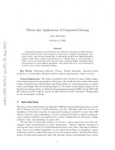
Fig. 1.

@ @

@ mM

y[m] -

Pseudo-random demodulation for AIC.

B. Analog-to-Information Conversion (AIC) Today, digital signal processing is prevalent. Analog-todigital converters (ADC) are used to convert analog signals to digital signals. ADC requires sampling at Nyquist rate. The ever-pressing demands from applications, such as ultra-wideband communications and radar signal detection, are pushing the performance of ADCs toward their physical limits. In [58], [60], [68], CS was used to implement an analog-to-information converter. AIC was shown to be particularly effective for wideband signals that are sparse in frequency domain. We provide an overview of AIC below. Assume analog sign x(t) is sparse in an orthogonal basis (Ψ = {ψ1 (t), ψ2 (t)..., ψn (t)}) and is expressed by x(t) =

n X

θi ψi (t).

(23)

i=1

AIC is composed of three components, a wide-band pseudorandom signal demolulator pc (t), a filter h(t) (typically a lowpass filter), and a low-rate analog-to-digital converter (ADC), referring to Figure 1. The input of AIC is the signal x(t). The output is the low-rate measurement yi , given by Z ∞ yi = x(τ )pc (τ )h(t − τ ) dτ |t=m∆ (24) −∞

where ∆ is the sampling period. Substituting (23) into (24), we have Z ∞ n X yi = θj ψj (τ )pc (τ )h(i∆ − τ ) dτ. (25)

For matrix completion to be possible, we need to impose the following condition on M . Let the singular value decomposition (SVD) of M be X M= σk uk vk∗ (29) k

where σ1 ≥ σ2 ≥ ... ≥ σr are the singular values, and u1 , u2 , ..., ur ∈ Rn1 and v1 , v2 , ..., vr ∈ Rn2 are singular vectors. The condition we impose is as follows p p (30) kuk k∞ ≤ µB /n1 , kvk k∞ ≤ µB /n2 . for some µB ≥ 1, where kxk∞ = maxi |xi |. In other words, we impose the condition that the singular vectors are not spiky and are sufficiently spread. In principal, we can recover the matrix by solving the following minimization problem min rank(X) subject to PΩ (X) = PΩ (M ).

(31)

−∞

j=1

The equivalent measurement matrix is given by Z ∞ φi,j = ψj (τ )pc (τ )h(i∆ − τ ) dτ.

However, the above problem is NP-hard [18]. An alternative is the convex relaxation as follows [15], [16]. (26)

−∞

So the compressed sensing with analog signals can be formulated as (P3 )

In matrix completion [15], [16], [55], [56], we seek to recover a low-rank matrix from a small, noisy sample of its elements. Matrix completion has a wide range of applications in collaborative filtering, machine learning, control, remote sensing, computer vision, etc. We first describe the notations used in this subsection. Let X ∈ Rn1 ×n2 denote the matrix of interest with singular values {σk }. Let kXk∗ denote the nuclear norm, which is the l1 norm of the singular value vector. We assume that the samples are randomly selected without replacement, and there is no row and column that is not sampled, since in such case the matrix completion is impossible. In the following, we first describe exact matrix completion [15], [55], and then briefly cover noisy matrix completion [16], [56]. Suppose M ∈ Rn1 ×n2 is the matrix we want to complete, and we have a small, exact sample of its elements Mi,j , (i, j) ∈ Ω, where Ω is a subset of indices of M . The sampling operator PΩ is given by ( Xi,j if (i, j) ∈ Ω [PΩ ]i,j = (28) 0 otherwise.

minkθk1 θ

subject to y = Φθ

(27)

which is exactly the same formulation as P1 with Ψ set to identity matrix and the x vector replaced by the θ vector. In [60], simulation was performed using a 200 MHz carrier modulated by a 100 MHz signal. AIC was shown to be able to successfully recover the signal at a sampling rate of one sixth of the Nyquist rate.

min kXk∗

subject to PΩ (X) = PΩ (M ).

(32)

The above nuclear-norm minimization is the tightest convex relaxation of the rank minimization problem [15], [16]. Let M ∈ Rn1 ×n2 denote a matrix of rank r = O(1) obeying . (30), and n = max(n1 , n2 ). We observe m elements of M with indices uniformly randomly sampled. In [16], it is shown that for a constant c, if the following condition is satisfied m ≥ cµ4B nlog2 n

(33)

then M is the unique solution to (32) with probability of at least 1 − n−3 . In other words, with high probability, nuclearnorm minimization can perform matrix completion without error, using a sample set of size O(nlog2 n). In addition, if we

7

scale the constant in (33) as c = cβ, the success probability becomes 1 − nβ . An n1 × n2 matrix with rank r has r(n1 + n2 − r) degrees of freedom (DoF), which is equal to the number of parameters in the SVD. When r is small, the DoF is much smaller than n1 n2 , which is the total number of elements in the matrix. The nuclear-norm minimization can recover the matrix using a sample size that exceeds the DoF by a logarithmic factor. To recover the matrix, each row and column must be sampled at least once. It is well know that this occurs when the sample size is of O(nlogn), since it is the same as the coupon collector’s problem. Thus, (33) misses the information theoretic limit by a logarithmic factor. For matrices with all values of the rank, the condition for matrix completion is that the matrix must satisfy the strong incoherence property with a parameter µ, the definition of which is somewhat involved and we refer the reader to the reference [16]. Many matrices obey the strong incoherence property, such as matrices that obey (30) with µB = O(1), with very few exceptions. Let M ∈ Rn1 ×n2 denote a matrix of arbitrary rank r . obeying strong incoherence with parameter µ, and n = max(n1 , n2 ). We observe m elements of M with indices uniformly randomly sampled. In [16], it is shown that for a constant c if the following condition is satisfied m ≥ cµ2 nrlog6 n

(34)

then M is the unique solution to (32) with probability of at least 1 − n−3 . In other words, if the matrix is strongly incoherent, with high probability, nuclear-norm minimization can perform matrix completion without error using a sample set of size exceeding the DoF by a logarithmic factor. In real-world applications, samples always contain noise. Thus, our observation model is given by Yi,j = Mi,j + Zi,j or PΩ (Y ) = PΩ (M ) + PΩ (Z)

(35)

where Zi,j is the noise. We assume that kPΩ (Y )kF ≤ δ for some δ > 0. For instance, if {Zi,j } is a√white noise with standard deviation of σ, then δ 2 ≤ (m + 2 2m)σ 2 with high probability [16]. To complete the matrix M , we solve the following minimization problem min kXk∗

subject to kPΩ (X − Y )kF ≤ δ.

(36)

In words, we seek the matrix that has the minimum nuclearnorm and is consistent with the data. The above minimization problem can be solved by the FPC algorithm [66] as follows 1 kPΩ (X − Y )k2F + λkXk∗ (37) 2 for some positive constant of λ. We refer the reader to [16], [56] for details. min

V. A PPLICATIONS OF CS IN THE P HYSICAL L AYER CS can be used in detecting and estimating sparse physical signals, such as MIMO signals, wide-band cognitive radio signals, and ultra-wide-band (UWB) signals, etc. The details are provided below.

A. MIMO Signals Channel state information (CSI) is essential for coherent communication over multi-antenna (MIMO) channels. Convention holds that the MIMO channel exhibits rich multi-path behavior and the number of degrees of freedom is proportional to the dimension of the signal space. However, in practice, the impulse responses of MIMO channel actually are dominated by a relatively small number of dominant paths. This is especially true with large bandwidth, long signaling duration, or large number of antennas [24], [89]. Because of this sparsity in the multi-path signals, CS can be used to improve the performance in channel estimation. Consider a MIMO channel with NT transmitters and NR receivers. Assume that channel has two-sided bandwidth of W and the signaling has a duration of T . Let s(t) denote the NT dimensional transmitted signal, s˜(f ) its element-wise Fourier transform, h(t, f ) the time-varying frequency response matrix, which has a dimension of NR × NT . Without the noise, the received signal is given by [2] Z w/2 x(t) = h(t, f )˜ s(f )ej2πf t df. (38) −W/2

For a multi-path channel, the frequency response is the summation of the contributions from all the paths h(t, f ) =

NP X

j2πνn t j2πτn f βn aR (θR,n )aH e T (θT,n )e

(39)

n=1

where NP denotes the number of paths. For path n, βn denotes the complex path gain, θR,n the angle of arrival (AoA) at the receiver, θT,n the angle of departure (AoD) at the transmitter, νn the Doppler shift, and τn the relative delay. The NR dimensional vector aR (θR,n ) is array response vector at the receiver. The NT -dimensional vector aT (θT,n ) is array steering vector at the transmitter, and the superscript H denotes matrix conjugate transpose. We assume that the maximum delay is τmax , then τ ∈ [0, τmax ]. Also, the two-sided Doppler spread is in the range ν ∈ [−νmax /2, νmax /2]. The maximum antenna angular spread is assumed at the critical antenna spacing (d = λ/2), thus (θR,n , θT,n ) ∈ [−1/2, 1/2] × [−1/2, 1/2] in the normalized unit. It is also assumed that the channel is both time-selective (T νmax ≤ 1) and frequency-selective (W τmax ≤ 1). The physical model expressed by (39) is nonlinear and hard to analyze. However, it can be wellapproximated by a linear model known as a virtual channel model [80], [81]. The virtual model approximates the physical model by uniformly sampling the physical parameter space [βn , θR,n , θT,n , τn , νn ] at a resolution of (∆θR,n , ∆θT,n , ∆τn , ∆νn ) = (1/NR , 1/NT , 1/W, 1/T ). The approximate channel response is given by h(t, f ) '

NR X NT L−1 M X X X

hv (i, k, l, m)

i=1 k=1 l=0 m=−M m

l

j2π T t j2π W f e aR (i/NR )aH T (k/NT )e X hv (i, k, l, m) ' βn n∈[sampling point]

(40) (41)

8

where the summation in (41) is over all paths that contribute to the sampling point, and a phase and attenuation factor has been absorbed in βn . In (40), NR , NT , L = dW τmax e+1, and M = dT νmax /2e denote the maximum numbers of resolvable AoAs, AoDs, delays, and one-sided Doppler shifts. Basically, the virtual model characterizes the physical channel using the matrix hv , which has a dimension of D = NR × NT × L × (2M + 1). For sparse MIMO channels, the number of nonzero elements d in the matrix hv is far fewer than D. We call such channel d-sparse. Since the virtual model is linear, we can express the received training signal as

1) Spectrum Sensing: A Digital Approach: In this approach, the signal is first converted to the digital domain, and then CS is performed on the digital signal. Let x(t) denote the signal sensed by CR, B the frequency range of the wide-band, F the set of frequency bands currently used by other users. Typically, |F | B [79], indicating that x(t) is sparse in the frequency domain and thus CS is applicable. So, instead of sampling at Nyquist rate fN , we can sample at a much slower rate roughly around |F |fN /B. In [85], the CS formulation of spectrum sensing was proposed as

ytr = ΦHv

where f is signal representation in the frequency domain, F −1 is the inverse Fourier transformation, and S is a reduced-rate sampling matrix operating at a rate close to |F |fN /B, and xt is the reduced rate measurement. Simulation results show that good signal recovery can be achieved at 50% Nyquist rate [79]. 2) Spectrum Sensing: An Analog Approach: In this approach, CS is directly performed on the analog signal [90], which has the advantage of saving the ADC resources, especially in cases where the sampling rate is high. The implementation is similar to that described in Section IV-B. A parallel bank of filters are used to acquire measurements yi . To reduce the number of filers required, which is equal to the number of measurements M and can be potentially large, each filter samples time-windowed segments of signal. Let NF denote the number of filters required, and NS denote the number of segments each filter acquires. As long as NF NS = M , the measurement is sufficient. Simulations were performed for an OFDM-based CR system with 256 sub-carriers where only 10 carriers are simultaneously active. The results showed that a CS system with 8-10 filters can perform spectrum sensing at 20/256 of the Nyquist rate [90]. 3) Spectrum Sensing: A Cooperative Approach: The performance of CS-based spectrum sensing can be negatively impacted by the channel fading and the noise. To overcome such problems, a cooperative spectrum sensing scheme based on CS was proposed in [86]. In this scheme, the assumptions are that there are J CRs and I active primary users. The entire frequency range is divided into F non-overlapping narrowbands {Bi }F i=1 . In the sensing period, all CRs remain silent and cooperatively perform spectrum sensing. The received signal at jth CR is

(42)

where Hv is a D-dimensional column vector that contains all the elements in hv , ordered according to the index set (i, k, l, m), and Φ is an M × D-dimensional measurement matrix, which is a function of transmitted training signal and array steering and response vectors. We can formulate a CS problem as follows Hv = arg minkHv k1

subject to ytr = ΦHv .

(43)

Hv

The requirement for the measurement is that it is a uniformly random sampling of the signal in the domain of (i, k, l, m). It is shown in [2] that with high probability of success, roughly d instead of D measurements are enough to recover the D-dimensional channel vector Hv , which provides significant savings in training resources consumed, especially for sparse-MIMO channels. The details are given in [2]. Similar results are also reported in [53], [84] for RF signals and in [4] for underwater acoustic signals.

B. Wide-Band Cognitive Radio Signals Dynamic spectrum access (DSA) is an emerging approach to solve today’s radio spectrum scarcity problem. Key to DSA is the cognitive radio (CR) that can sense the environment and adjust its transmitting behavior accordingly to not cause interference to other primary users of the frequency. Thus, spectrum sensing is a critical function of CR. However, wideband spectrum sensing faces hard challenges. There are two major approaches to do wide-band spectrum sensing. First, we can use a bank of tunable narrow-band filters to search narrow-bands one by one. The challenge with this approach is that a large number of filters need to be used, leading to high hardware cost and complexity. Second, we can use a single RF front-end and use DSP to search the narrow-bands. The challenge in this approach is that very high sampling rate and processing speed are required for wide-band signals. CS can be used to overcome the challenges mentioned above. Today, a small portion of the wireless spectrum is heavily used while the rest is partially or rarely used fcc2002. Thus, the spectrum signal is sparse and CS is applicable. In this subsection, we introduce three approaches of applying CS to the spectrum sensing problem.

f = arg minkf k1 subject to xt = Sx(t) = SF −1 f

(44)

f

xj (t) =

I X

hi,j (t) ∗ si (t) + nj (t)

(45)

i=1

where hi,j is the channel impulse response, si (t) is the transmitted signal from primary user i, ∗ denotes convolution, and nj (t) denotes noise at the receiver j. We take discrete Fourier transform on xj (t) and obtain x ˜j (f ) =

I X

˜ i,j (f )˜ h si (f ) + n ˜ j (f ).

(46)

i=1

In this scheme, spectrum detection is possible even when the channel impulse responses are unknown. If x ˜j (f ) 6= 0, then

9

some primary user is using the channel unless the channel suffers from deep fades. Since it is unlikely that all the CR suffer from deep fades at the same time, cooperative spectrum sensing is much more robust than individual sensing. Cooperative spectrum sensing is carried out in two steps. In the first step, compressed spectrum sensing is carried out at each individual CR using the approach in [85]. In addition, the jth CR maintains a binary F -dimensional occupation vector uj , where uj,i = 1 if the frequency band is sensed to be occupied and ui = 0 otherwise. In the second step, CRs in the one-hop neighborhood exchange the occupation vectors and then update their own occupation vectors using the technique of average consensus [91] as follows X wj,k (uk (t) − uj (t)) (47) uj (t + 1) = uj (t) + k∈Nj

where Nj is the neighborhood of jth CR, and wj,k is the weight associated with edge (j, k), the selection rules of which are described in [91]. With proper selection rules, it can be shown that J 1X uk (0). (48) lim uj (t) = t→∞ J k=1

In other words, the frequency occupation vectors of the CRs in the neighborhood all reach the same value that is the average of their initial values. The jth CR can decide the frequency band i is occupied if uj,i ≥ 1/J, or a majority rule can be used, i.e., the frequency band i is considered occupied if uj,i ≥ 1/2. Simulation results showed that the spectrum sensing performance improves with the number of CRs involved in the cooperative sensing and the average consensus converges fast (in a few iterations) [85].

where p(t) is the ultra-short pulse used to carry information, and h(t) is the impulse response of the UWB channel. Typically a Gaussian pulse or its derivatives can be used as UWB 2 2 pulse, i.e., p(t) = pn (t)e−t /2σ , where pn (t) is a polynomial of degree n, and σ represents the width of the signal. The impulse response of the channel can be expressed as h(t) =

L X

θi δ(t − τi )

(50)

i=1

where δ() is the Dirac delta function, θi and τi are the gain and the delay of the ith-path received signal, and L is the total number of propagation paths. Typically, the number of the channel parameters (θi and τi ) is on the order of 103 . However, most of the paths carry negligible energy and can be ignored. In other words, the channel parameters are sparse and CS can be used to estimate them. Two approaches were proposed in [73] for UWB channel estimation using CS. One is correlator-based and the other is rake-receiver-based. It was shown that CSbased approaches outperform the traditional detector using only 30% of ADC resources. 2) UWB Echo Signal Detecion: In reference [82], the authors proposed to use CS to detect UWB radar echo signals. Let s(t) denote the transmitted signal and τ as the Nyquist sampling interval of the echo signal. All time-shifted versions of s(t) constitute a redundant dictionary as follows Ψ = {ψi (t) = s(t − iτ ), i ∈ [1, 2, ..., n]}.

(51)

The received signal is sparse in such dictionary and can be expressed as k X θi ψi (t) (52) x(t) = i=1

C. Ultra-Wide-Band (UWB) Signals UWB communications is a promising technology for lowpower, high-bandwidth wireless communications. In UWB, an ultra-short pulse, on the order of nanoseconds, is used as the elementary signal to carry information. The advantages of UWB are: 1) The implementation of the transmitter is simple because of the use of base-band signaling. 2) UWB has little impact on other narrow-band signals on the same frequency range, since its power spreads out on the broad frequency range. However, one of the challenges for UWB is that it requires extremely high sampling rate (several GHz) to digitize UWB signals based on the Nyquist rate, leading to high cost in hardware. Since UWB signals are sparse in the time domain [73], we can apply CS, which provides an effective solution to this problem by requiring much lower sampling rate. There are a number of recent papers in this area, and we provide two examples below. 1) UWB Channel Estimation: In reference [73], CS was applied to UWB multi-path channel estimation. The received multi-path UWB signal can be expressed as x(t) = p(t) ∗ h(t) =

L X i=1

θi p(t − τi )

(49)

where k is the number of target echoes and represents the sparsity of the signal, and θi indicates the amplitude of ith target echo. Equation (52) has the exact same form as (23) and standard methods of CS can be used to detect the UWB echo signals. It was shown in [82] that the sampling rate can be reduced to only about 10% of the Nyquist rate. VI. CS A PPLICATIONS AS E RASURE C ODE AND IN THE MAC L AYER In the following, we describe CS applications as erasure code and in the MAC layer. A. CS as Erasure Code Many physical phenomena are compressible or sparse in some domains. For example, virtual images are sparse in the wavelet domain and sound signals are sparse in the frequency domain. The conventional approach is to use source coding to compress the signal first, and then use erasure coding for protection against the missing data caused by the noisy wireless channel. Let x denote the n-dimensional signal. Let S and E denote the m × n source coding matrix and l × m erasure coding matrix, respectively. If the signal is k-sparse in some domain, m is close to k. If the expected probability

10

of missing data is p, then l = m/(1 − p). The transmitted signal is ESx, and the received signal is CESx, where the linear operator C models the channel. C is a sub-matrix of the identity matrix Il with e rows deleted, e being the number of erasures. If e ≤ l − m, the decoding at the receiver will be successful; otherwise the data can not be decoded and is discarded. CS can be used as an effective erasure coding method. In [17], CS was applied in wireless sensor networks as erasure code. At the source l measurements of the signal are generated by random projections y = Φx and sent out, where Φ is a l × n-dimensional random matrix. The received signal is y 0 = Cy, with e measurements erased. Suppose each measurement carries its serial number, we know where the erasure occurred and therefore the matrix C. At the receiver, the standard CS procedure is carried out x = arg minkΨxk1 subject to y 0 = CΦx.

(53)

x

where Ψ is the representation, under which x is sparse. Since erasure occurs randomly, CΦ is still a random matrix. CS performs data compression and erasure coding in one stroke. Information about the signal is spread out among l measurements, of which m measurements are expected to be correctly received, with m on the same order of k, the sparsity of the data. Compared with conventional erasure coding methods, CS has similar compression performance but two outstanding advantages: 1) CS allows graceful degradation of the reconstruction error when the amount of missing data exceeds the designed redundancy, whereas the conventional coding methods do not. Specifically, if e ≤ l − m, conventional decoding can not recover the data at all. However, if RIP holds, according to (16), CS can still recover partial data, with an error no larger than that of the approximate signal, which keeps the largest l−e elements of the sparse signal and sets the rest of the elements to zero. 2) In terms of energy consumed in the processing, performing CS erasure coding is 2.5 times better than performing local source coding and 3 times better than sending raw samples [17]. B. CS in On-Off Random Access Channels In [46], a connection was made between CS and on-off random access channels. In an on-off random multiple access channel, there are N users communicating simultaneously to a single receiver through a channel with n degrees of freedom. Each user transmits with probability λ. Typically, λN < n N . User i is assigned as codeword an n-dimensional vector φi . The signal at the receiver from user i is φi xi , where xi is a nonzero complex scalar if the user is active and zero otherwise. The total signal at the receiver is given by y=

N X

φi xi + w = Φx + w

(54)

i=1

where w is the noise, x = [x1 , x2 , ..., xN ], and Φ = [φ1 , φ2 , ...φN ] is the codebook. The active user set is defined by Ω = {i : xi 6= 0}. (55)

The goal of the receiver is to estimate Ω. Since |Ω| n, we have a sparse signal detection problem. A formulation in terms of CS is as follows x ˆ = arg min µkxk1 + ky − Φxk22

(56)

x

where µ > 0 is an algorithm parameter that weights the importance of sparsity in x ˆ. It was shown in [46] that the CS-based algorithms perform better than single-user detection in terms of the number of measurements required to recover the signal, and have some near-far resistance. At high signal-to-noise ratio (SNR), CSbased algorithms perform worse than the optimal maximum likelihood detection. However, CS-based algorithms are computationally efficient, whereas the optimal maximum likelihood detection is not computationally feasible. VII. A PPLICATIONS OF CS IN THE N ETWORK L AYER As mentioned before, most natural phenomena are sparse in some domains, and CS could be effective in wireless sensor networks (WSN) that monitor such phenomena. In [1], CS was used to gather data in a single-hop WSN. Sensors transmit random projections of their data simultaneously in a phase-synchronized channel. The base station receives the summation of the randomly projected data, which constitutes a CS measurement. The l1 -norm minimization is performed at the base station to recover the sensory data. An overview of CS’ potential applications in WSN was provided in [52]. In the following, we provide a few detailed examples. We first present a representative CS-based sensory data collection scheme and then present three approaches to reduce the measurement costs: 1) using the joint-sparsity in data to reduce the number of measurements, 2) using sparse random projection to reduce number of measurements, and 3) using data routing to reduce the cost of data transport. We compare the performance of various data collection schemes at the end of the section. A. Compressive Data Gathering (CDG) in WSN In [64], CS was used for data collection in WSN. In the following, we describe the proposed data collection scheme, and how it handles the abnormal sensor readings. 1) The CS-Based Data Collection Scheme: Consider a large-scale sensor network with n nodes, each of which holds a value xi . Assume that a shortest-path spanning tree rooted at the base station is built, and that the base station and sensors agree to the seeds for random number generation. To collect the data, m measurements are taken. For measurement j, the data transmissions start from the leaf-nodes of the spanning tree and work in rounds. In each round, the children send their data to the parent in the tree. Specifically, in the jth round, each leaf-node sends the random projection of its data (yj,i = φj,i xi ) to its parent in the tree. The parent node l collects data sent by all its children and compute an partial measurement as follows X yj,l = yj,i + φj,l xl (57) i∈Nl

11

where Nl denotes the children of node l. The parent node in turn sends its partial measurement to its own parent. This continues until the base station receives the partial measurements from its Pnchildren and compute the complete measurement yj = i=1 φj,i xi . An example is given in Figure 2, where :rZ r ~ Zr r r sr > Q r Z Zr r r rH ~ > S j H r + r r w r-9 S r ? / r r r S o ? YHr Sr dy H XX? r / r-rXz * r 6 r rX * r r 9 r O C r rz X r : k Q 9 r X r Qr CO 6 CO Cr r CrX r yXr r9

Fig. 2.

nk 1

} > Z Z Z k n6 nk 2 nk 3 J ] J BM J B nk 8 B nk nk 4 7 nk 5

the data gathering tree is shown on the left and a portion of the tree is magnified on the right. At the jth round, Node 4 and 5 send their data φj,4 x4 and φj,5 x5 to node 3. Node 3 computes the partial measurement φj,3 x3 + φj,4 x4 + φj,5 x5 , and sends it to node 1. Similar procedure is performed for other nodes. The base station is able to recover the data by solving the CS problem below subject to

ky − Φxk2 <

(58)

x

where Ψ is the basis under which the data is sparse, and is the error tolerance. Using convention methods, the energy consumption in data transmission is very unevenly distributed. The children of the base station are responsible to relaying O(n) pieces of data, causing them to die quickly due to battery depletion. On the other hand, in CDG each node transmit exactly m times, and the energy consumption is perfectly balanced. One shortcoming of CDG is that the nodes close to the leaves of the network are required to send more pieces of data than that of the conventional method. A leaf-node is required to send one piece of data (its own sensory reading) in the conventional method, but with CS it is required to send m pieces of data. To solve this problem, a hybrid CS scheme was proposed, where if a node sends less than m pieces of data in the conventional method, the conventional method is used, otherwise CS is used [65]. 2) Data Recovery with Abnormal Readings: CS can also be used to recover data with abnormal readings. For example, if a signal is smooth in the time domain, then its representation in the Fourier domain is sparse. If spikes are injected into the time domain signal, then the signal’s representation in the frequency domain is no longer sparse. However, we can decompose the signal into two parts x = x0 + x1

x = arg minkΨx0 + Ix1 k1

subject toky − Φxk2 < (60)

x

Data collection tree in CDG.

x = arg minkΨxk1

where x0 and x1 represent normal and abnormal parts, respectively. Since the spikes are sparse in the time domain and the normal signal is sparse in the frequency domain, the l1 -norm minimization is altered to

(59)

where Ψ is the Fourier transformation matrix and I is the identity matrix. A representation like Ψx0 + Ix1 is called an over-complete representation. Donoho et al. showed it is feasible to achieve stable recovery of the signal in overcomplete representations [36].

B. Distributed Compressed Sensing (DCS) in WSN Consider a WSN monitoring a natural phenomenon. Among the signals obtained by the sensors, there are likely both intra-signal and inter-signal correlations. Leveraging these correlations, DCS uses the joint sparsity of the signals to reduce the number of measurements for signal recovery [5], [38], in a fashion similar to MMV described in Section IV.A, but with some differences in problem formulation. DCS requires no collaboration among the sensors, and provides universal encoder for any jointly sparse signal ensemble. In the following, we first introduce three joint sparsity models and then describe signal recovery algorithms. 1) Joint Sparsity Models (JSM): Assume the signals obtained by the sensors are xj , j = 1, 2, ...J, and they are sparse in basis Ψ. JSM1: In this model, each signal is composed of a common sparse part and an individual sparse part as follows xj = z0 + zj

with z0 = Ψθ0 , zj = Ψθj

(61)

where the coefficients θ0 and θj are k0 and kj -sparse, respectively. An example of this model is the temperature signals, which can be decomposed into a global average value plus a value reflecting local variations. JSM2: In this model, all signals share the same index set of nonzero coefficients in the sparse representation, and different signals have different individual coefficients as follows xj = Ψθj

(62)

where the coefficients θj are k-sparse. An example of this model is the image observed by multiple sensors, which has the same sparse wavelet-representation but each sensor senses a different value due to different levels of phase-shift and attenuation. JSM3: This model is an extension of JSM1 in that the common part is no longer sparse in any basis xj = z0 + zj

with z0 = Ψθ0 , zj = Ψθj

(63)

where the coefficients θj are kj -sparse. An example of this model is the signals detected by sensors in the presence of strong noise, which is not sparse in any representation.

12

2) Joint Reconstruction: To reconstruct the signal, sensor j acquires its n-dimensional signal xj , takes random projections of the signal yj = Φj xj , where Φj is the mj × n-dimensional measurement matrix, and sends yj to the base station. After receiving the measurements from all the sensors, the base station starts the reconstruction, which is different for each of the sparsity models and is described separately below. JSM1: To recover the signal, the following linear program is sovled [θ0 , θ1 , θ2 , ...θJ ] = arg min

J X

kθj k1

θ0 ,θ1 ,θ2 ,...θJ j=0

subject to yj = ΦΨθj

∀j = 0, 1, 2, ..., J.

(64)

JSM2: In this model, conventional greedy pursuit algorithms (such as OMP) are modified. Specificly, step 7 in Algorithm 1 is modified so that the index set inserted to Sj includes only the indices of the common support, i.e., the nonzero items having the same indices among all sensors. JSM3: In this model, each sensor’s signal is the addition of a common part z0 that is not sparse and a sparse signal zj called innovation. The alternating common and innovation estimation (ACIE) scheme was proposed to recover signals [38]. ACIE alternates between two steps: 1) Estimate z0 by treating zj as noise that can be averaged out. 2) Estimate zj by subtracting z0 from the signal and using conventional CS recovery techniques. Extensive simulations have been carried out that demonstrate CS leveraging joint sparsity models can significantly reduce the number of measurements required. For detail, the reader is referred to [5]. C. Sparse Random Projection (SRP) in WSN The measurement matrix Φ used in conventual CS is dense in the sense that there are few zero elements in each row of Φ. This means each measurement requires data from O(n) sensors, which is expensive to acquire. Fortunately, it was shown in [92] that sparse random projections (SRP) can be used to reduce the cost of measurement, where the measurement matrix is given by  with prob. p = 1/2s  +1 −1 with prob. p = 1/2s φj,i = (65)  0 with prob. p = 1 − 1/s where s is a parameter that determines the sparseness of the measurement. In other words, SRP requires data from only O(n/s) instead of O(n) sensors. In order to recover a k-sparse signal with high probability, i.e. with probability 1 − n−γ for some positive γ, the number of measurements required is given by m = O(sM 2 k 2 log n) (66) where M is the peak-to-total energy ratio and is given by M≡

kxk∞ . kxk2

(67)

M bounds the largest element of the signal. SRP works well only if the signal is not too concentrated in a few elements.

A distributed algorithm for data collection in WSN was proposed in [92], which works in two steps. In the first step, assuming the base station and sensors agree to the seeds for random number generation, each sensor i generates a random projection φj,i xi . If φj,i is zero, nothing needs to be done, otherwise the sensor sends the random projection to another sensor chosen randomly, referring to Figure 3. Since Φ is ssparse, each sensor sends n/s pieces of data. In the second step, sensor j waits until it receives n/s pieces of data and then Pn/s computes a measurement yj = i=1 φj,i xi . The base station sends query to m sensors, and gets m measurements back. As long as m satisfies (66), the signal is recovered successfully with high probability. i

y

i QQ s i y i : S o y S S Sy i y y Q

i

Fig. 3. SRP: the node in the center receives data from a randomly selected subset of nodes (dark ones) in the network.

There is a tradeoff involved in SRP. The larger the value of s, the less the cost of data spreading among the sensors, but the higher the cost of the query from the base station. Suppose the average number of hops between two nodes is h. The data spreading in SRP requires hn2 /s transmissions. The data query requires O(hsM 2 k 2 log n) transmissions. The optimum value of s is given by n √ ) (68) s = O( M k log n D. Optimizing Data Routing for CS in WSN Conventional CS assumes each measurement costs the same. In WSN, the assumption is no longer true. Each measurement is a linear combination of data from a number of different sensors, which entails data transport cost. The design of the data collection scheme has implications on the data transport cost. SRP reduces the cost of measurement by reducing the number of sensors required for each measurement. Another approach to reduce the measurement cost is to optimize data routing. Using this approach, a spatially localized compressed sensing and routing scheme was proposed [61], [63], where measurements were formed among adjacent sensors. A shortest-distance spanning tree is used to collect data to the base station. A cautionary note was raised in [75], where the authors studied the interplay between routing and signal representation for compressed sensing in WSN. In WSN, each row of the measurement matrix Φ actually represents a path or route,

13

TABLE II T RANSPORT COSTS FOR VARIOUS DATA COLLECTION SCHEMES Data collection schemes Conventional data collection CS Gossip [76] CS Spanning tree [61], [63] CS Spanning tree + SRP [61], [63], [92]

where the nonzero elements in the row represent the nodes encountered in the path. The condition for good reconstruction quality is that Φ and Ψ are incoherent, where Ψ is the basis on which the signal is sparse. The authors of [75] showed that the condition is not always met in practice. They used both synthetic and real data sets, and considered a number of popular sparsifying transformations such as DCT, Haar Wavelet, etc. They showed that reconstruction quality of CS for synthetic data is good, but not as good for real data sets, such as Wi-Fi signal strengths, temperature levels, etc. This implies that investigating the interaction between the routing and the sparsifying transformation is still an open problem. E. Transport Cost of Data Collection Schemes To collect all the values using conventional methods, O(n3/2 ) transmissions are required, since there are n nodes and each node has an average distance of O(n1/2 ) hops to the base station. In [76], a randomized gossiping scheme was proposed to collect sensory data using CS in WSN. The technique of average consensus similar to (48) is used. The basic gossip scheme incurs a data transport cost of O(n2 ) transmissions for a network of n nodes, since it requires broadcasting data from each sensor to all other sensors. Next, we consider CS data collection schemes based on the spanning tree. Suppose the signal x is k-sparse in some domain. According to (18), m measurements are sufficient to recover the signal, where m = ck log(n/k). Using CS to collect data, O(nm) = O(nk log n/k) transmissions are required, since n transmissions are required to collect one measurement in a spanning tree, and there are m measurements. Furthermore, if SRP is used, the data transportation cost is reduced by a factor of s, where s is the sparsity of the measurement as mentioned in the previous section. When k n, using CS can save transmission cost significantly. The transport costs of various data collection schemes are summarized in Table II. VIII. A PPLICATIONS OF CS IN THE A PPLICATION L AYER In this section, we describe CS applications in the application layer, specifically how CS is used in network monitoring. Effective performance monitoring is essential for the operation of large-scale networks. The challenge that conventional monitoring techniques face is that they do not scale well, since only a small portion of a large-scale network can be monitored. CS can be used to overcome this challenge. In the following we describe three approaches of using CS for network performance monitoring: 1) directly applying CS for sparse signal monitoring, and 2) applying CS in the transform

data transport cost (n: number of nodes, k: data sparsity, s: measurement sparsity) O(n3/2 ) O(n2 ) O(nk log n/k) O(nk log n/k/s)

domain for network performance monitoring, 3) leveraging spatial-temporal correlations in data to deal with missing data in the CS application. A. Applying CS Directly To monitor the performance of the network, monitors are placed at the nodes to measure the end-to-end performance, such as delay, packet loss, etc. In a network of n links, the path-oriented performance measurements can be expressed by y = Φx

(69)

where y is the m-dimensional path performance metrics vector, x is the n-dimensional link performance metrics vector, and Φ is the m × n-dimensional binary matrix called routing matrix. If path i includes link j, then φi,j = 1, otherwise, φi,j = 0. The above model applies to some metrics such as delay, but not to others such as packet loss (actually, it can be made to be applicable after a log transformation). Network administrators are generally interested in identifying a few severely congested links with large delays, compared to which delays of other links are negligible. In this sense, x is sparse. A CS-based scheme was proposed to recover x in [44]. The problem remaining to be addressed is whether the routing matrix Φ is a good measurement matrix. The authors of the paper leveraged the fact that routing matrices of bipartite expander graphs are good measurement matrices for CS [49]. A bipartite graph G(L, R, E) consists of two sets of nodes: the left set L and the right set R, referring to Figure 4. The edges of the graph are only between nodes in L and R. The routing matrix can be transformed into a bipartite graph by making L be composed of the links in the network and R be composed of paths in the network. There is a link between node i in L and node j in R, only if link i is in path j. A (s, d, )-expander graph is a bipartite graph G(L, R, E) with left degree d (all nodes in L having d edges), and for any subset S ∈ L with |S| ≤ s, the following holds |N (S)| ≥ (1 − )d|S|

(70)

where N (S) is the set of neighbors of S. Parameters s and are called expansion factor and error parameter. In other words, in expander graphs G(L, R, E), L is expansive in the sense that any subset S ∈ L has a neighborhood size proportional to the size of S. It was shown that the bipartite matrix of a (2s, d, )expander graph can be used as a good measurement matrix of a s-sparse signal [49], [54]. Reference [44] considered the special case where x is 1-sparse. The following CS problem

14

vj , if paths i and j share a link in the physical network. A link is assigned a weight wi,j to indicate the degree of correlation of performance metrics between two vertices (two physical paths). We can define the weight such that it is proportional to the fraction of shared physical links in the two paths. Let Li denote the set of physical links in path i. Thus, weight wi,j is given by |Li ∩ Lj | . (74) wi,j = |Li ∪ Lj |

el 1P

B PP P Pl 1 B , l e2 P ,P BP J, P Pl 2 B , J P el 3 B P P 3 JBP Pl J X el 4X BXJ J Pl BX 4 ! ! ! B ! el 5 B 5 ! ! Pl !! el 6

Fig. 4. right.

We assign each vertex vi with the value of performance metric of path i. Thus, we obtain a performance metric function y(V ) defined on the vertices V of G. This function can be represented in diffusion wavelet basis as follows

Bipartite graph with edges on the left and paths on the

y=

n X

bi βi = Bβ

(75)

i=1

was formulated x = arg minkxk1

subject to y = Φx.

(71)

x

Let x∗ denote the true delay vector. It was shown that if the network graph is a (2, d, )-expander with ≤ 1/4, then the following holds [44] kx − x∗ k1 ≤ c()kxc k1

(72)

where c() is a constant dependent on , and xc is x∗ with the k-largest elements removed (k = 1 in this case). So, if the true delay vector is 1-sparse, then xc = 0, i.e., the estimation error is zero. One cautionary note: the above scheme applies only to cases where the network bipartite graphs are expanders. But for some networks, the partite graphs are not expanders, and such scheme is not applicable. B. Applying CS in the Transform Domain A CS-based network monitoring scheme was proposed in [20]. The CS-based scheme provides a scalable monitoring technique that requires measurements on only a few end-to-end paths. Diffusion wavelet [22] was used as the sparsity-inducing basis. Diffusion wavelet is the generalization of wavelets that provides multi-scale decomposition of functions defined on graphs. For details, the reader is referred to [22]. The task is to monitor the performance metrics, such as end-to-end delay or packet loss rate, on a collection of np end-to-end paths in a network. The number of paths actually measured ns is much less than np . Let y denote the vector of performance values for paths 1 to np , and ys denote the vector of performance values of the subset of measured paths. The problem is to estimate y, given ys . We can relate y and ys using the following equation ys = Ay

(73)

where A is the identity matrix with np − ns rows deleted, retaining ns rows corresponding to measurements ys . A measurement graph G(V, E) can be constructed as follows. The vertices V of G corresponds to the paths of the physical network. There is an edge between two vertices vi and

where bi ’s are orthonormal diffusion wavelets defined on the V , βi = y T bi is the ith wavelet coefficient, B is an n × n matrix composed of bi ’s, and β is an n-dimensional vector composed of βi ’s. By proper selection of the diffusion wavelet basis (the reader is referred to [20] for details), we can make y’s representation to be sparse, where CS is effective. What is given is ys , which is a subset of path metrics. The goal is to reconstruct y, which is the entire set of path metrics. We can formulate a CS problem as follows βˆ = arg minkβk1

subject to ys = Ay = ABβ.

(76)

β

The reconstructed path metrics are given by ˆ yˆ = B β.

(77)

The above method was applied to two case studies [22]. The first case study is monitoring the end-to-end delay in the Abilene network consisted of 11 nodes and 30 unidirectional links. It was shown that it takes only 3 measurements per time step to estimate the mean network end-to-end delay with an error of less than 10%. The error decreases with more time steps and eventually approaches zero. The second case study is monitoring the bit-error rate (BER) in an all-optical network. The NSF network was used in the simulation, which consists of 14 nodes and 42 unidirectional links. It was shown that even if only 5 monitors are used, BER of more that 60% lightpaths can be estimated. When 15 monitors are used, BER of more than 90% lightpaths can be estimated. These results indicate that CS-based network monitoring brings significant savings in measurement resources and costs. C. Spatial-Temporal Compressed Sensing of Traffic Matrices In [94], CS was applied to measure traffic matrices. A traffic matrix (TM) specifies the traffic volumes exchanged between the origin and destination pairs in a network during a particular time period. Traffic matrices are important in traffic engineering, capacity planning, and network anomaly detection. The proposed scheme leverages the fact that TMs exhibit pronounced spatial and temporal correlations to deal with the problem of missing data in the measurement. The

15

problem of missing data is frequently encountered in largescale traffic measurements. CS applies here since TMs are sparse, and CS is effective in dealing with missing data. However, existing CS algorithms do not perform well on real TMs, and are not flexible to incorporate the desired range of applications. The proposed scheme is called sparsity regularized matrix factorization (SRMF). SRMF finds sparse approximations to TMs, which is augmented by spatial-temporal modeling and local interpolation to obtain high accuracy. 1) backgroud: In this subsection, we provide background knowledge about traffic matrices and singular value decomposition. Traffic Matrices: Let T (i, j; t) denote the TM that indicates the volume of traffic in bytes between a source i and a destination j during the time interval [t, t + ∆t]. The TM T is a 3-dimensional array, i.e., T ∈ Rn × Rn × Rm , where n is the number of nodes in the network and m is the number of time intervals. Let xt be the vector constructed by stacking the columns of T . Let X ∈ Rn × Rm denote the matrix consists of x(t)’s from m time intervals. Let Y denote the link traffic load, which is related to X as shown below Y = AX

(78)

where A is the routing matrix, whose element Ai,j indicates that the j-th source-destination flow traverses link i. The TM ˆ based on inference problem is to seek the best estimate X the link measurement Y . In fact, reference [94] includes the generalization to other measurements such as flow-records at the routers, which is omitted here for the easy of the exposition. Singular Value Decomposition (SVD): With SVD, an n × m real matrix X is decomposed as X = U ΣV T

(79) T

T

where U is an n×n unitary matrix, i.e., U U = U U = I, V is a m × m unitary matrix, V T is the transpose of V , and Σ is an n×m diagonal matrix consisting of the singular values σi of X. Singular values are arranged so that σi ≥ σi+1 . The rank of a matrix is the number of independent rows or columns, which is the same as the number of non-zero singular values. We can write SVD in the following form min(n,m)

X = U ΣV T =

X

min(n,m)

σi ui viT =

i=1

X

Ai

(80)

i=1

where ui and vi are the i-th columns of U and V , respectively, and matrices Ai are rank-1 by construction. The best rank-r approximation of X with respect to Frobenius norm, i.e., the solution to the following problem ˆ F, minkX − Xk

ˆ ≤ r, subject to rank(X)

is given by X=

r X

Ai

(81)

(82)

i=1

where the Frobenius norm is defined by sX 2 . Xi,j kXk = i,j

(83)

We rewrite the SVD in the following form X = U ΣV T = LRT

(84)

where L = U Σ1/2 and R = V Σ1/2 , and we will use this form in the rest of the subsection. CS of TM: It was shown in [59] that TMs inhibit in a relatively low dimensional space. Thus, we can recover TMs by solving the following problem min

rank(LRT ) subject to A(LRT ) = Y.

(85)

Rank minimization is a non-convex optimization problem and is hard to solve. However, when A holds RIP and the rank of A is less than that of LRT , then (85) is equivalent to min kLk2F + kRk2F

subject to

A(LRT ) = Y.

(86)

Since real TM is often only approximately low-rank and the measurements often contain errors, seeking a strictly lowrank solution would likely fail. Thus, we seek a low-rank approximation without strictly enforcing the measurement equations as the following min kALRT − Bk2F + λ(kLk2F + kRk2F )

(87)

where λ is a tunable parameter that controls the tradeoff between achieving low rank and the fit to the measurements. We obtain L and R from 87 using an alternative leastsquares procedure. First, we initialize L and R randomly. Then, we solve the optimization problem 87 by taking one of L and R fixed and the other the optimization variable. We alternate L and R’s roles and continue until the convergence, at which time we obtain a solution. The above approach is called sparsity regularized SVD (SRSVD) interpolation. 2) Spatial-Temporal Compressed Sensing: The scheme proposed in [94] seeks to capture both global and local structures in TMs. TMs are shown to have strong cyclic behavior [41], due to the diurnal or weekly traffic cycles. TMs also exhibit strong spatial structure [78]. The proposed scheme consists of two components: 1) sparsity regularized matrix factorization (SRMF) to capture global spatial-temporal structures; and 2) a mechanism to incorporating local interpolation. SRMF: We seek to leverage the fact that there exist spatialtemporal correlations in TMs, which means that the rows or columns of TMs close to each other are close in values. So, instead of solving (87), we solve the following min kALRT − Bk2F + λ(kLk2F + kRk2F ) +kS(LRT )k2F + k(LRT )T T k2F

(88)

where S and T are spatial and temporal constraint matrices, which express our knowledge about the spatial-temporal structure of the TM. We solve the above optimization problem using the alternative least squares method described earlier. The resulting algorithm constitutes SRMF. Compared to SRSVD, SRMF allows us to express other objectives by selecting different choices of S and T . Selection of S and T : Both SRSVD and SRMF require the specifications of the input ranks of L and R. However, it has been shown that SRMF is not sensitive to the input ranks.

16

We first discuss the choice of T . A simple choice of T is Tp (0, 1, −1), which denotes the Toeplitz matrix with its elements defined by  i=j  +1 −1 i=j−1 Tp (i, j) = (89)  0 otherwise This temporal constraint matrix reflects the fact that TMs at adjacent times are often similar in values. The matrix XT T is the matrix of differences between immediately adjacent elements of X. Minimizing k(LRT )T T k2F implies seeking a solution having similar temporally adjacent values. Next, we discuss the choice of S. We choose S by first ˆ using a simple interpolation deriving an initial estimate X algorithm, and then choose S according to the similarity ˆ as described in the following: between rows of X, ˆ ˆ as follows • Deriving X: We derive X ˆ = Xbase ∗ (1 − M ) + D ∗ M X

(90)

where ∗ represents element-wise product, D contains the direct measurement, and M indicates which TM elements are being measured directly and is given by 0 if Xi,j is missing Mi,j = (91) 1 otherwise

•

In other words, we use direct measurements where available, and interpolate using Xbase otherwise. Selecting S: There are a number of possible ways to ˆ A general method is the following: select S based on X. 1) We construct a weighted graph G, where each node ˆ and each edge weight corresponds to a row of X, indicates a certain similarity measure between two nodes. 2) We set S to be the normalized Laplacian matrix [19] of graph G, which behaves as a differencing operator on G and induces sparsity by eliminating redundancy between similar nodes. In particular, for each row i, we find the K most similar rows jk 6= i. We preform linear regression to obtain a set of weights wk such that the row i is best approximated by a linear combination of rows jk as in the following ˆ i,∗ ' X

K X

ˆ j ,∗ . wk X k

(92)

k=1

We select S using the following formula Si,i = 1 and

Si,jk = −wk .

(93)

Finally we need to scale S and T so that kS(LRT )k2F , k(LRT )T T k2F and kALRT − Bk2F have similar order of magnitude. Otherwise, some terms would overwhelm others in the optimization. The scaling is performed as follows √ √ ˆ T kF = λkBkF (94) ˆ F = 0.1 λkBkF and kXT kS Xk √ where λkBkF represents the level of approximation error ˆ F smaller kALRT − Bk2F we would tolerate. We make kS Xk T ˆ kF , because the temporal model acquired through than kXT domain knowledge is more reliable than the spatial one. It

was shown in [94] that such scaling provides good performace across a wide-range of scenarios and the performance is not sensitive to the selection of λ. 3) Combining Global and Local Methods: To take advantage of the local structure of TMs, we use SRMF as a prior and augment it with a local interpolation procedure. Two hybrid algorithms are proposed: SRMF+KNN(k-nearest neighbor) and SRSVD+KNN. With SRMF+KNN, first, we compute the SRMF interpolation of X, with the result being XSRM F . For each missing data point Xi,j . If any of the elements Xi,j−3 , ..., Xi,j+3 are present, then we use them to approximate Xi,j . Otherwise, we use XSRM F i,j . With SRSVD, the only difference is that we use XSRSV D rather than XSRM F . The performance of SRMF+KNN is superior to that of SRSVD+KNN. The above scheme was evaluated using real TM data across a wide-range of missing-values scenarios, from random to structured, and from low-level to high-level missing-values scenarios. It performs significantly better than commonlyused alternative techniques, such as low-rank approximation schemes and KNN local interpolation schemes. IX. C ONCLUSION In this paper, we introduce CS theory and algorithms and its applications in communications networks. We show that CS has varied applications ranging from the physical layer through the application layer, and in many cases brings performance gains on the order of 10X. We believe this is just the beginning of CS applications in communications networks, and the future will see even more fruitful applications of CS in our field. R EFERENCES [1] W. Bajwa, J. Haupt, A. Sayeed and R. Nowak, ”Compressive wireless sensing,” in Proc. ACM/IEEE Int. Symp. Information Processing in Sensor Networks (IPSN), 2006, pp. 134-142. [2] W. U. Bajwa, J. Haupt, A. M. Sayeed and R. Nowak, ”Compressed channel sensing: a new approach to estimating sparse multipath channels,” in Proc. IEEE, vol. 98, no. 6, pp. 1058-1076, June 2010. [3] R. Baraniuk, ”Compressive sensing,” in IEEE Signal Processing Magazine, vol. 24, no. 4, pp. 118-121, July 2007. [4] C. R. Berger, S. Zhou, J. C. Preisig and P. Willett, ”Sparse channel estimation for multicarrier underwater acoustic communication: From subspace methods to compressed sensing,” in Proc. of MTS/IEEE OCEANS conference, vol. 58, no. 3, pp. 1708-1721, May 2009. [5] D. Baron, M. F. Duarte, M. B. Wakin, S. Sarvotham and R. G. Baraniuk, ”Distributed compressed sensing,” in IEEE Transation on Information Theory, available at dsp.rice.edu/cs, Nov. 2005. [6] T. Blumensath, and M.E. Davies, ”Gradient pursuits,” IEEE Transactions on Signal Processing, Vol. 56, No. 6 pp. 2370-2382, 2008. [7] T. Blumensath, and M.E. Davies, ”Iterative hard thresholding for compressed sensing,” Applied and Computational Harmonic Analysis, Vol. 27, No. 3, pp. 265-274, 2009. [8] E. Cand’es and T. Tao, ”Decoding by linear programming,” in IEEE Transation on Information Theory, vol. 51, no. 12, pp. 4203-4215, Dec 2005. [9] E. Candes and J. Romberg, ”Practical signal recovery from random projections,” IEEE Transactions on Signal Processing, 2005. [10] E. Cand’es, J. Romberg and T. Tao, ”Robust uncertainty principles: Exact signal reconstruction from highly incomplete Fourier information,” in IEEE Transation on Information Theory, vol. 52, no. 2, pp. 489-509, January 2006. [11] E. Cands, ”Compressive Sampling,” in Int. Congress of Mathematics, 2006, pp. 1433-1452. [12] E. Candes, J. Romberg, and T. Tao, ”Stable signal recovery from incomplete and inaccurate measurements,” Communications on Pure and Applied Mathematics, Vol. 59, No. 8, pp. 1207-1223, 2006.

17

[13] E. Cand‘es and T. Tao, ”Near optimal signal recovery from random projections: universal encoding strategies?” IEEE Transactions on Information Theory, Vol. 52, No. 12, pp. 54065425, 2006. [14] E. Cands and M. Wakin, ”An introduction to compressive sampling,” in IEEE Signal Processing Magazine, vol. 25, no. 2, pp. 21-30, March 2008. [15] E. Cands and B. Recht. ”Exact matrix completion via convex optimization,” Foundations of Computational Mathematics, Vol. 9, No. 6, pp. 717772, 2009. [16] E. Cands and T. Tao. ”The power of convex relaxation: Near-optimal matrix completion.” IEEE Transactions on Information Theory, Vol. 56, No. 5, pp. 2053-2080, 2010. [17] Z. Charbiwala, S. Chakraborty, S. Zahedi, Y. Kim, M.B. Srivastava, T. He and C. Bisdikian, ”Compressive Oversampling for Robust Data Transmission in Sensor Networks,” in Proceeding of IEEE INFOCOM, March 2010, pp.1-9. [18] A.L. Chistov and D.Y. Grigoriev, ”Complexity of quantifier elimination in the theory of algebraically closed fields,” in Proc. of 11th Symp. Math. Found. Comput. Sci., Vol. 176, Lecture Notes in Computer Science, 1984, pp. 1731. [19] F. R. K. Chung, Spectral Graph Theory, CBMS Lecture Notes, AMS Publications, 1996. [20] M. Coates, Y. Pointurier and M. Rabbat, ”Compressed network monitoring for IP and all-optical networks,” in Proc. of ACM IMC, 2007, pp.241-252. [21] A. Cohen, W. Dahmen, and R. DeVore, ”Compressed sensing and best k-term approximation,” Journal American Mathematical Society, No. 22, Vol. 1, pp.211-231, 2009. [22] R. Coifman and M. Maggioni, ”Diffusion wavelets,” in Applied and Computational Harmonic Analysis, vol. 21, no.1, pp. 53-94, July 2006. [23] G. Cormode and M. Hadjieleftheriou, ”Finding the frequent items in streams of data,” in Comm. ACM, vol. 52, no.10, pp. 97-105, 2009. [24] N. Czink, X. Yin, H. Ozcelik, M. Herdin, E. Bonek and B. Fleury, ”Cluster characteristics in a MIMO indoor propagation environment,” in IEEE Trans. Wireless Commun., Apr. 2007, pp.1465 - 1475. [25] W. Dai and O. Milenkovic, ”Subspace pursuit for compressive sensing signal reconstruction,” IEEE Transactions on Information Theory, Vol. 55, No. 5, pp. 2230-2249, 2009. [26] I. Daubechies, M. Defrise and C. De Mol, ”An iterative thresholding algorithm for linear inverse problems with a sparsity constraint,” in Comm. Pure Appl. Math., vol. 57, no. 12, pp.1413-1457, Aug 2004. [27] I. Daubechies, M. Fornasier, and I. Loris, ”Accelerated projected gradient method for linear inverse problems with sparsity constraint,” The Journal of Fourier Analysis and Applications, Vol. 14, No. 5-6, pp. 764792, 2008 [28] M. Davies and Y.C. Eldar, ”Rank awareness in joint sparse recovery,” in IEEE Transaction on Information Theory, vol. 58, no. 2, pp. 1135-1146, Feb. 2012. [29] M. Davenport, ”Random observations on random observations: Sparse signal acquisition and processing,” PhD thesis, Rice University, Aug. 2010. [30] M. Davenport, M. Duarte, Y. Eldar, and G. Kutyniok, ”Introduction to compressed sensing,” Chapter in Compressed Sensing: Theory and Applications, Cambridge University Press, 2012. [31] R. DeVore, Nonlinear approximation, Acta Numerica, 7, 1998, pp. 51150. [32] D.L. Donoho and X. Huo, ”Uncertainty principles and ideal atomic decomposition,” in IEEE Transation on Information Theory, vol. 47, no. 7, pp. 2845-2862, 2001. [33] D. Donoho and M. Elad, ”Optimally sparse representation in general (nonorthogonal) dictionaries via l1 minimization,” in Proc. Natl. Acad. Sci., vol. 100, no. 5, pp. 2197-2202, 2003. [34] D. Donoho and J. Tanner, ”Sparse nonnegative solution of underdetermined linear equations by linear programming,” in Proc. of the National Academy of Sciences of the United States of America, Vol. 102, No. 27, pp. 9446, 2005. [35] D.L. Donoho, ”Compressed sensing,” IEEE Transation on Information Theory, vol. 52, no. 4, pp. 1289-1306, 2006. [36] D. Donoho, M. Elad and V. Temlyakov, ”Stable recovery of sparse overcomplete representations in the presence of noise,” IEEE Trans. Inform. Theory, vol. 52, no. 1, pp. 6-18, Jan. 2006. [37] D.L. Donoho, Y. Tsaig, I. Drori, and J.-L. Starck, ”Sparse solution of underdetermined linear equations by stagewise orthogonal matching pursuit,” IEEE Transactions on Information Theory, Vol. 58, No. 2 pp. 1094-1121, 2012.

[38] M. F. Duarte, M.B. Wakin, D. Baron and R.G. Baraniuk, ”Universal distributed sensing via random projections,” in ACM Proceedings of the 5th international conference on Information processing in sensor networks (IPSN), 2006, pp. 177-185. [39] M.F. Duarte and Y.C. Eldar, ”Structured compressed sensing: From theory to applications,” in IEEE Transactions on Signal Processing, vol. 59, no. 9, pp. 4053-4085, 2011. [40] Y.C. Eldar, ”Generalized SURE for exponential families: Applications to regularization,” in IEEE Trans. Signal Processing, vol. 57, no. 2, pp. 471-481, 2009. [41] B. Eriksson, P. Barford, R. Bowden, M. Roughan, N. Duffield, and J. Sommers, ”BasisDetect : A model-based network event detection framework,” in Proc. of ACM Sigcomm Internet Measurement Conference, Melbourne, Australia, 2010. [42] FCC, ”Spectrum policy task force report,” ET Docket, Tech. Rep. 02155, 2002. [43] M.A.T. Figueiredo, R.D. Nowak and S. J. Wright, ”Gradient projection for sparse reconstruction: Application to compressed sensing and other inverse problems.” in IEEE J. Sel. Top. Signa., 2007, pp. 586-597. [44] M.H. Firooz and S. Roy, ”Network tomography via compressed sensing,” in IEEE Global Telecommunications Conference (GLOBECOM), Dec. 2010, pp. 1-5. [45] J. Friedman, T. Hastie and R. Tibshirani, ”Regularization paths for generalized linear models via coordinate descent,” in J. Stats. Software, vol. 33, no. 1, pp. 1-22, 2010. [46] A.K. Fletcher, S. Rangan and V.K. Goyal, ”On-off random access channels: A compressed sensing framework,” arXiv preprint, Mar. 2009. [47] S. Gersgorin, ”Uber die Abgrenzung der Eigenwerte einer Matrix.” Izv. Akad. Nauk SSSR Ser. Fiz.-Mat., Vol. 6, pp. 749-754, 1931. [48] A.C. Gilbert, M.J. Strauss, and R. Vershynin, ”One sketch for all: Fast algorithms for Compressed Sensing,” in Proc. 39th ACM Symp. Theory of Computing (STOC), June 2007. [49] A. Gilbert and P. Indyk, ”Sparse recovery using sparse matrices,” in Proceedings of the IEEE, vol. 98, no. 6, pp. 937-947, 2010. [50] G.H. Golub, and F.V. Loan, Matrix Computations, 3rd ed., John Hopkins University, 1996. [51] M. Grant et al., CVX:MATLAB Software for Disciplined Convex Programming, ver. 1.21 [Online]. Available: http://cvxr.com/cvx [52] J. Haupt, W.U. Bajwa, M. Rabbat and R. Nowak, ”Compressed Sensing for Networked Data,” in IEEE Signal Processing Magazine, vol.25, no.2, pp.92,101, March 2008. [53] J. Haupt, W.U. Bajwa, G. Raz and R. Nowak, ”Toeplitz Compressed Sensing Matrices With Applications to Sparse Channel Estimation,” in IEEE Transactions on Information Theory, vol.56, no.11, pp.5862-5875, Nov. 2010. [54] P. Indyk and M. Ruzic, ”Near-optimal sparse recovery in the l1 norm,” in Proc. 49th Annual IEEE Symposium on Foundations of Computer Science, 2008, pp. 199-207. [55] R. Keshavan, A. Montanari, and S. Oh, ”Matrix completion from a few entries,” IEEE Transactions on Information Theory, Vol. 56, No. 6, pp. 2980-2998, 2010. [56] R. Keshavan, H. Raghunandan, A. Montanari, and S. Oh, ”Matrix completion from noisy entries,” The Journal of Machine Learning Research, Vol. 99, pp. 2057-2078, 2010. [57] S.-J. Kim, K. Koh, M. Lustig, S. Boyd, D. Gorinevsky, ”A method for l1 -regularized least squares”, IEEE Journal on Selected Topics of Signal Processing Vol. 1, No. 4, pp. 606617, 2007. [58] S. Kirolos, J. Laska, M. Wakin, M. Duarte, D. Baron, T. Ragheb, Y. Massoud and R. Baraniuk, ”Analog-to-information conversion via random demodulation,” in Proc. of the IEEE Dallas Circuits and Systems Workshop (DCAS), 2006. [59] A. Lakhina, K. Papagiannaki, M. Crovella, C. Diot, E. D. Kolaczyk, and N. Taft, ”Structural analysis of network traffic flows,” in Proc. of ACM SIGMETRICS / Performance, pp.61-72, 2004. [60] J. N. Laska, S. Kirolos, M. F. Duarte, T. S. Ragheb, R. G. Baraniuk and Y. Massoud, ”Theory and implementation of an analog-to-information converter using random demodulation,” in Proc. of IEEE International Symposium on Circuits and Systems (ISCAS), 2007, pp. 1959-1962. [61] S. Lee, S. Pattem, M. Sathiamoorthy, B. Krishnamachari and A. Ortega, ”Spatially-localized compressed sensing and routing in multi-hop sensor networks,” in Geosensor Networks, 2009, pp. 11-20. [62] M.A. Iwen, ”Combinatorial sublinear-time fourier algorithms,” in Found. of Comput. Math., vol. 10, no. 3, pp. 303-338, June 2010. [63] S. Lee, S. Pattem, M. Sathiamoorthy, B. Krishnamachari and A. Ortega, ”Compressed sensing and routing in multi-hop networks,” University of Southern California CENG Technical Report, 2009.

18

[64] C. Luo, F. Wu, J. Sun and C.W. Chen, ”Compressive data gathering for large-scale wireless sensor networks”, in ACM International Conference on Mobile Computing and Networking (MobiCom), 2009, pp. 145-156. [65] J. Luo, L. Xiang and C. Rosenberg, ”Does Compressed Sensing Improve the Throughput of Wireless Sensor Networks?,” in IEEE International Conference on Communications (ICC), May 2010, pp.1-6. [66] S. Ma, D. Goldfarb, and L. Chen, ”Fixed point and Bregman iterative methods for matrix rank minimization,” Mathematical Programming, Vol. 128, No. 1-2, pp. 321-353, 2011. [67] S.G. Mallat and Z. Zhang, ”Matching pursuits with time-frequency dictionaries,” in IEEE Trans. Signal Proc., vol. 41, no. 12, pp. 33973415, Dec 1993. [68] M. Mishali, Y.C. Eldar, O. Dounaevsky, E. Shoshan, ”Xampling: Analog to digital at sub-Nyquist rates,” IET Circuits, Devices and Systems, Vol. 5, No. 1, pp. 8-20, 2011. [69] S. Muthukrishnan, Data Streams: Algorithms and Applications, in Found. Trends in Theoretical Comput. Science, vol.1, Now Publishers, 2005. [70] D. Needell and J.A. Tropp, ”CoSaMP: Iterative signal recovery from incomplete and inaccurate samples,” Applied and Computational Harmonic Analysis, Vol. 26, No. 3, pp. 301-321, 2009. [71] D. Needell and R. Vershynin, ”Uniform uncertainty principle and signal recovery via regularized orthogonal matching pursuit,” Foundations of computational mathematics, Vol. 9, No. 3, pp. 317-334, 2009 [72] D. Needell and R. Vershynin, ”Signal recovery from incomplete and inaccurate measurements via regularized orthogonal matching pursuit,” IEEE Journal of Selected Topics in Signal Processing, Vol. 4, No. 2, pp. 310-316, 2010. [73] J.L. Paredes, G.R. Arce and Z. Wang, ”Ultra-Wideband compressed sensing: channel estimation,” in IEEE Journal of Selected Topics in Signal Processing, vol.1, no.3, pp.383,395, Oct. 2007. [74] Y.C. Pati, R. Rezaiifar, and P. S. Krishnaprasad, ”Orthogonal matching pursuit: Recursive function approximation with applications to wavelet decomposition,” in Proc. of the 27th Asilomar Conference on Signals, Systems and Computers, 1993, pp. 40-44. [75] G. Quer, R. Masiero, D. Munaretto, M. Rossi, J. Widmer, and M. Zorzi, ”On the interplay between routing and signal representation for compressive sensing in wireless sensor networks,” in IEEE Information Theory and Applications Workshop, 2009, pp. 206-215. [76] M. Rabbat, J. Haupt, A. Singh and R. Nowak, ”Decentralized compression and predistribution via randomized gossiping,” in Proc. IPSN06, Apr. 2006, pp. 51-59. [77] M. Rosenfeld, The Mathematics of Paul Erdos II, chapter In praise of the Gram matrix, pp. 318-323, Springer, Berlin, Germany, 1996. [78] M. Roughan, ”Simplifying the synthesis of Internet traffic matrices,” ACM SIGCOMM Computer Communications Review, vol. 35, no. 5, pp. 9396, 2005. [79] A. Sahai and D. Cabric, ”Spectrum sensing - fundamental limits and practical challenges,” A tutorial presented at IEEE DySpan Conference, Nov. 2005. [80] A.M. Sayeed, ”Deconstructing multiantenna fading channels,” IEEE Transaction on Signal Processing, Oct. 2002, pp. 2563-2579. [81] A.M. Sayeed,”A virtual representation for time- and frequency-selective correlated MIMO channels,” in Proc. IEEE ICASSP, Apr. 2003, vol. 4, pp.648-651. [82] G. Shi, J. Lin, X. Chen, F. Qi, D. Liu and L. Zhang, ”UWB echo signal detection with ultra-low rate sampling based on compressed sensing,” IEEE Transactions on Circuits and Systems II: Express Briefs, vol. 55, no. 4, pp. 379-383, Apr. 2008. [83] T. Strohmer and R. Heath, ”Grassmanian frames with applications to coding and communication,” Applied Computational Harmonic Analysis, Vol.14, No. 3, pp.257-275, 2003. [84] G. Taubock and F. Hlawatsch, ”A compressed sensing technique for OFDM channel estimation in mobile environments: Exploiting channel sparsity for reducing pilots,” in IEEE International Conference on Acoustics, Speech and Signal Processing (ICASSP), Apr. 2008, pp.2885-2888. [85] Z. Tian and G.B. Giannakis, ”Compressed sensing for wideband cognitive radios,” in Proceedings of IEEE International Conference on Acoustics, Speech and Signal Processing (ICASSP), April 2007, pp.13571360. [86] Z. Tian,”Compressed wideband sensing in cooperative cognitive radio networks,” in Proceedings of IEEE Globecom, Dec 2008, pp. 1-5. [87] J.A. Tropp, ”Greed is good: Algorithmic results for sparse approximation,” in IEEE Transation on Information Theory, Vol. 50, pp. 2231-2242, 2004.

[88] J. Tropp and A. Gilbert, ”Signal recovery from partial information via orthogonal matching pursuit,” IEEE Transations on Information Theory, VoL.53, NO.12, pp. 4655-4666, 2007. [89] Z. Yan, M. Herdin, A. M. Sayeed and E. Bonek, ”Experimental study of MIMO channel statistics and capacity via the virtual channel representation,” University of Wisconsin-Madison, Tech. Rep., Feb. 2007. [90] Z. Yu, S. Hoyos and B.M. Sadler,”Mixed-signal parallel compressed sensing and reception for cognitive radio,” in Proceedings of IEEE International Conference on Acoustics, Speech and Signal Processing (ICASSP), Apr. 2008, pp.3861-3864. [91] L. Xiao, S. Boyd and S.-J. Kim, ”Distributed Average Consensus with Least-Mean-Square Deviation,” Journal of Parallel and Distributed Computing, vol. 67, no. 1, pp. 33-46, 2007. [92] W. Wang, M. Garofalakis and K. Ramachandran, ”Distributed sparse random projections for refinable approximation,” in Proceedings of the ACM/IEEE International Symposium on Information Processing in Sensor Networks (IPSN), Apr. 2007, pp. 331-339. [93] L. Welch, ”Lower bounds on the maximum cross correlation of signals,” IEEE Transations on Information Theory, Vol.20, No.3, pp. 397-399, 1974. [94] Y. Zhang, M. Roughan, W. Willinger, and L. Qiu, ”Spatio-temporal compressive sensing and internet traffic matrices,” in ACM Sigcomm Computer Communication Review, Vol. 39, No. 4, pp. 267-278, 2009.