arXiv:1709.00604 [cs.NI] 2 Sep 2017
1
Compressed Sensing in Multi-Hop Large-Scale Wireless Sensor Networks Based on Routing Topology Tomography Yimei Li and Yao Liang
deployed for continuous monitoring and sensing of physical variables of our world [1‐4]. One of the critical challenges in large‐scale outdoor WSN deployments is energy consumption, since outdoor sensor nodes are mainly operated by battery power. Motivated by the breakthrough of compressed sensing (CS) [5, 6], CS based approaches for WSN data collection have gained increasing attention from the research communities (e.g., [7‐14]). However, existing CS methods for WSNs are facing the following major difficulties in practice: First, how to effectively and efficiently interplay with WSN routing so that per‐packet routing path can be ex‐ ploited as a random projection in CS measurement ma‐ trix to further reduce nodes’ transmissions? Second, how to design a suitable representation basis for real‐ world signals that has good sparsification and incoher‐ ence with the measurement matrix for applying CS to large‐scale WSN data acquisition? As Quer et al. put it, “finding a suitable transformation with good sparsifica‐ tion and incoherence properties remains an open prob‐ lem” [7]. Furthermore, existing CS approaches for multi‐ hop WSN data acquisition are only evaluated by numer‐ ical simulations with the assumptions of some routing models. While useful, numerical simulations alone are not adequate. The lack of validation in multi‐hop WSN deployments in situ operated in real‐world dynamic communication environments hinders any deep under‐ standing of CS approaches for wireless big data and their meaningful comparison. Therefore, the need of practical validation and evaluation of CS approaches in real WSNs in situ is also urgent. The objective of this work is to address the above challenges in the emerging Internet of Things and at‐ tempt to fill the gap. We present a practical and efficient CS solution for large‐scale real‐world WSN data acqui‐ sition, and focus on the joint compression and routing in outdoor multi‐hop WSNs in situ where the communica‐ tion environment is highly dynamic and harsh. The ma‐ 1 INTRODUCTION jor contributions of this paper are as follows: Wireless Sensor Networks (WSNs), comprised of spa‐ • We present a novel compressed sensing ap‐ tially distributed sensor nodes, are being increasingly proach for multi‐hop large‐scale dynamic WSNs in situ for data acquisition based on network routing topology ———————————————— tomography. Y. Li is with the Department of Computer and Information Science, In‐ • We propose a systematic method, based on diana University Purdue University Indianapolis (IUPUI), IN 46202. graph wavelets via deep learning, to find an optimized E‐mail:
[email protected]. representation basis which is extremely sparse and also Y. Liang is with the Department of Computer and Information Science,
Abstract—Data acquisition from a multi‐hop large‐ scale outdoor wireless sensor network (WSN) deploy‐ ment for environmental monitoring is full of chal‐ lenges. This is because the severe resource constraints on small battery‐operated motes (e.g., bandwidth, memory, power, and computing capacity), the big data acquisition volume from the large‐scale WSN, and the highly dynamic wireless link conditions in an outdoor communication environment. We present a novel com‐ pressed sensing approach which can recover the sens‐ ing data at the sink with high fidelity when very few data packets are collected, leading to a significant re‐ duction of the network transmissions and thus an ex‐ tension of the WSN lifetime. Interplaying with the dy‐ namic WSN routing topology, the proposed approach is efficient and simple to implement on the resource‐ constrained motes without a mote’s storing of any part of the random projection matrix, as opposed to other existing compressed sensing based schemes. We pro‐ pose a systematic method via machine learning to find a suitable representation basis, for any given WSN de‐ ployment and data field, which is both sparse and in‐ coherent with the random projection matrix in the compressed sensing for data acquisition. We validate our approach and evaluate its performance using a real‐world multi‐hop WSN testbed deployment in situ. The results demonstrate that our approach signif‐ icantly outperforms existing compressed sensing ap‐ proaches by reducing data recovery errors by an order of magnitude for the entire WSN observation field, while drastically reducing wireless communication costs at the same time. Key words—Compressed sensing, big data acquisi‐ tion, wireless sensor networks, deep learning, routing topology tomography, experiments, real world deploy‐ ment, validation.
IUPUI, IN 46202. E‐mail:
[email protected].
arXiv:1709.00604 [cs.NI] 2 Sep 2017
2
incoherent with the measurement matrix in our CS ap‐ proach. • We validate and evaluate our approach in an en‐ vironmental multi‐hop WSN deployment in a water‐ shed, operating with TinyOS and an extended Collec‐ tion Tree Protocol (CTP), in comparison with existing CS approaches. To the best of our knowledge, this work represents the first study on the CS approach for data acquisition conducted on a real‐world outdoor WSN in situ with the deployed routing protocol and routing to‐ pology tomography. The remainder of the paper is organized as follows. Section 2 presents related work. Section 3 overviews the mathematical background of CS theory. Section 4 pre‐ sents our approach. In Section 5, we provide the valida‐ tion and evaluation of our approach using a real outdoor WSN deployment in situ. Finally, Section 6 concludes the paper.
J hops to the sink it would have to allocate 2(J‐1) bytes in a data packet for its path recording overhead. This heavy overhead of path recording also increases energy and bandwidth consumptions for transmissions, reduc‐ ing or eliminating the performance of data compression. Zheng et al. [14] propose a random walk algorithm for data gathering in multi‐hop WSNs, the measurements are collected along the random walks before they are sent to the sink using shortest path routing. Therefore, the method proposed in [14] does not interplay with WSN routing. Due to the fact that it requires the length of each walk t=O(n/k) for each packet before routing to the sink, the method of [14] increases the WSN energy consumption due to the additional random walk trans‐ missions. Another approach to compute projections is based on analog communications [31], where CS projec‐ tions are simultaneously calculated by the superposition of radio waves and communicated directly from the sen‐ sor nodes to the sink via the air interface. This approach, however, requires analog communications for WSNs, which is in contrast to today’s digital communications commonly used in WSN physical layer, such as IEEE 802.15.4 communication protocol. Firooz and Roy [23] studied network link delay estimation using CS via ex‐ pander graphs when the routing matrix is prederter‐ mined; they demonstrated the fesibility of accurate esti‐ mation with bounded errors. Some other researches [11, 12] focused on temporal correlations in a sequence of samples taken by each sensor node in WSN. Besides, no published work so far validated CS performance in multi‐hop WSNs through real experiments on WSN de‐ ployments in situ with actual routing protocol in opera‐ tion.
2 RELATED WORK In the recent years, many research efforts have been pur‐ sued to incorporate CS into data collection schemes in WSNs (e.g., [7‐14, 31, 32]). Traditional CS based ap‐ proaches such as [8‐10] do not exploit the knowledge about WSN routing topology but rely on the use of dense measurement matrices, resulting in high trans‐ mission costs and storing a part of measurement matrix in each resource‐constrained sensor node [e.g., 8, 10]. Wang et al. [32] studied CS based on sparse random pro‐ jections for WSN data querying without interaction with routing. While the approach of [32] could reduce WSN transmission costs for data nodes compared to the CS approaches based on dense measurement matrices, it does not solve the problem of storing a part of the meas‐ urement matrix at each sensor node, and its perfor‐ mance would also be largely diminished in multi‐hop WSNs. On the other hand, Quer et al. [7] studied the in‐ terplay of routing with compressive sensing in multi‐ hop WSNs, where the measurement matrix is defined according to the routing paths. However, the authors of [7] found the results of their work were unsatisfactory due to the difficulty to find a suitable representation ba‐ sis for real signals, stating that “finding a suitable trans‐ formation with good sparsification and incoherence properties remains an open problem” for WSN data ac‐ quisition. The authors of [13] presented some theoretical analysis regarding the nonuniform random projection of CS. However, it is not clear if their analysis is applica‐ ble to the situation where the nonuniform random pro‐ jection of CS projection is formed from practical WSN routing. Besides, in the approach of [13], each per‐ packet routing path is recorded in the data packet routed towards the sink, which is neither scalable nor efficient. For example, if a node identifier is two bytes (as in tinyOS), then for a WSN of the maximum path of
3 COMPRESSED SENSING BACKGRAOUND Compressed sensing is a breakthrough technique in sig‐ nal processing [5, 6], CS theory asserts that for sparse or compressible signals, one can actually recover the origi‐ nal signals by using far fewer measurements or samples than required by the Nyquist rate. Consider an N‐di‐ , which is mensional discrete sparse signal vector ∈ referred to as ‐sparse if has no more than ≪ nonzero items. Mathematically, the theory of CS has shown that if is sparse, under certain conditions, then it is possible to reconstruct the signal vector from , ,…, with a quasi‐ran‐ measurements dom measurement matrix , i.e., , where is much smaller than . This can be achieved (with probability close to one) by solving the following optimization: , (1) min || || s. t. where || || 0, 1 denotes ‐norm of . Often, a signal is not sparse but can be sparsely represented in an alternative domain. Specifically, if can be further
arXiv:1709.00604 [cs.NI] 2 Sep 2017
3
Let denote the routing matrix corresponding to the set , , . Then, for the sensor network of paths shown in Figure 1(a), the routing matrix for the given data collection cycle is as follows: : → 1 1 0 0 0 (4) Φ : → 1 0 1 1 0 : → 0 0 1 0 1 A bipartite graph , , can be formed from a , with a bi‐adjacency matrix , where V is the set is a set of coupled of nodes in , , and ⊂ elements from V to . Figure 1(b) represents the bipar‐ tite graph for the WSN in Figure 1(a) with the routing Fig. 1. (a) An illustration of sensor network upward routing topology matrix . for data collection: solid circles (the sink and leaves) are the boundary nodes and dash circles are the intermediate nodes. (b) Bipartite Let , carried by packet i, denote the aggregated graph corresponding to given routing matrix in Eq. (4). compressed sensor reading measurement at node written as , for some matrix , where is along the route towards the sink. We define the fol‐ the 1 coefficient vector in the ‐domain with lowing in‐network compressing operation for each data ‖ ‖ , the matrix will be referred to as the represen‐ packet i: tation basis. We have , where is reading , 0, (5) also quasi‐random. Then the associated signal recovery reading , 0, (6) problem is to determine s for given measurements y and where is computed on the fly at each intermediate the defined matrices and : node j along the dynamic route towards the sink. In our . (2) min ||s|| s. t. approach, ≪ 1 data packets initiated from As M is much smaller than N, this is an under‐deter‐ randomly selected source nodes of the WSN are col‐ mined linear system. The reconstruction of the original lected in each data collection cycle, which carry M com‐ pressed sensing measurements specified by (5) and (6), signal x is given by along their respective routing paths, denoted by . (3) , ,…, . As one can see, each data collection routing path represents a random projection of the WSN data field in compressed sensing. In general, a routing 4 APPROACH path in an outdoor WSN is inherently random due to the 4.1 Problem Formulation highly dynamic wireless link conditions of the WSN. In To minimize the number of transmissions, our com‐ addition, some WSN routing protocols could further in‐ pressed sensing approach for multi‐hop WSN data col‐ duce more randomness in routing paths. lection, referred to as CSR (Compressed Sensing based A critical issue of such a compressed sensing formed on dynamic Routing topology tomography), closely in‐ via WSN routing is how to obtain such dynamic routing terplays with the dynamic routing topology in a given path information at the sink. Since we consider realistic WSN deployment. As a data packet is routed from its WSN deployments in situ under time‐varying communi‐ source node towards the sink, the sensor reading of each cation environments, where wireless links available a traversed node adds up along the path. Let a dynamic moment ago for a previous packet transmission may not WSN for data collection be modeled as a directed acyclic be available for the current packet in a random way, such graph , , where V is a set of n nodes (the sink and on‐the‐fly routing information cannot be obtained in ad‐ 1 sensor nodes), and E is a set of edges. A directed vance. Unlike the recent scheme of [13] which records edge , , an ordered pair , ∈ , represents the entire original routing path of a data packet piggy the wireless communication link from node u to node v. back as the packet traverse along its path towards the , , … , , … denote a routing path of sink, we propose to use WSN routing topology tomography Let packet i from a source node to the sink , which is a [e.g., 15‐19] to obtain the dynamic routing information sequence of all nodes traversed along the route. For ex‐ needed for the interplay between the compressed sens‐ ample, as shown in Figure 1, there are three data collec‐ ing and routing. Because the overhead of routing to‐ tion paths initiated from leaf nodes in a collection cycle: mography techniques is usually very small per packet , , , compared with the recording of the raw path trace, our idea can further improve the energy efficiency of WSN , , , , compressed data collection by significantly reducing the , , .
arXiv:1709.00604 [cs.NI] 2 Sep 2017
4
overhead of path recording carried in each packet. For example, the Routing Topology Recovery (RTR) intro‐ duced in [18] only has a fixed four‐byte overhead of path measurement per each packet independent of the actual path length of the packet. More importantly, the small fixed size of path measurement overhead means that it is scalable for large‐scale WSN deployments with very long paths, as the widely used IEEE 802.15.4 communi‐ cation protocol in WSNs has only the maximum size of 127‐byte MAC frame including the header.
different as a result of wireless link dynamics, even if the deployed routing protocol does not induce any addi‐ tional random effect on the routing topology. As one can see, interplaying with WSN dynamic routing on the fly, each sensor node neither stores the matching column in the measurement matrix, nor per‐ forms vector multiplication and vector addition. As sen‐ sor nodes of outdoor WSNs are usually battery‐powered with very limited memory and low cost microcontroller, the compressed sensing which can effectively interplay with routing is particularly feasible and suitable to multi‐hop and dynamic WSN deployments in situ.
4.2 Measurement Matrix Two fundamental components of CS are the random measurement (i.e., projection) matrix and the represen‐ tation basis. We construct the 1 meas‐ ,1 using urement matrix , 1 the dynamic WSN routing matrix, leveraged by emerg‐ ing WSN routing tomography technique, in our CS ap‐ proach. After M data packets are received in a WSN data collection cycle, the routing paths for those M packets are first reconstructed via an adopted routing topology reconstruction algorithm (e.g., RTR [18]). If node j is on 1; the path of packet i received at the sink, then , 0. The ‐th row of the measurement otherwise, , matrix represents the routing path of packet i received at the sink in the given cycle, as illustrated in equation (4). Proposition: Let , be a WSN with an upward routing matrix for a given data collection cycle. Sup‐ , , is a bipartite graph with bi‐adja‐ pose that cency matrix . It is feasible to use routing matrix as measurement matrix in compressed sensing in recover‐ ing k‐sparse sensor signals in the given data collection cycle, while the expected estimation error is bounded by equation (11) in [23]. Proof: The problem here is an isomorphism problem of the network link delay estimation via CS in [23]. First, the sink and the leaf nodes are boundary nodes, while the others are intermediate nodes. Thus an upward rout‐ ing path from a leaf node to a/the sink in the sensor net‐ work is equivalent to an end‐to‐end path in the network considered in [23]. Second, in our setting, the routing matrix (i.e., measurement matrix) is defined in terms of the traversed nodes in each path in the network rather than the traversed links in each path defined in [23]; con‐ , , sequently, the formation of bipartite graph in our setting is based on the network node set V as op‐ posed to the bipartite graph , , based on the net‐ work link set E in [23]. All the theorems of [23] on the derivation of the error bounds would still be held when , , . Thus the , , in [23] is replaced by our the sensor signals on the nodes can be feasiblely recov‐ ered using LP as the delays on the links in [23]. We note that, due to various random noises and interferences in outdoor WSN in situ, the constructed measurement ma‐ trix for a different data collection cycle would be quite
4.3 Representation Basis There are two main criteria in selecting a good represen‐ tation basis : (1) its corresponding inverse has to suffi‐ ciently sparsify the signal ; and (2) it has to be suffi‐ ciently incoherent with the measurement matrix . A long‐standing open question of compressed sensing for WSN data collection in conjunction with routing is how to find an appropriate representation basis with good sparsification and incoherence properties [7]. To address this problem, we consider to build a suitable based on graph wavelets via deep learning by [20], since the sen‐ sor data collected from a WSN are signals defined on the graph of the WSN deployment topology. Rustamov and Guibas [20] recently introduced a machine learning framework, referred to as the GDL in this paper, for con‐ structing graph wavelets which is expected to sparsely represent a given class of signals on irregular graphs. The basic idea is to use the lifting scheme as applied to the Haar wavelets. Their insight is that the recurrent na‐ ture of the lifting scheme gives rise to a structure resem‐ bling a deep auto‐encoder network. One unique ad‐ vantage of their framework is the constructed wavelets are adaptive to a class of signals on the underlying irreg‐ ular graph, which can better explore the inherent multi‐ resolution structure of a given class of signals on the un‐ derlying graph. , For any signal on graph G and any level the wavelet decomposition can be expressed as ∑ ∑ , , . ∑ , , The coefficients , and , are called approximation and detail (i.e., wavelet) coefficients, respectively. In GDL [20], the construction of wavelets is based on the lifting scheme, as illustrated in Figure 2. Starting with an Haar transform (HT) defined in [20], 1, , the lifted wavelets can be and obtained by iterating the process in Figure 2, where and denote the vectors of all approximation and de‐ tail coefficients of the original HT transform respectively at level l. , the linear operators Given n training functions and can be learned by solving the minimization problem [20]
arXiv:1709.00604 [cs.NI] 2 Sep 2017
5
Fig. 2. Lifting scheme with Haar transform (HT). and denote the vectors of all approximation and detail coefficients of the lifted and are linHaar wavelet transform, respectively, at level . ear operators.
,
min ∑ ,
, (7)
where can be any sparse penalty function. Then the representation basis can be obtained by running the in‐ verse process of Figure 2. However, the GDL framework [20], as expressed in (7), does not address the problem of how to generally decompose an irregular underlying graph for construct‐ ing wavelets, but rather assumes that such a hierarchical decomposition of the underlying irregular and con‐ nected graph into connected regions is already provided in advance for use in (7). Indeed, it is nontrivial to find an appropriate hierarchical decomposition of any highly irregular large‐size graph in a general way. To overcome this difficulty, we devise a novel and effective algorithm that enables the partitioning of the multiscale structure imposed on the underlying irregular graph. Our idea is to first embed the underlying irregular and connected graph into a linear graph (i.e., 1‐dimen‐ sional space), in which any two consecutive vertices in this 1‐dimensional space are, desirably, connected in the original graph. Then, signals on the original underlying irregular graph are now defined on the 1‐dimensional regular space. Therefore, a standard multiresolution de‐ composition, such as the tree algorithm introduced by Mallat [21], can be readily applied (as illustrated in Fig‐ ure 3) to generate a feasible hierarchical structure of sig‐ nals on this transformed linear embedding graph, an ap‐ proximate of the original underlying graph, upon which HT and (7) can be applied. 4.3.1 GLE Algorithm Our devised algorithm, referred to as Graph Linear Em‐ bedding (GLE), is presented as follows. We consider the problem as finding a walk path which goes through all the vertices on the irregular and connected graph in an optimal way to reserve vertices’ neighborhood infor‐ mation. This problem can be formulated as getting a la‐
Fig. 3. An illustration of multiresolution decomposition of 1-dimendenotes a consional space into a hierarchical structure, where of the illustrated linear graph nected segment at level ,…, (including nodes 1, 2, …, 8).
beling of vertices which would closely reflect the struc‐ ture of the graph. This question can be related to a graph labeling problem known as the cyclic bandwidth sum problem. It consists in finding a labeling of the vertices of an undirected and unweighted graph with distinct in‐ tegers such that the sum of (cyclic) difference of labels of adjacent vertices is minimized [22]. Given an undirected ∈ and connected graph , with vertex set |1 } and edge set , our GLE algorithm is given as follows. in the ascend‐ 1. Sort the vertices , , , ⋯ , ing order of their degrees, so that ⋯ .Initialize list , list . List A keeps , and stack , ,⋯, the vertices which have already been visited along the walk, while list B keeps the remaining ones not traversed yet. The current vertex is de‐ fined as the most recently added vertex into stack C. Stack C maintains the current walk path segment from the bottom vertex in the stack to the current vertex on top of the stack for further check. 2. Search a vertex in list B that matches the fol‐ lowing conditions: (i) is adjacent to the cur‐ rent vertex ; and (ii) has a neighborhood that is the most similar to the one of . Let Adj return the all adjacent vertices of the ver‐ tex . The similarity index between vertices and , denoted as , , is defined by [22]: # ∩ ∪ , . , #
∪
In another word, we are searching for vertex in B, which satisfies: max , , s.t. ∈ Adj . 3.
If such a vertex in B is found, add into list A and then delete it from list B. Push to stack C. If no vertex in B is found adjacent to the cur‐ rent vertex , pop out from stack C. Assume is the top element in stack C now, the current vertex. Add into list A again.
arXiv:1709.00604 [cs.NI] 2 Sep 2017
6
4.
Repeat steps (2)‐(3) until B becomes empty. The ordered sequence of vertices in A then forms the embedded 1‐dimensional linear topology struc‐ ture of the given irregular graph. When a walk is generated by the GLE algorithm for the given connected graph, any two consecutive vertices in the resulting 1‐dimensional topology structure are connected in the original graph. 4.3.2 Construction of Underlying Graph Given a WSN deployment, an important consideration is how to construct the underlying graph of sensor sig‐ nals from which an appropriate representation matrix can be obtained in our CS approach interplaying with WSN routing. We start with the routing topology recov‐ ered at the sink for each data collection cycle in the WSN, which forms a routing topology graph (RTG). Change each directed edge in the RTG to an undirected edge, we have the corresponding undirected RTG, de‐ noted as URTG. To maximize the incoherency between and , we consider to construct the underlying graph as the complement graph (CG) of the WSN URTG in building our sparse representation basis based on graph wavelets via deep learning. Let P training datasets be collected from the WSN de‐ ployment for constructing . A training dataset corre‐ , , ∈ 1,2, … , P . The sponds to a URTG graph union of these P graphs is , , (8) where ∪ ∪ … ∪ . The complement graph CG of is , , (9) where , ∈ , if and only if , ∉ . is the constructed underlying graph from P The WSN URTGs from training datasets for building our sparse representation basis , whose Laplacian matrix will be needed to build the wavelets [20]. For an un‐ directed graph , along with a weight function , where denotes the set of positive real : → numbers, the adjacency matrix of G is: , if , ∈ , , 0 otherwise. The degree matrix of a weighted graph is a di‐ agonal matrix such that ,
Fig. 4. WSN testbed, sink locates at the red spot in the cabin house.
matrix of the complement graph of routing as , which will be used to find the sparse representation ba‐ sis.
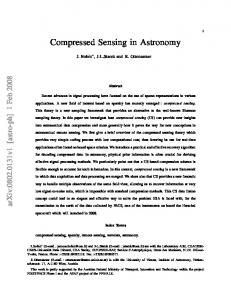
5 VALIDATION IN REAL-WORLD WSN DEPLOYMENT To rigorously validate the proposed CS approach based on WSN routing topology tomography, we deployed our approach in a real‐world outdoor multi‐hop WSN for environmental monitoring [3]. Section 5.1 describes the WSN deployment and our experiment setup. In Sec‐ tion 5.2, we study the sparsification performance of the constructed representation basis. In Section 5.3, we eval‐ uate the data recovery performance of our CS approach, in comparison with three existing CS schemes CDG [8], RS‐CS [7] and CDC [13].
, .
5.1 WSN Testbed and Dataset The multi‐hop WSN in‐situ used in our validation has The Laplacian matrix of a weighted graph G is de‐ been deployed in Pennsylvania [3], for the need of fined as ground‐based data measurements for calibrating and . validating scientific models in hydrology research [24]. Let the weight of all the edges be equal to 1, then the When our CS approach was deployed and validated on of the complement graph is adjacency matrix this WSN testbed, near 80 heterogeneous WSN nodes , 1 if , ∈ (including MICAz, IRIS, and TelosB) had been equipped , and deployed forming a multi‐hop network. The only 0 otherwise. ∑ And , , . We have the Laplacian energy source available for each node is provided by
arXiv:1709.00604 [cs.NI] 2 Sep 2017
7
TABLE 1 THE STATISTICS OF PER-PACKET ROUTING PATH RECOVERY BY RTR SCHEME IN THE WSN TESTBED
Total cycles Average path recovery ratio Best cycle recovery Worst cycle recovery
87 98.38% 100% 93.20%
three NiMH AA rechargeable batteries with a nominal capacity of 2700mAh. The WSN deployment is shown in Figure 4. In terms of hardware of the WSN testbed, MicaZ [25] and IRIS motes [26], each one equipped with an MDA300 data acquisition board [27]. The MDA300 pro‐ vides embedded temperature and humidity sensors. Mi‐ caZ and IRIS have 4K bytes and 8K bytes memory, re‐ spectively. TelosB motes with embedded temperature and humidity sensors. Both TelosB motes and MDA300 acquisition board have ADCs for external sensors, e.g. EC5 (soil moisture sensor) [28]. The base station (sink node), is an IRIS mote with a per‐ manent power supply connected to a computer oper‐ ated as the WSN gateway [29] where the WSN gateway forwards the sensed data stream to the WSN data man‐ agement system over the Internet [30]. Our validation experiments were developed in Ti‐ nyOS 2.1.2 [33]. The deployed routing protocol at the WSN testbed was an extended Collection Tree Protocol (CTP) [34], which introduces a random component into the process of packet forwarding to achieve a better traf‐ fic and energy balance. In our CS validation, we have adopted and deployed the Routing Topology Recovery (RTR) scheme proposed by Liu et al. [18]. In each data collection cycle from M packets received at the sink, the RTR scheme reconstructs each per‐packet routing path. In the RTR implementation, four bytes were used for carrying path measurement independent of the actual hop counts of the routing path, piggy back to each data packet routed towards the sink. Data collected in one acquisition cycle of the WSN testbed, where each WSN node sampled and sent its sensor readings once, form a dataset. In our CS valida‐ tion, we collected datasets from the outdoor WSN testbed in situ for 87 cycles. Table 1 shows the statistics of per‐packet routing path recovery by RTR in our vali‐ dation experiments conducted on the WSN in situ. The longest routing path of packet had 8 hops. The first 10 collected datasets were used as the train‐ ing datasets for constructing the representation basis in our approach while the remaining 77 datasets were used as the test datasets for data recovery performance. Hu‐ midity data were collected from 75 nodes, while soil moisture data were collected from 48 nodes equipped with external soil moisture sensor EC5. The original sen‐ sor readings of each node were also collected in the same
data packet in each cycle in addition to the compressed sensor data to provide the base for the accuracy analysis of our CS approach. 5.2 Performance of Representation Basis We first evaluate the sparseness of the representation ba‐ sis. As described in Section 3, is the 1 coefficient , where ≪ . By vector in the ‐domain with ‖ ‖ keeping only the largest components in magnitude in , we can get the approximation of , and thus the ap‐ ′ . Comparing with gives the proximation performance of the representation basis . The representation basis in our CS approach is con‐ structed as follows: First, construct the underlying graph of WSN based on Equations (8) and (9) with re‐ covered WSN URTGs from path measurements in given training datasets; second, use our devised GLE algo‐ rithm to obtain an appropriate hierarchy decomposition of the underlying graph; third, apply GDL [20] to the ob‐ tained hierarchy decomposition of the underlying graph to construct graph wavelets with given WSN training datasets, and then construct the sparse representation basis based on the constructed graph wavelets. Figure 5 shows an example of the humidity data collected by 75 nodes and the corresponding transform coefficients for the representation basis obtained by our approach with the 10 humidity training datasets. Similarly, Figure 6 shows an example of the soil moisture data from 48 nodes and the corresponding transform coefficients for the representation basis constructed by our approach with the 10 training datasets of soil moisture. As we can see, only very few coefficients are significant in the transform domain. Next, we select the largest k transform coefficients in magnitude of both humidity and soil moisture data, re‐ spectively, to evaluate the sparsification performance of our representation basis. We further compare the spar‐ sification performance of our CS representation basis with those adopting Haar wavelet transformation and DCT (Discrete Cosine Transformation), the two popular transformations used in existing CS schemes such as CDC [13] and CDG [8]. The approximation error (%), de‐ fined as in (10), is employed to evaluate the performance for different CS approaches. Error
∑
⁄ ∑
⁄
100%.
(10)
Figures 7 and 8 show the average sparsification er‐ rors of the 77 test datasets for humidity and soil mois‐ ture signals, respectively. As we can see, the representa‐ tion basis constructed by our method (GLE+graph wavelets via deep learning by GDL) can always lead to very small approximation error even when only keeping a few largest transform coefficients in magnitude. The performances of the three different bases are improved when k becomes larger, and our representation basis al‐
arXiv:1709.00604 [cs.NI] 2 Sep 2017
8
Fig. 7. The sparsification error of humidity datasets estimated by using only the largest k components in magnitude in s.
Fig. 5. Humidity raw signals (top) and the corresponding transform coefficients for our constructed representation basis using the GLE+GDL algorithm (bottom).
Fig. 8. The sparsification error of soil moisture datasets estimated by using only the largest k components in magnitude in s. Fig. 6. Soil moisture raw signals (top) and the corresponding transform coefficients for our constructed representation basis using the GLE+GDL algorithm (bottom).
, ,…, from the WSN testbed in each cycle, we first recover the routing path of each received packet us‐ ing the RTR scheme [18], from which the measurement matrix is reconstructed for the sensor dataset in this ways significantly outperforms the Haar and DCT trans‐ cycle. Then, two CS solvers SL0 [35] and LP [36] are formations. Our method also has very stable perfor‐ adopted to obtain an approximation ′ of in the trans‐ mance on both humidity and soil moisture datasets. For form domain. Finally, the original signal is recovered by humidity data, when keeping only the largest 3 trans‐ computing ′. The recovery accuracy is evaluated form coefficients in magnitude (out of total 75), the ap‐ here using the approximation error defined in (10). proximation error is less than 3.3%, while for soil mois‐ For the evaluation of our compressed sensing ap‐ ture data, keeping only the largest 2 transform coeffi‐ proach CSR, three existing CS schemes CDG [8], RS‐CS cients in magnitude (out of total 48), the approximation (with Horz‐diff transformation) [7] and CDC [13] are error is always less 1.7%. This indicates that the humid‐ used for the comparison. While CSR, CDC and RS‐CS ity and soil moisture signals can be well sparsely repre‐ approaches interplay with routing, CDG does not, and sented using their respective basis obtained by the pro‐ relies on dense random projections which need to collect posed method. data from all WSN nodes. We first set 12 for both humidity and soil mois‐ 5.3 Signal Recovery Accuracy ture data collection in our CS approach CSR. Figure 9 After collecting measurements
arXiv:1709.00604 [cs.NI] 2 Sep 2017
9
Fig. 11. Humidity dataset reconstruction error when M=12, using LP as the solver.
Fig. 9. An example of the routing path (measurement) topology in a data collection cycle for M=12.
Fig. 12. Soil moisture dataset reconstruction errors when M=12, using SL0 as the solver s.
Fig. 10. Humidity dataset reconstruction error when M=12, using SL0 as the solver.
shows an example of the WSN routing topology for the 12 measurements collected from the WSN testbed in our experiments, which was reconstructed by the RTR scheme [18] running at the sink. As we can see, many nodes were not visited in this cycle, which means their data were not collected in CSR, CDC and RS‐CS ap‐ proaches jointly with routing. Fewer visited nodes gen‐ erally can make it more difficult to recover the entire data field. Figures 10 ~ 13 show the reconstruction error for hu‐ midity and soil moisture signals using four different CS approaches, with two solvers: SL0 and LP. As we can see,
Fig. 13. Soil moisture dataset reconstruction errors when M=12, using LP as the solver.
arXiv:1709.00604 [cs.NI] 2 Sep 2017
10
Fig. 17. Soil moisture dataset reconstruction error with different M, using SL0 as the solver.
Fig. 14. Humidity dataset reconstruction errors with different M, using SL0 as the solver.
our CSR with LP solver can always achieve the data re‐ covery with the error less than 7.7% on humidity da‐ tasets and less than 5.0% on soil moisture datasets for any collection cycle, significantly outperforms CDG, CDC and RS‐CS. Note that both CDC and RS‐CS per‐ form worse than CDG and they are sensitive to different datasets collected in different cycles, because only a sub‐ set of the nodes is visited in each individual collection cycle. Our CSR approach overcomes this problem by constructing a much better representation basis as shown in Section 5.2, therefore CSR always outperforms the other three CS approaches for both humidity and soil moisture data. We also note that CDC are very sen‐ sitive to the solver, it performs much better with LP than SL0. Generally, the solver LP outperforms SL0, but LP takes longer computation time. Figures 14 ~ 17 show the reconstruction errors for hu‐ midity and soil moisture signals using four different CS approaches, with different numbers (M) of collected measurements. As we can see, our CSR has excellent performance even when M is very small, with recon‐ struction errors being an order of magnitude less than those of the other three CS approaches even with much larger M. Generally, the performance will improve when M becomes larger, the only exception is CDG with solver LP on soil moisture data. Figure 18 gives an example of the reconstructed hu‐ midity data field by our CSR when only 12 data packets are collected at the sink, in comparison with the original humidity data field. As we can see, while the original humidity data change drastically from sensor node to node, our CSR is still able to recover the entire data field with high fidelity using only 12 measurements. Figures 19 and 20 show the transmission numbers of CSR and CDG for collecting humidity and soil moisture measurements, respectively, for different numbers of re‐ ceived measurements. As we can see, the CSR leads to
Fig. 15. Humidity dataset reconstruction errors with different M, using LP as the solver.
Fig. 16. Soil moisture dataset reconstruction errors with different M, using SL0 as the solver.
arXiv:1709.00604 [cs.NI] 2 Sep 2017
11
Fig. 18. Original signals vs. the reconstructed signals by CSR.
Fig. 19. Transmission numbers on different approaches on humidity dataset.
Fig. 20. Transmission numbers on different approaches on soil moisture dataset.
the drastic reduction of data packet transmission num‐ bers, by an order of magnitude less than those of CDG. This means the drastic radio communication energy conservation by CSR, the great advantage of any CS ap‐ proach successfully interplaying with routing. While both CDC and RS‐CS have the same transmission num‐ bers as CSR in our experiments, due to the employment of the same routing protocol CTP+EER in the experi‐ ments for CDC and RS‐CS as well, CDC and RS‐CS have significantly larger data packet size than that of CSR. This is because CDC and RS‐CS record the original packet path in the data packet along the route, whereas our CSR uses routing topology tomography for path in‐ formation. Consequently, CSR is not only scalable for large‐size WSNs and big data acquisition, but also more resource efficient than CDC and RS‐CS. In summary, rigorous validation and evaluation of our CSR approach versus three existing CS approaches CDG, CDC and RS‐CS were conducted in a real‐world WSN deployment in situ. The results clearly demon‐ strate that CSR approach significantly outperforms CDG, CDC and RS‐CS by reducing data reconstruction errors by an order of magnitude for the entire WSN data field, while drastically reducing wireless communica‐ tion costs, by an order of magnitude, at the same time. This indicates that our CSR approach is a reliable and practical solution to energy efficient data acquisition in multi‐hop large‐scale WSNs. In our experiments, CSR can successfully recover the entire data field of the real‐ world multi‐hop WSN in situ with very small errors, when only 16% of data packets (i.e., 12 randomly se‐ lected nodes out of total 75 sensor nodes in the WSN testbed) needed to be collected at the sink.
6 CONCLUTION In principle, CS based data acquisition in multi-hop WSN deployments has a great potential to further significantly reduce sensor nodes’ transmissions via the interplaying with the network dynamic routing to facilitate wireless big data acquisition. In practice, however, two critical issues have to be effectively addressed before the potential said above can be realized in any large-scale real-world WSN deployment. The first issue is how to effectively obtain the dynamic routing information for each received packet at the sink, since simply recording path along the route is neither scalable nor resourceefficient. The second issue, originally identified by Quer et al. [7], is how to design a suitable representation basis for realworld signals that has good sparsification and incoherence with the measurement matrix derived from dynamic WSN data packet routing, because it has been found [7] that commonly used transformations including DCT and Haar Wavelet for constructing representation basis, as well as the Horz-diff transformation [7], all suffered from large recovery errors for real WSN data.
arXiv:1709.00604 [cs.NI] 2 Sep 2017
12
In this paper, we attempt to address these critical open questions and present a novel CS approach called CSR for multi-hop WSN data acquisition based on dynamic routing topology tomography. Our CSR approach has two distinguishing characteristics. First, CSR introduces the use of WSN routing topology tomography into CS approach and thus provides a practical and elegant solution for large-scale WSN data acquisition based on effective interplaying with dynamic routing. We show that the adoption of routing matrix as measurement matrix in compressed sensing in recovering k-sparse sensor signals in WSN can achieve feasible estimation with bounded errors. As shown in our real-world WSN experiments, our CSR approach considerably reduces transmission numbers (e.g., 58 transmissions in CSR versus 900 transmissions in CDG, for collecting 12 measurements at the sink), resulting in an order of magnitude less in energy consumption compared to CDG, and also significant reduction of transmission costs compared to CDC and RS-CS, thus extending the lifetime of real-world outdoor WSN deployments. Second, CSR provides a systematic method to construct an optimized representation basis with both good sparsification and incoherence properties for various given classes of signals, and therefore drastically reduces WSN data recovery errors by an order of magnitude compared to existing CS schemes CDG, CDC and RS-CS. Therefore, the proposed approach is expected to significantly improve the state of art of CS based approaches for WSN data acquisition, and to facilitate the CS application in large-scale multi-hop outdoor WSN systems for various data gathering. Our approach is deployed for a real-world outdoor WSN testbed and is rigorously validated and evaluated via the WSN deployment in situ operated under highly dynamic communication environment for environmental monitoring. To the best of our knowledge, our work represents the first demonstration and performance analysis of CS approaches applied to realworld WSN deployment in situ jointly with routing for data acquisition with actual routing protocol in operation. Our approach via deep learning seems very effective, as only 10 training datasets were used in constructing the representation basis in our experiments. It is expected that the presented systematic method in our CSR approach for constructing an optimized representation basis can be in general adopted to any other CS schemes to significantly improve their data recovery fidelity in big data acquisition.
REFERENCES [1]
X. Mao, X. Miao, Y. He, X.Y. Li, and Y. Liu. "CitySee: Urban CO 2 monitoring with sensors." In INFOCOM, 2012 Proceedings IEEE, pp. 1611-1619. IEEE, 2012.
[2]
Y. Liu, Y. He, M. Li, J. Wang, K. Liu, and X. Li. "Does wireless sensor network scale? A measurement study on GreenOrbs." IEEE Transactions on Parallel and Distributed Systems 24, no. 10 (2013): 1983-1993.
[3]
M. Navarro, T. W. Davis, G. Villalba, Y. Li, X. Zhong, N. Erratt, X. Liang, and Y. Liang. "Towards long-term multi-hop WSN deployments for environmental monitoring: An experimental network evaluation." Journal of Sensor and Actuator Networks 3, no. 4 (2014): 297-330.
[4]
M.Z.A. Bhuiyan, G. Wang, J. Cao, and J. Wu. "Sensor placement with multiple objectives for structural health monitoring." ACM Transactions on Sensor Networks (TOSN) 10, no. 4 (2014): 68.
[5]
E.J. Candès, J. Romberg, and T. Tao. "Robust uncertainty principles: Exact signal reconstruction from highly incomplete frequency information." IEEE Transactions on information theory 52, no. 2 (2006): 489-509.
[6]
D.L. Donoho. "Compressed sensing." IEEE Transactions on information theory 52, no. 4 (2006): 1289-1306.
[7]
G. Quer, R. Masiero, D. Munaretto, M. Rossi, J. Widmer, and M. Zorzi. "On the interplay between routing and signal representation for compressive sensing in wireless sensor networks." In Information Theory and Applications Workshop, 2009, pp. 206-215. IEEE, 2009.
[8]
C. Luo, F. Wu, J. Sun, and C. W. Chen. "Compressive data gathering for large-scale wireless sensor networks." In Proceedings of the 15th annual international conference on Mobile computing and networking, pp. 145-156. ACM, 2009.
[9]
L. Xiang, J. Luo, and A. Vasilakos. "Compressed data aggregation for energy efficient wireless sensor networks." In Sensor, mesh and ad hoc communications and networks (SECON), 2011 8th annual IEEE communications society conference on, pp. 46-54. IEEE, 2011.
[10] L. Xiang, J. Luo, and C. Rosenberg. "Compressed data aggregation: Energy-efficient and high-fidelity data collection." IEEE/ACM Transactions on Networking (TON) 21, no. 6 (2013): 1722-1735. [11] L. Kong, M. Xia, X.Y. Liu, M.Y. Wu, and X. Liu. "Data loss and reconstruction in sensor networks." In INFOCOM, 2013 Proceedings IEEE, pp. 1654-1662. IEEE, 2013. [12] X. Wu, and M. Liu. "In-situ soil moisture sensing: measurement scheduling and estimation using compressive sensing." In Proceedings of the 11th international conference on Information Processing in Sensor Networks, pp. 1-12. ACM, 2012. [13] X.Y. Liu, Y. Zhu, L. Kong, C. Liu, Y. Gu, A. V. Vasilakos, and M.Y. Wu. "CDC: Compressive data collection for wireless sensor networks." IEEE Transactions on Parallel and Distributed Systems 26, no. 8 (2015): 2188-2197. [14] H. Zheng, F. Yang, X. Tian, X. Gan, X. Wang, and S. Xiao. "Data gathering with compressive sensing in wireless sensor networks: a random walk based approach." IEEE Transactions on Parallel and Distributed Systems 26, no. 1 (2015): 35-44. [15] X. Lu, D. Dong, X. Liao, and S. Li. "PathZip: Packet path tracing in wireless sensor networks." In Mobile Adhoc and Sensor Systems (MASS), 2012 IEEE 9th International Conference on, pp. 380-388. IEEE, 2012.
ACKNOWLEDGMENT The authors wish to thank X. Zhong at IUPUI, and G. Vil‐ lalba, F. Plaza, T. A. Slater and Dr. X. Liang at the University of Pittsburgh for their great help and support in the WSN testbed deployment of the CSR approach. This work was supported in part by the U.S. National Science Foundation under CNS‐1320132.
[16] Y. Gao, W. Dong, C. Chen, J. Bu, G. Guan, X. Zhang, and X. Liu. "Pathfinder: Robust path reconstruction in large scale sensor networks with lossy links." In Network Protocols (ICNP), 2013 21st IEEE International Conference on, pp. 1-10. IEEE, 2013. [17] Z. Liu, Z. Li, M. Li, W. Xing, and D. Lu. "Path reconstruction in dynamic wireless sensor networks using compressive sensing." In Proceedings of the 15th ACM international symposium on Mobile ad hoc networking and computing, pp. 297-306. ACM, 2014.
arXiv:1709.00604 [cs.NI] 2 Sep 2017
13
[18] R. Liu, Y. Liang, and X. Zhong. "Monitoring Routing Topology in Dynamic Wireless Sensor Network Systems." In Network Protocols (ICNP), 2015 IEEE 23rd International Conference on, pp. 406-416. IEEE, 2015. [19] Yi. Gao, W. Dong, C. Chen, J. Bu, W. Wu, and X. Liu. "iPath: Path inference in wireless sensor networks." IEEE/ACM Transactions on Networking (TON) 24, no. 1 (2016): 517-528. [20] R. Rustamov, and L. J. Guibas. "Wavelets on graphs via deep learning." In Advances in neural information processing systems, pp. 998-1006. 2013. [21] S. G. Mallat. "A theory for multiresolution signal decomposition: the wavelet representation." IEEE transactions on pattern analysis and machine intelligence 11, no. 7 (1989): 674-693. [22] R. Hamon, P. Borgnat, P. Flandrin, and C. Robardet. "Discovering the structure of complex networks by minimizing cyclic bandwidth sum." arXiv preprint arXiv:1410.6108 (2014). [23] M. H. Firooz, and S. Roy. "Link delay estimation via expander graphs." IEEE Transactions on Communications 62, no. 1 (2014): 170-181. [24] G. Villalba, F. Plaza, X. Zhong, T. W. Davis, M. Navarro, Y. Li, T. A. Slater, Y. Liang, and X. Liang. "A Networked Sensor System for the Analysis of Plot-Scale Hydrology." Sensors 17, no. 3 (2017): 636. [25] Micaz wireless measurement system. 2016. http://www.memsic.com/wireless-sensor-networks/.
Available
at
[26] Iris wireless measurement system. 2016. http://www.memsic.com/wireless-sensor-networks/.
Available
at
[27] MDA300 data acquisition board. 2016. http://www.memsic.com/wireless-sensor-networks/.
Available
at
[28] Ec-5 small soil moisture sensor. 2016. Available at https://www.decagon.com/en/soils/volumetric-water-content-sensors/ec-5-lowest-costvwc/. [29] N. Erratt, and Y. Liang. "The design and implementation of a general WSN gateway for data collection." Wireless Communications and Networking Conference (WCNC), 2013 IEEE. IEEE, 2013. [30] M. Navarro, D. Bhatnagar, and Y. Liang. "An integrated network and data management system for heterogeneous WSNs." In Mobile Adhoc and Sensor Systems (MASS), 2011 IEEE 8th International Conference on, pp. 819-824. IEEE, 2011. [31] J. Haupt, W. U. Bajwa, M. Rabbat, and R. Nowak. "Compressed sensing for networked data." IEEE Signal Processing Magazine 25, no. 2 (2008): 92-101. [32] W. Wang, M. Garofalakis, and K. Ramchandran. "Distributed sparse random projections for refinable approximation." In Proceedings of the 6th international conference on Information processing in sensor networks, pp. 331-339. ACM, 2007. [33] TinyOS. 2016 Available at http://webs.cs.berkeley.edu/tos/ [34] M. Navarro, and Y. Liang. "Efficient and Balanced Routing in EnergyConstrained Wireless Sensor Networks for Data Collection." In EWSN, pp. 101-113. 2016. [35] H. Mohimani, M. Babaie-Zadeh, and C. Jutten. "A Fast Approach for Overcomplete Sparse Decomposition Based on Smoothed l0 Norm." IEEE Transactions on Signal Processing 57, no. 1 (2009): 289-301. [36] Sparse lab. 2016. Available at http://sparselab.stanford.edu/