Applied Mathematics & Information Sciences – An International Journal
5(1) (2010), 20-33
Applications of the Variational Monte Carlo Method to the Two-Electron Atom S. B. Doma1 and F. N. El-Gammal2 1
Faculty of Information Technology and Computer Sciences, Sinai University, El-Arish, North Sinai, Egypt. 2
Mathematics Department, Faculty of Science, Menofia University, Shebin El-Kom, Egypt. Email Address:
[email protected], Received June 22, 2009; Revised March 21, 2010; Accepted May 02, 2010
The Variational Monte Carlo method is used to evaluate the ground state as well as the lowest four excited states of the helium atom. Trial wave functions depending on variational parameters are presented. The energies are plotted versus the variational parameters. The obtained results are of good agreement with the exact data. Pervious results are presented for comparison. Keywords: Variational Monte Carlo method, Excited states, Helium atom.
1
Introduction
Quantum Monte Carlo (QMC) methods have become a powerful tool in Quantum Mechanics calculations [1]. Quantum Monte Carlo (QMC) techniques provide a practical method for solving the many-body Schr¨odinger equation. It is commonly used in physics to simulate complex systems that are of random nature in statistical physics. There are many versions of the QMC methods that are used to solve the Schr¨odinger equation for the ground state energy of a quantum particle including the diffusion Monte Carlo method [2], which is used to solve the time-dependent Schr¨odinger equation. Another method is the Green’s function Monte Carlo which has been extended to multiple states with the same quantum numbers [3]. The simplest of (QMC) methods is the VMC technique which has become a valuable tool of the quantum chemist calculations [4-6]. It is based on evaluating a high-dimensional integral by sampling the integrand using a set of randomly generated points. It can be shown that the integral converges faster by using VMC technique rather than more conventional techniques based on sampling the integrand on a regular grid for problems involving more than few dimensions. Moreover, the statistical error in the estimate of the integral decreases as the square root of the number of points sampled,
21
Variational Monte Carlo Method to the Two-Electron Atom
irrespective of the dimensionality of the problem. The major advantage of this method is the possibility to freely choose the analytical form of the trial wave function which may contain highly sophisticated term in such a way that electron correlation is explicitly taken into account. This is an important feature valid for QMC methods, which are therefore extremely useful to study physical cases where the electron correlation plays a crucial role.
2
Variational Monte Carlo Calculations
The VMC method [7] is based on a combination of two ideas namely the variational principal and Monte Carlo evaluation of integrals using importance sampling based on the Metropolis algorithm. It is used to compute quantum expectation values of an operator. In particular, if the operator is the Hamiltonian, its expectation value is the varitional energy EV M C
R ∗ ˆ T (R)dR Ψ (R)HΨ = R T∗ ΨT (R)ΨT (R)dR
(2.1)
where ΨT is a trial wave function and R is the 3N-dimensional vector of the electron coordinates. According to the Varitional principal, the expectation value of the Hamiltonian is an upper bound to the exact ground state energy E0 that is, EV M C ≥ E0 . To evaluate the integral in Eq. (2.1) we construct first a trial wave function Ψα T (R) depending on α variational parameters α = (α1 , α2 , .........αN ) and then vary the parameters to obtain minimum energy. Variational Monte Carlo calculations determine EV M C by writing it as Z EV M C = P (R)EL (R)d(R) Where P (R) = R
|ΨT (R)|2 |ΨT (R)|2 dR ˆ
T is positive everywhere and interpreted as a probability distribution and EL = HΨ ΨT is the local energy function. The value of EL is evaluated using a series of points Rij proportional to P (R). At each of these points the weighted average, R 2 Ψ (R)EL dR hEL i = R T 2 ΨT (R)dR
is evaluated. After a sufficient number of evaluations the VMC estimate of EV M C will be:
EV M C
N M 1 1 XX = hEL i = lim lim EL (Rij) N −→∞ M →∞ N M i=1 J=1
(2.2)
22
S. B. Doma et al.
where M is the ensemble size of random numbers {R1 , R2 , .........RN } and N is the number of ensembles. These ensembles so generated must reflect the distribution function itself. A given ensemble is chosen according to the Metropolis algorithm [8]. This method uses an acceptance and rejection process of random numbers that have a frequency probability distribution like Ψ2 . The acceptance and rejection method is performed by obtaining a random number from the probability distribution, P (R) then testing its value to determine if it will be acceptable for use in approximation of the local energy. Random numbers may be generated using a variety of methods [9]. After an ensemble of random numbers is generated, the acceptance and rejection criterion is such that the probability of moving from an initial random number of the ensemble Ri to a new random number Rk is defined according to the ratio A=
Ψ2 (Rk ) Ψ2 (Ri )
If A is larger than one, this trial step is accepted (i.e. we put Ri+1 = Rk )and the new Rk is a member of the next ensemble. While if A is less than one, the step is accepted with probability A. This latter is conveniently accomplished by comparing A with random number η uniformly distributed in the interval [0,1] and accepting the step if η < A. If the trial step is not accepted, then it is rejected, and we put Ri+1 = Ri . This process is repeated for each member of an ensemble and is done in order to broaden subsequent ensembles for a wider sampling range. Any arbitrary point R0 can be used as the starting point for the random walk. The accepted ensembles will be used to evaluate the Variational Monte Carlo estimate for the average energy according to Eq. (2.2). In our work the broadening of the ensemble is achieved according to Y = R(K) + DELT A ∗ (RAN D0(SEED) − 0.5) Where, Y is the new value Rk to be tested and R(K) is the value Ri of the previously accepted ensemble for K = i. The function RAN D returns a uniform random number between 0 and 1, and is a nonintrinsic function. The range width is determined by DELT A, adjusted to suit particular needs, and the value 0.5 ensures the availability of negative numbers. The random number generator only produces numbers between 0 and 1, so there will be an initial maximum random value and an initial minimum random value. These maximum and minimum values in the new accepted ensemble, {R(K)}, are kept as subsequent ensemble grow in range. Finally, it is important to calculate the standard deviation of the energy, s σ=
hEL2 i − hEL i2 M (N − 1)
(2.3)
Variational Monte Carlo Method to the Two-Electron Atom
3
23
The Trial Wave Function
The choice of trial wave function is critical in VMC calculations. How to choose it is however a highly non-trivial task. All observables are evaluated with respect to the probability distribution P (R) = R
|ΨT (R)|2 |ΨT (R)|2 dR
generated by the trial wave function. The trial wave function must approximate an exact eigen state in order that accurate results are to be obtained. A good trial wave function should exhibit much of the same features as does the exact wave function. One possible guideline in choosing the trial wave function is the use of the constraints about the behavior of the wave function when the distance between one electron and the nucleus or two electrons approaches zero. These constraints are called ”cusp conditions” and are related to the derivative of the wave function. Usually the correlated wave function,Ψ, that is used in the VMC calculations is built as the product of a symmetric correlation factor, f , which includes the dynamic correlation among the electrons, times a model wave function, ϕ, that provides the correct properties of the exact wave function such as the spin and the angular momentum of the atom, and is antisymmetric in the electronic coordinates Ψ = f ϕ. With this type of wave function, and by using different correlation factor, the ground-states of atoms from He to Kr have been extensively studied [10-12]. The aim of the present paper is to extend this methodology to obtain the ground and the excited states of the helium atom. This will be done within the context of the accurate Born-Oppenheimer approximation, which is based on the notion that the heavy nucleus is moving slowly compared to the much lighter electrons.
4
The Statement of the Problem
For a nucleus with charge Z and infinite mass the non-relativistic Hamiltonian for the two-electron atom, in atomic units (a. u), reads [13]: H=
1 2 2 Z Z 1 (p +p )− − + 2 1 2 r1 r2 r12
(4.1)
where r1 and r2 denote the relative coordinate distances of the two electrons with respect to the nucleus and r12 is the distance between the two electrons i.e r12 = |r1 − r2 |. In Hylleraas coordinates the above Hamiltonian can be written as [14]: 1 ∂2 2 ∂ ∂2 2 ∂ ∂2 H=− ( 2 + + + + 2ˆr1 · ˆr12 ) 2 2 ∂r1 r1 ∂r1 ∂r12 r12 ∂r12 ∂r1 ∂r12 1 ∂2 2 ∂ ∂2 2 ∂ ∂2 Z Z 1 − ( 2 + + + − 2ˆr2 · ˆr12 )− − + 2 2 ∂r2 r2 ∂r2 ∂r12 r12 ∂r12 ∂r2 ∂r12 r1 r2 r12
24
S. B. Doma et al.
where ˆr1 ,ˆr2 and ˆr12 denote the unit vectors of the corresponding distances. In writing Eq. (4.1) we have taken into account the Coulomb interactions between the particles, but have neglected small corrections arising from spin-orbit and spin-spin interactions. The electronic eigenvalue is determined by the Schr¨odinger equation: HΨ(r1 , r2 ) = EΨ(r1 , r2 )
(4.2)
where Ψ(r1 , r2 ) is the electronic wave function. Our goal is, then, to solve the six-dimensional partial differential eigenvalue equation, Eq. (4.2), for the lowest eigenvalue.
5
The Ground State of the Helium Atom For the ground state of the helium atom the trial wave function used in this paper is given by [15]: Ψ(r1 , r2 ) = ϕ(r1 )ϕ(r2 )f (r12 )
(5.1)
where ϕ(ri ) is the single-particle wave function for particle i, and f (r12 ) account for more complicated two-body correlations. For the helium atom, we have placed both electrons in the lowest hydrogenic orbit 1s to
Figure 5.1: The Ground state energy versus the variational parameter β. calculate the ground state. A simple choice for ϕ(ri ) is ϕ(ri ) = exp(−ri /a)
(5.2)
with the variational parameter a to be determined. The final factor in the trial wave function, f ,expresses the correlation between the two electrons due to their Coulomb repulsion. That is, we expect f to be small when r12 is small and to approach a large constant value as the electrons become well separated. A convenient and reasonable choice for f is r ] (5.3) f (r) = exp[ α(1 + βr) where α and β are additional positive variational parameters. The variational parameter β controls the distance over which the trial wave function heals to its uncorrelated value as the two electrons separate. Using the cusp conditions [16] we can easy verify that the variational parameters a, α satisfy the equations: 1 , α=2 (5.4) 2 Thus β is the only variational parameter at our disposal. With the trial wave function specified by Eq. (5.1), explicit expression can be worked out for the local energy EL (R) in terms of the values and derivatives of ϕ and f. a=
Variational Monte Carlo Method to the Two-Electron Atom
25
Figure 5.2: a,b The energies for 23 S and 23 S states respectively, versus the variational parameter β.
Figure 5.3: a,b The energies for 21 P and 23 P states respectively, versus the variational parameter β.
26
S. B. Doma et al.
6
Excited States of the Helium Atom
In this section we present the trial function used in our calculations for excited states [13]. For the lowest ortho (space-antisymmetric) state 23 S, a trial wave function which is antisymmmetrized product of an inner (1s) orbital u1s corresponding to effective charge Zi and an outer (2s) orbital v2s corresponding to effective charge Z0 can be written in the form: Ψ23 S (r1 , r2 ) = N [u1s (r1 )v2s (r2 ) − v2s (r1 )u1s (r2 )]f (r12 )
(6.1)
where, u1s (r) = exp(−Zi r) v2s (r) = (1 − Z0 r/2) exp(−Z0 r/2) and N is a normalization constant. For the 21 S state which is para (space-symmetric), we construct a simple wave function which would be space-symmeric as Ψ21 S (r1 , r2 ) = N [u1s (r1 )v2s (r2 ) + v2s (r1 )u1s (r2 )]f (r12 )
(6.2)
u1s (r) = exp(−2r) v2s (r) = exp(−τ1 r) − Cr exp(−τ2 r) where τ1 , τ2 and C are variational parameters. The trial wave function for 21 P and 23 P states are given by Ψ21 P (r1 , r2 ) = N [u1s (r1 )v2pm (r2 ) + v2pm (r1 )u1s (r2 )]f (r12 )
(6.3)
Ψ23 P (r1 , r2 ) = N [u1s (r1 )v2pm (r2 ) − v2pm (r1 )u1s (r2 )]f (r12 )
(6.4)
With u1s (r) and v2pm (r1 ) take the form u1s (r) = exp(−Zi r) v2pm (r) = r exp(−Z0 r/2)Y1,m (θ, φ),
m = 0, ±1
(6.5)
where, Zi , Z0 are variational parameters and θ, φ denoting the angular variables for each electron.
Energies for the ground state and first four excited states together with the standard deviation σ, the exact data and pervious results for comparison. EV M C σ Exact Data [13] Pervious Results [17] Ground state -2.903731 0.0034 -2.9037 -2.90372 23 S State -2.175005 0.0013 -2.17522 -2.175 1 1 2 S State -2.145965 0.0004 -2.146 -2.14597 1 2 P State -2.123835 0.0002 -2.124 -2.12384 23 P State -2.133116 0.0004 -2.133 -2.13316
7
Results and Conclusions
The Monte Carlo process described here has been employed for the ground and lowest four excited states of helium atom. All energies obtained in atomic units i.e (~ = e = me = 1). All the values of the variational
Variational Monte Carlo Method to the Two-Electron Atom
27
parameter (rather than β) appear in the trial wave functions of the excited states are already optimized in [13]. Fig.5.1 shows the ground state energy versus the variational parameter β. For the 23 S state, the energy is obtained by taking the vaiational parameters Zi , Z0 as Zi = 2.01 and Zi = 1.53. Fig.5. 2-a shows the energy of the state 23 S versus the variational parameter β. The variational parameters appear in the trial wave function for the 21 S state are taken as: τ1 = 0.865, τ2 = 0.522 and C = 0.432784. Fig.5 .2-b shows the energy for 21 S state versus the variational parameter β. q
3 In our work we take Y1,m (θ, φ) in Eq. (6.5) to be Y1,0 (θ, φ) = cos θ. For the 21 P state the energy 4π is obtained by taking the vaiational parameters Zi , Z0 as: Zi = 2 and Z0 = .97. Fig.5. 3-a shows the energy for the state 21 P versus the variational parameter β. The variational parameters Zi and Z0 appearing in the trial wave function for the 23 P state are taken to be Zi = 1.99 and Z0 = 1.09. Fig.5. 3-b shows the energy for the state 23 P versus the variational parameter β. In Table-1 we present the resulting values of the energies and the crossponding standard deviation σ. The exact data [13] and pervious results [17] are introduced for comparison. It is clear that the obtained results are in good agreement with corresponding exact and previous results.
References [1] N. Umezawa, S. Tsuneyuki,Excited electronic state calculations by the transcorrelated variational Monte Carlo method: Application to a helium atom,J. Chem. Phys.121.2004. [2] Shao, Y. Tang, Diffusion Monte Carlo analysis of thecrossover from three to two dimensions for trapped Bose gases, J. Physc. B. 404.(2009), 217-222. [3] S. C. Pieper, Nucl. Quantum Monte Carlo Calculations of Light Nuclei, Phys. A. 751, (2005), 516c-532c. [4] E. Buend´ıa, F. J. G´alvez, A. Sarsa, Explicitly correlated energies for neutral atoms and cations with 37 ≤ Z ≤ 54, Chem. Phys. Lett. 465 (2008), 190-192. [5] S. A. Alexander, R. L. Coldwell, Oscillator strengths of helium computed using Monte Carlo methods, J Chem Phys.124 (2006), 054104. [6] T. Watanabe, H. Yokoyama, Y. Tanaka, J. Inoue, M. Ogata, Variational Monte Carlo studies of a tJ model on an anisotropic triangular lattice, Physc. C. 426-431 (2005), 289-294. [7] S. Pottorf, A. Puzer, M. Y. Chou, J. E. Husbun, The simple harmonic oscillator ground state using a variational Monte Carlo method, Eur. J. Phys. 20 (1999), 205-212. [8] N. Metropolis, A. W. Rosenbluth, N. M. Rosenbluth, A. M. Teller, E. Teller, Equations of state calculations by fast computing machines,J. Chem. Phys.21 (1953), 1087-92. [9] R. W. Hamming, Numerical Methods for Scientists and Engineers, 2nd edn New York: McGraw-Hill, 1973. [10] F. J. G´alvez, E. Buend´ıa, A. Sarsa , Atomic properties from energy-optimized wave functions,J. Chem. Phys. 115, (2001),1166. [11] N. Umezawa, S. Tsuneyuki, T. Ohno , K. Shiraishi, T. Chikyow, A Practical Treatment for the Three-body Interactions in the Transcorrelated Variational Monte Carlo Method: Application to Atoms from Lithium to Neon, J. Chem. Phys.122 (2005), 224101. [12] E. Buend´ıa, F.J. G´alvez, A. Sarsa, Correlated wave functions for the ground state of the atoms Li through Kr, Chem. Phys. Lett.428 (2006), 241-244. [13] B. H. Bransden, C. J. Joachain, Physics of Atoms and Molecules, Longman Scientific and Technical, London, 2003. [14] M. B. Ruiz, Hylleraas Method for Many-Electron Atoms. I. The Hamiltonian, Int. J. Quantum Chem.101 (2005), 246-260.
28
S. B. Doma et al.
[15] S. E. Koonin, Computional Physics, Addison-Wesley Publishing Company Inc San Juan. Wokingham, United Kingdom, 1986. [16] T. A. Galek, N. C. Handy, A. J. Cohen, G. K . Chan, HartreeFock orbitals which obey the nuclear cusp condition, Chem. Phys. Lett.404 (2005), 156-163. [17] S. A. Alexander, R. L. Coldwell, Electric Quadrupole Oscillator Strengths of Helium, Int. J. Quantum Chem.108 (2008), 2813-2818. Fatma El Zahraa NaguibB, Sc. of Mathematics, Faculty of Science, Menoufia University, Shebin El-Kom, Egypt (1998). M. Sc. of Applied Mathematics, Faculty of Science, Menoufia University, Shebin El-Kom, Egypt (2006). Demonstrator of Mathematics at Department of Mathematics, Faculty of Science, Menoufia University, Shebin El-Kom, Egypt from 2001 to 2006. Assistance Lecturer of Applied Mathematics at the Department of Mathematics, Faculty of Science, Menoufia University, Shebin El-Kom, Egypt since 2006.