Floyd, Iron Maiden, Slipknot, Riverside, Led Zeppelin, Tool, Linkin Park, and many others, and the Chronix Aggression online radio station. They are all ...
Applications on emerging paradigms in parallel computing by Abhinav Sarje
A dissertation submitted to the graduate faculty in partial fulfillment of the requirements for the degree of DOCTOR OF PHILOSOPHY
Major: Computer Engineering Program of Study Committee: Srinivas Aluru, Major Professor Baskar Ganapathysubramanian Phillip H. Jones Patrick S. Schnable Joseph Zambreno
Iowa State University Ames, Iowa 2010 c Abhinav Sarje, 2010. All rights reserved. Copyright
ii
TABLE OF CONTENTS
LIST OF FIGURES . . . . . . . . . . . . . . . . . . . . . . . . . . . . . . . . . .
iv
LIST OF TABLES . . . . . . . . . . . . . . . . . . . . . . . . . . . . . . . . . . .
x
ABSTRACT . . . . . . . . . . . . . . . . . . . . . . . . . . . . . . . . . . . . . . .
xiii
CHAPTER 1. INTRODUCTION . . . . . . . . . . . . . . . . . . . . . . . . .
1
1.1
Emerging Paradigms in Parallel Computing . . . . . . . . . . . . . . . . . . . .
1
1.2
Emerging Architectures . . . . . . . . . . . . . . . . . . . . . . . . . . . . . . .
2
1.2.1
The Cell Processor . . . . . . . . . . . . . . . . . . . . . . . . . . . . . .
2
1.2.2
Graphics Processors . . . . . . . . . . . . . . . . . . . . . . . . . . . . .
4
1.2.3
Algorithms and Applications on Emerging Architectures . . . . . . . . .
7
1.2.4
Contributions on the Emerging Architectures Paradigm . . . . . . . . .
8
Parallel Processing with Cloud Computing . . . . . . . . . . . . . . . . . . . . .
9
1.3
1.3.1
MapReduce Paradigm . . . . . . . . . . . . . . . . . . . . . . . . . . . .
10
1.3.2
Applications on MapReduce . . . . . . . . . . . . . . . . . . . . . . . . .
11
1.3.3
Contributions on the Cloud Computing Paradigm . . . . . . . . . . . .
11
CHAPTER 2. GENOMIC ALIGNMENTS ON HETEROGENEOUS MULTICORE PROCESSORS
. . . . . . . . . . . . . . . . . . . . . . . . . . . . . .
13
2.1
Genomic Alignments . . . . . . . . . . . . . . . . . . . . . . . . . . . . . . . . .
13
2.2
Global/Local Alignment . . . . . . . . . . . . . . . . . . . . . . . . . . . . . . .
15
2.2.1
Reducing Memory Usage . . . . . . . . . . . . . . . . . . . . . . . . . .
16
2.2.2
Space-Efficient Global Alignment on CBE . . . . . . . . . . . . . . . . .
17
2.2.3
Analyzing Communication Complexity on the Cell BE . . . . . . . . . .
20
2.2.4
Optimizing for efficient usage of SPE hardware and memory . . . . . . .
23
2.2.5
Performance Results and Discussions . . . . . . . . . . . . . . . . . . . .
25
Spliced Alignment on CBE . . . . . . . . . . . . . . . . . . . . . . . . . . . . .
27
2.3.1
Performance Results and Discussions . . . . . . . . . . . . . . . . . . . .
28
Syntenic Alignment on CBE . . . . . . . . . . . . . . . . . . . . . . . . . . . . .
29
2.4.1
Performance Results and Discussions . . . . . . . . . . . . . . . . . . . .
30
Ending Notes . . . . . . . . . . . . . . . . . . . . . . . . . . . . . . . . . . . . .
32
2.3 2.4 2.5
iii CHAPTER 3. PAIRWISE COMPUTATIONS ON MULTI- AND MANYCORE PROCESSORS 3.1 3.2
3.3
3.4
3.5
3.7
34
Pairwise Computations . . . . . . . . . . . . . . . . . . . . . . . . . . . . . . . .
34
3.1.1
Problem Definition: Generalized Pairwise Computations . . . . . . . . .
36
Scheduling Pairwise Computations on Cell Processors . . . . . . . . . . . . . .
37
3.2.1
The Basic Scheduling Scheme . . . . . . . . . . . . . . . . . . . . . . . .
37
3.2.2
Tiling . . . . . . . . . . . . . . . . . . . . . . . . . . . . . . . . . . . . .
38
3.2.3
Determining Tile Size . . . . . . . . . . . . . . . . . . . . . . . . . . . .
39
3.2.4
Extending to Higher Dimensions . . . . . . . . . . . . . . . . . . . . . .
42
3.2.5
Parallelizing Across Multiple Cell Processors . . . . . . . . . . . . . . .
44
Applications with Pairwise Computations on Cell Processors . . . . . . . . . .
45
3.3.1
Lp -norm Computations . . . . . . . . . . . . . . . . . . . . . . . . . . .
45
3.3.2
Lp -norm Performance Results . . . . . . . . . . . . . . . . . . . . . . . .
47
3.3.3
Mutual Information Computations . . . . . . . . . . . . . . . . . . . . .
49
3.3.4
MI Performance Results . . . . . . . . . . . . . . . . . . . . . . . . . . .
50
Pairwise Computations on Graphics Processors . . . . . . . . . . . . . . . . . .
53
3.4.1
Efficient All-pairs Computations on a GPU . . . . . . . . . . . . . . . .
54
3.4.2
Generalizing to Higher Dimensions . . . . . . . . . . . . . . . . . . . . .
55
Analyzing the Performance on GPU . . . . . . . . . . . . . . . . . . . . . . . .
56
3.5.1
Features and Constraints . . . . . . . . . . . . . . . . . . . . . . . . . .
57
3.5.2
Varying Thread Block / Subtile size r × c . . . . . . . . . . . . . . . . .
58
Number of Subtiles s in a Tile . . . . . . . . . . . . . . . . . . . . . . .
60
3.5.4
Input Vectors Slice Size ds . . . . . . . . . . . . . . . . . . . . . . . . . .
62
3.5.5
Choosing the Parameter Values . . . . . . . . . . . . . . . . . . . . . . .
62
Performance of Pairwise Computations on Various Processors . . . . . . . . . .
63
3.6.1
Single Precision Performance Results . . . . . . . . . . . . . . . . . . . .
64
3.6.2
Double Precision Performance Results . . . . . . . . . . . . . . . . . . .
65
End Notes . . . . . . . . . . . . . . . . . . . . . . . . . . . . . . . . . . . . . . .
67
3.5.3
3.6
. . . . . . . . . . . . . . . . . . . . . . . . . . . . . .
CHAPTER 4. AN ABSTRACT FRAMEWORK FOR TREES ON CLOUDS 68 4.1
The Proposed Framework . . . . . . . . . . . . . . . . . . . . . . . . . . . . . .
68
4.1.1
Tree Compute . . . . . . . . . . . . . . . . . . . . . . . . . . . . . . . .
69
Casting Tree Operations into the Framework . . . . . . . . . . . . . . . . . . .
70
4.2.1
Local Computations . . . . . . . . . . . . . . . . . . . . . . . . . . . . .
70
4.2.2
Upward Tree Accumulation . . . . . . . . . . . . . . . . . . . . . . . . .
71
4.2.3
Downward Tree Accumulation . . . . . . . . . . . . . . . . . . . . . . .
71
4.2.4
Nodes within a Distance Range . . . . . . . . . . . . . . . . . . . . . . .
71
4.3
Algorithms for Building the Framework . . . . . . . . . . . . . . . . . . . . . .
72
4.4
Implementation of the Framework . . . . . . . . . . . . . . . . . . . . . . . . .
74
4.2
iv
4.5
4.6
4.4.1
Generic Programming, Concept and Model . . . . . . . . . . . . . . . .
74
4.4.2
Concept Definitions for the Framework . . . . . . . . . . . . . . . . . . .
75
4.4.3
Implementation Details . . . . . . . . . . . . . . . . . . . . . . . . . . .
77
Sample Applications and Performance . . . . . . . . . . . . . . . . . . . . . . .
78
4.5.1
Finding All k-Nearest Neighbors (k-NN) . . . . . . . . . . . . . . . . . .
78
4.5.2
Performance Results of k-NN Implementation . . . . . . . . . . . . . . .
80
4.5.3
Fast Multipole Method based Simulations . . . . . . . . . . . . . . . . .
82
4.5.4
Performance Results of FMM Implementation . . . . . . . . . . . . . . .
85
End Notes . . . . . . . . . . . . . . . . . . . . . . . . . . . . . . . . . . . . . . .
87
CHAPTER 5. CONCLUSIONS AND OPEN PROBLEMS . . . . . . . . . .
89
5.1
Genomic Alignments on Emerging Architectures . . . . . . . . . . . . . . . . .
89
5.2
Pairwise Computations on Emerging Architectures . . . . . . . . . . . . . . . .
90
5.3
Abstract Framework for Trees on Clouds . . . . . . . . . . . . . . . . . . . . . .
90
5.4
Abstract Framework for Graphs on Clouds
91
. . . . . . . . . . . . . . . . . . . .
ACKNOWLEDGEMENTS . . . . . . . . . . . . . . . . . . . . . . . . . . . . . .
93
BIBLIOGRAPHY . . . . . . . . . . . . . . . . . . . . . . . . . . . . . . . . . . .
95
v
LIST OF FIGURES
Figure 1.1
Block diagram of the Cell Broadband Engine showing the PowerPC Processing Element (PPE), the eight Synergistic Processing Elements (SPEs), the Element Interconnect Bus (EIB), and the data paths. The PPE consists of a PowerPC Processing Unit (PPU), an L1-cache and an L2-cache. The memory controller and I/O controller provide interface to off-chip system memory, and I/O devices, respectively.
Figure 1.2
. . . . . . .
3
Block diagram of a Synergistic Processing Element of the Cell processor, showing the 128-bit register set, 256 KB Local Store, even and odd instruction pipelines, and the DMA I/O controller with the memory management unit (MMU). The DMA I/O provides an interface to the Element Interconnect Bus (EIB). . . . . . . . . . . . . . . . . . . . . .
Figure 1.3
4
A conceptual block diagram of the CUDA architecture mapping to a GPU. On the left is a GPU architecture, with multiprocessors (SM), each containing scalar processors (SPs) and shared memory. All the multiprocessors have access to the off-chip device memory. On the right is the CUDA architecture, where a kernel is decomposed as a grid, containing CUDA thread blocks. An example mapping (center arrows) of the thread blocks onto the SMs is shown, where, all thread blocks in each of the row in the grid are mapped to one SM.
Figure 1.4
. . . . .
6
A conceptual diagram of Cloud computing. The computing, storage and management resources reside in a cloud, and a user is oblivious to the details of the system infrastructure and algorithms. The users make use of the resources through an application programming interface (API) provided by the cloud. The API is very simple for the users to write their applications without the knowledge of the internal parallelism and complexities in the cloud. . . . . . . . . . . . . . . . . . . . . . . . . .
10
vi Figure 2.1
Genomic alignments: the thick portions of sequences S1 and S2 show the segments which are aligned. (a) Global Alignment: Both sequences are aligned in their entirety. (b) Local Alignment: A substring from each sequence are aligned. (c) Spliced Alignment: Ordered series of substrings of one sequence are aligned to the entire second sequence. (d) Syntenic Alignment: Ordered series of substrings of one sequence are aligned with ordered series of substrings on the second sequence. For (b), (c) and (d), the goal includes finding the aligning regions such that the score of the resulting alignment, as given by a score function, is maximized. Both the number and boundaries of aligning regions are unknown and need to be inferred by the algorithm. Only the sequences S1 and S2 are the input for each alignment problem. . . . . . . . . . .
Figure 2.2
14
Hirschberg’s sequential recursive space saving scheme. The whole problem is recursively divided into subproblems around an optimal alignment path, while using linear space. The middle two rows are enlarged for the first recursion showing an example of an optimal alignment path crossing them (not shown for subsequent divisions). The four bold arrows show the direction of computations for the two halves. . . . . . .
Figure 2.3
18
Block division in wavefront technique. Each processor is assigned a column of blocks, as indicated by the processor label inside each block. Block computations follow diagonal wavefront pattern (the blocks in the same shade of gray are computed simultaneously in parallel). The shaded rightmost column of each computation block of the table needs to be sent to the next processor for computing its assigned block in the next iteration.
Figure 2.4
. . . . . . . . . . . . . . . . . . . . . . . . . . . . . . .
19
Block division in the parallel prefix based technique. The second sequence is divided into vertical blocks, which are assigned to different processors Pi . Special columns constitute the shaded rightmost column of each vertical block and the dotted circles show intersection of an optimal alignment path with the special columns, which are used for problem division. The shaded rectangles around the optimal alignment path represent the subdivisions of the problem for each processor.
. .
20
vii Figure 2.5
Execution times (left) and speedup (middle) of global alignment implementation with input sizes m=n=2,000 base pairs. For comparison, the execution times are also shown for a sequential implementation on one SPE and on Pentium 4 processor. Speedups shown are relative, and absolute w.r.t. sequential implementations on one SPE and a Pentium 4 processor. Both these sequential implementations do not contain the problem decomposition phase. The corresponding Cell Updates Per Second (right) for increasing number of SPEs and is given in MCUPS (106 CUPS). CUPS for one SPE shown is obtained with the parallel implementation running on a single SPE.
Figure 2.6
. . . . . . . . . . . . . . . .
26
The execution times (left) of the spliced alignment implementation and the respective speedups (right) on various number of SPEs for a synthetic input data of size m = n = 1, 400 base pairs (top), and phytoene synthase gene from Lycopersicum with its mRNA sequence, of size m = 1, 790, n = 870 base pairs (bottom). The speedups are obtained by comparison with (1) parallel implementation running on one SPE, (2) sequential implementation for a single SPE, and (3) sequential implementation on a Pentium 4 desktop.
Figure 2.7
. . . . . . . . . . . . . . . .
29
Processor performance of spliced alignment in MCUPS for synthetic data with m = n = 1, 400bp and for phytoene synthase gene from Lycopersicum and its mRNA sequence with m = 1, 790, n = 870bp (left), and synthetic data with m = n = 2, 400bp and m = n = 2, 600bp (right). The CUPS shown for one SPE is obtained using the parallel implementation running on a single SPE.
Figure 2.8
. . . . . . . . . . . . . . . .
30
The execution times in milliseconds (left) and speedups (right) of syntenic alignment running on Cell blade for a synthetic input data with m = n = 1, 400bp (top), and for phytoene synthase gene from Lycopersicum (tomato) and Zea mays (maize), with m = 1, 790, n = 1, 580bp (bottom). Speedups are computed w.r.t. (1) the parallel algorithm running on one SPE, (2) a sequential algorithm on single SPE, and (3) a sequential algorithm on a Pentium 4 desktop. . . . . . . . . . . . . .
Figure 2.9
31
Performance in MCUPS is shown for synthetic data with m = n = 1, 400bp (left), and phytoene synthase gene from Lycopersicum and Zea mays of lengths m = 1, 790 and n = 1, 580 (right). CUPS for one SPE is obtained from parallel implementation.
. . . . . . . . . . . . .
32
viii Figure 2.10
Scaling of the three alignment implementations with increase in input data size. x-axis is the product of lengths m and n of the two input sequences. This shows that run-time of our implementations scales linearly with m × n as expected.
Figure 3.1
. . . . . . . . . . . . . . . . . . . . .
32
Generalized all-pairs computations: Two input matrices, each containing d-dimensional vectors. Output D is constructed by applying computational kernel function F on each pair of vectors (i, j) taken from
M1 and M2 . Figure 3.2
. . . . . . . . . . . . . . . . . . . . . . . . . . . . . . . .
37
An example of decomposition of one tile of matrix D for ps = 5 SPEs with wr = 3 and wc = 3. For each block, the iteration number in which it will be processed is marked.
Figure 3.3
. . . . . . . . . . . . . . . . . . . . . .
38
Tile decomposition of the output matrix D with ps = 2 when D is symmetric (left) and in the general case (right). The order in which the tiles are processed is marked for the row-wise traversal.
Figure 3.4
. . . . . . . .
The total number of DMA transfers as a function of wr . Y-axis is in log-scale. . . . . . . . . . . . . . . . . . . . . . . . . . . . . . . . . . . .
Figure 3.5
. . . . . . . . . . . . . . . . . .
Figure 3.7
A snippet of code demonstrating example use of the libpnorm library.
Figure 3.8
Relative speedups for the symmetric (left) and general (right) cases for the data set with n1 =n2 =998 and d=5,419. . . . . . . . . . . . . . . .
44 46 48
Relative speedups for the symmetric (left) and general (right) cases for the data set with n1 =n2 =1,000 and d=40,000. . . . . . . . . . . . . . .
Figure 3.10
42
An example of partitioning of matrix D for 6 PPEs. For each block the iteration number in which it will be processed is marked.
Figure 3.9
41
Decomposition of vectors of dimension d into slices, each of dimensions ds . The last slice consists of d0s (≤ ds ) dimensions.
Figure 3.6
39
49
Execution time (left) and relative speedups (right) with respect to Pentium D, single PPE core, and a single SPE core as a function of number of SPEs for the data set with n1 =n2 =512 genes and d=911 observations (top) and d=2,996 observations (bottom). . . . . . . . . . . . . . . . .
Figure 3.11
51
Execution times to compute matrix D as a function of number of cores used for IBM Blue Gene/L system and Cell cluster, where each PPE uses 8 SPEs (Cell 8 SPE) and 16 SPEs (Cell 16 SPE), for the data set with n1 =n2 =2,048 genes, and d=911 observations (left) and d=2,996 observations (right).
Figure 3.12
. . . . . . . . . . . . . . . . . . . . . . . . . . . .
52
Speedups with respect to a single blade (Cell 16 SPE) and a single Cell processor (Cell 8 SPE) as a function of number of SPEs for the data set with n1 =n2 =2,048 genes, and d=911 observations (left) and d=2,996 observations (right). Linear speedups have been marked for reference. .
52
ix Figure 3.13
Computations in D are decomposed into tiles, each tile representing a sub-matrix with r rows and c columns.
Figure 3.14
. . . . . . . . . . . . . . . . .
54
Loading of input vectors corresponding to a tile into the shared memory is performed simultaneously by threads in a block. Shown here is scheme for loading r row vectors from the input matrix M1 , in chunks of c dimensions at a time, where each thread loads a single dimension. Thread (i, j) loads the element (i, j) in the block. A total of d dc e trans-
fers is performed by each thread. Similar scheme if followed for loading the c column vectors. Figure 3.15
. . . . . . . . . . . . . . . . . . . . . . . . . . .
55
Decomposition of a tile into subtiles to enable further reuse of column vectors once they are loaded into the shared memory. A tile is computed by the corresponding CUDA thread block, one subtile at a time. Shown
Figure 3.16
here is a single tile. With s subtiles, there are r · s rows in a tile. . . .
55
Decomposition of input vectors in M1 into slices (left), each containing
ds dimensions. Similar decomposition is done for vectors in M2 . Partial results of the output matrix are generated from each slice computation (right). Corresponding slice numbers are indicated above. Final D is obtained by a reduction of the partial results. . . . . . . . . . . . . . . Figure 3.17
56
Varying c values (left) and r values (right) for various parameter configurations. Y-axis is in log-scale for clarity. Input sizes are n1 =n2 =996, d=5,419 (top), n1 =n2 =1,000, d=40,000 (middle), and, n1 =n2 =2,000, d=5,419 (bottom). . . . . . . . . . . . . . . . . . . . . . . . . . . . . .
Figure 3.18
59
Varying s values (left) and ds values (right) for various parameter configurations. Input sizes are n1 =n2 =996, d=5,419 (top), n1 =n2 =1,000, d=40,000 (middle), and, n1 =n2 =2,000, d=5,419 (bottom).
Figure 3.19
. . . . . .
61
Single precision performance speedups for Cell, GPU, OpenMP on Xeon and TBB on Xeon implementations, with respect to a sequential implementation running on a single core of Intel Xeon processor. Y-axis is in log-scale for clarity. . . . . . . . . . . . . . . . . . . . . . . . . . .
Figure 3.20
65
Double precision performance speedups for Cell, GPU, OpenMP on Xeon and TBB on Xeon implementations, with respect to a sequential implementation running on a single core of Intel Xeon processor. Y-axis is in log-scale for clarity. . . . . . . . . . . . . . . . . . . . . . . . . . .
Figure 4.1
67
Execution time (top) and relative speedups (bottom) for k-NN application on data set with 2.5 million data points (resulting in a tree with 3.61 million nodes). The speedups are shown relative to 8 processes. For clarity, both x and y axes are in log-scale in both graphs. . . . . .
81
x Figure 4.2
Relative speedups of FMM application on data set with 1 million source and observation points (left) resulting in an octree with 1.44 million nodes, and 2.5 million points (right) resulting in an octree with 3.61 million nodes. Performance of the five steps are shown separately. For clarity, both X and Y axes are in log-scale.
. . . . . . . . . . . . . . .
87
xi
LIST OF TABLES
Table 3.1
Execution times in seconds using single and double precision for the data set with n1 =n2 =998 and d=5,419. The timings are shown for both, when D is symmetric and the general case. . . . . . . . . . . . .
Table 3.2
47
Execution times in seconds using single and double precision for the data set with n1 =n2 =1,000 and d=40,000. Timings for both the cases, when D is symmetric, and the general case are shown. . . . . . . . . .
Table 3.3
Comparison of gene network construction of A. thaliana on Cell cluster and BG/L. TD is the time to compute matrix D. . . . . . . . . . . . .
Table 3.4
48 53
Execution times in seconds using single precision Lp -norm computations on data sets with d=5,419. Comparison is shown among the Cell, GPU, OpenMP and Intel TBB implementations. For reference, sequential execution times on a single core of an Intel Xeon processor are also shown.
Table 3.5
. . . . . . . . . . . . . . . . . . . . . . . . . . . . . . . . . . .
64
Execution times in seconds using single precision Lp -norm computations on data sets with d=40,000. Comparison is shown among the Cell, GPU, OpenMP and Intel TBB implementations. For reference, sequential execution times on a single core of an Intel Xeon processor are also shown. . . . . . . . . . . . . . . . . . . . . . . . . . . . . . . .
Table 3.6
64
Execution times in seconds using double precision Lp -norm computations, on data sets with d=5,419. Comparison is shown among the Cell, GPU, OpenMP and Intel TBB implementations. For reference, sequential execution times on a single core of an Intel Xeon processor are also shown.
Table 3.7
. . . . . . . . . . . . . . . . . . . . . . . . . . . . . . . . . . .
66
Execution times in seconds using double precision Lp -norm computations, on data sets with d=40,000. Comparison is shown among the Cell, GPU, OpenMP and Intel TBB implementations. For reference, sequential execution times on a single core of an Intel Xeon processor are also shown. . . . . . . . . . . . . . . . . . . . . . . . . . . . . . . .
Table 4.1
66
Execution times in seconds [s] for the k-nearest neighbor computations implemented using our framework, with varying number of processes.
81
xii Table 4.2
Execution times in seconds [s], on the input data set with 1 million points (1.44M nodes in the octree), for the five different steps in the FMM simulation implemented using our framework, with varying number of processes.
Table 4.3
. . . . . . . . . . . . . . . . . . . . . . . . . . . . . .
86
Execution times in seconds [s], on the input data set with 2.5 million points (3.61M nodes in the octree), for the five different steps in the FMM simulation implemented using our framework, with varying number of processes.
. . . . . . . . . . . . . . . . . . . . . . . . . . . . . .
86
xiii
ABSTRACT
The area of computing is seeing parallelism increasingly being incorporated at various levels: from the lowest levels of vector processing units following Single Instruction Multiple Data (SIMD) processing, Simultaneous Multi- threading (SMT) architectures, and multi/many-cores with thread-level shared memory and SIMT parallelism, to the higher levels of distributed memory parallelism as in supercomputers and clusters, and scaling them to large distributed systems as server farms and clouds. All together these form a large hierarchy of parallelism. Developing high-performance parallel algorithms and efficient software tools, which make use of the available parallelism, is inevitable in order to harness the raw computational power these emerging systems have to offer. In the work presented in this thesis, we develop architecture-aware parallel techniques on such emerging paradigms in parallel computing, specifically, parallelism offered by the emerging multi- and many-core architectures, as well as the emerging area of cloud computing, to target large scientific applications. First, we develop efficient parallel algorithms to compute optimal pairwise alignments of genomic sequences on heterogeneous multi-core processors, and demonstrate them on the IBM Cell Broadband Engine. Then, we develop parallel techniques for scheduling all-pairs computations on heterogeneous systems, including clusters of Cell processors, and NVIDIA graphics processors. We compare the performance of our strategies on Cell, GPU and Intel Nehalem multi- core processors. Further, we apply our algorithms to specific applications taken from the areas of systems biology, fluid dynamics and materials science: pairwise Mutual Information computations for reconstruction of gene regulatory networks; pairwise Lp-norm distance computations for coherent structures discovery in the design of flapping-wing Micro Air Vehicles, and construction of stochastic models for a set of properties of heterogeneous materials. Lastly, in the area of cloud computing, we propose and develop an abstract framework to enable computations in parallel on large tree structures, to facilitate easy development of a class of scientific applications based on trees. Our framework, in the style of Google’s MapReduce paradigm, is based on two generic user-defined functions through which a user writes an application. We implement our framework as a generic programming library for a large cluster of homogeneous multi-core processor, and demonstrate its applicability through two applications: all-k-nearest neighbors computations, and Fast Multipole Method (FMM) based simulations.
1
CHAPTER 1.
INTRODUCTION
The work presented in this dissertation is on the development of parallel algorithms and mapping techniques as a step towards addressing the demands created by the emergence of parallelism at almost every level of computing since the recent past. We explore emerging areas in the domain of parallel computing, including the multi- and many-core architectures, and cloud computing. We first develop methods to efficiently solve the problems of pairwise genomic alignments and generalized pairwise computations on emerging architectures, in the context of scientific applications drawn from multiple areas, including computational genomics, systems biology and materials science. We further develop an abstraction for performing computations on large tree structures, as a framework in cloud computing, targeting a class of applications taken from computational science, but not limited to them. While describing the work in this dissertation, we assume reader’s familiarity with computer science, in terms of algorithm design and analysis, and a basic knowledge of the working of a parallel computing system, as well as software development. We begin by first describing the notion of emerging paradigms in parallel computing. In this chapter, in order to build a foundation towards the work described in subsequent chapters, we give an introduction and overview of the emerging platforms we target in our work.
1.1
Emerging Paradigms in Parallel Computing
During the past few years, the field of parallel processing has transformed from parallel computers being a facility for a select few researchers to parallelism becoming a fundamental part of almost every computing device around us today. Parallelism is being increasingly incorporated at various levels: For instance, the lowest level of software parallelism is provided at the bit-level by vector processing units that follow the Single-Instruction Multiple-Data (SIMD) techniques. A single processor may be based on Simultaneous Multi-threading (SMT) architectures, or may consist of more than one computing core (multi- and many-cores) providing thread-level shared memory and Single-Instruction Multiple-Thread (SIMT) parallelism. Many processors may be connected together through an interconnection network to form a distributed memory parallel system, such as supercomputers and clusters. At the highest levels, many such computing resources spanning over large geographical areas may be connected to form a massively parallel system, such as server farms and clouds. All these put together
2 form a hierarchy of parallelism available at various levels. Though some of these systems, like supercomputers and clusters, have been there for a few decades, the others, like multi- and many-core processors, and cloud-based computing, have emerged recently and have gained prominence. These systems are broadly referred to as emerging paradigms in the area of parallel computing. Development of efficient parallel algorithms and software tools which make use of the available parallelism is inevitable for developing high-performance applications on these systems. We broadly group our target emerging paradigms into emerging architectures, consisting of processors offering parallelism at the low-levels (SIMD, and thread-level), and cloud computing, offering a high-level of distributed parallelism. We describe these next, in Sections 1.2 and 1.3, respectively.
1.2
Emerging Architectures
A multi-core processor consists of two or more number of computational cores, which execute simultaneously, in parallel. The term “multi-core” is generally used for processors with the number of cores in the order of tens (e.g., quad-core, octo-core), and “many-core” for processors with larger number of cores, going into hundreds. Such processors could be either homogeneous, consisting of only identical cores (e.g. Intel Nehalem processors), or heterogeneous, consisting of more than one type of cores (e.g. IBM Cell processors). Some processors are specialized, like the graphics processors (e.g. NVIDIA Quadro GPUs). These specialized processors generally work as co-processors, where they are attached to generalpurpose processors, which run the OS, manage the system, and off-load specific computations to the specialized processors, thereby making the whole system as heterogeneous. In our work, we focus on two classes of such architectures: heterogeneous multi-core Cell processors, and many-core graphics processors. 1.2.1
The Cell Processor
The Sony-Toshiba-IBM (STI) Cell Broadband Engine (CBE) [27, 25] is a nine-core heterogeneous processor, primarily designed to target high-performance parallel processing in graphics, multimedia, and gaming applications. It was first released as the main processor in the Sony PlayStation 3 gaming console. This processor consists of one general-purpose 64-bit Power architecture based core, with two-way simultaneous multi-threading (SMT), called the PowerPC Processing Element (PPE), and eight SIMD based co-processing cores called Synergistic Processing Elements (SPEs), which are the main power-horse of the Cell processor. These components on the chip are internally connected through a high-bandwidth bus called the Element Interconnect Bus (EIB), with a theoretical peak bandwidth of 204.8 Gb/s. The EIB also connects the chip to external system memory and I/O devices. All the cores run at
3 a clock frequency of 3.2 GHz. A conceptual block diagram of the CBE is shown in Figure 1.1. SPE0
SPE1
SPE2
SPE3 Memory controller
PPU L1
EIB
L2
PPE
I/O controller SPE7
SPE6
SPE5
SPE4
Figure 1.1: Block diagram of the Cell Broadband Engine showing the PowerPC Processing Element (PPE), the eight Synergistic Processing Elements (SPEs), the Element Interconnect Bus (EIB), and the data paths. The PPE consists of a PowerPC Processing Unit (PPU), an L1-cache and an L2-cache. The memory controller and I/O controller provide interface to off-chip system memory, and I/O devices, respectively.
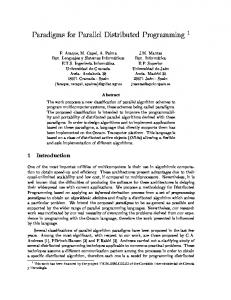
The PPE contains a 64-bit general purpose register set, a 64-bit floating point register set, and a 128-bit vector register set. This main core is designed to run the operating system and manage the devices. Each SPE consists of a Synergistic Processing Unit (SPU) along with a memory flow controller (MFC) which acts as an interface between the SPU and the EIB. The SPU has a processing unit and a Local Store (LS) of 256 KB. Programs running on an SPE reside in its LS and perform computation on the data present in the LS. Each SPU contains 128 general purpose 128-bit vector registers, making it a SIMD processing unit. SPEs do not have direct access to the system’s main memory, and to enable data flow between the main memory and the LS of a SPE, explicit DMA transfers need to be carried out. Each core runs its own individual thread. A block diagram of an SPE is shown in Figure 1.2. Each SPE has two instruction pipelines – even and odd, providing instruction level parallelism: Certain instructions, like floating point operations, integer operations, logical and byte instructions, are scheduled to the even pipeline, and other instructions, like load and store, branching operations, are scheduled to the odd pipeline. The Cell BE has been the main processor in Sony PlayStation 3. On this system, six SPEs are available for computations and can be used for scientific computing [21]. The IBM QS20, and QS22 with PowerXCell 8i processors, Cell blades provide two 3.2 GHz Cell processors, based on the SMP (Symmetric Multi-Processing) architecture. The EIB is extended across the two Cell processors through a high speed coherent interface, which enables a transparent access to a total of 16 SPEs by the programs running on the Cell blade. Due to their physical locations, the on-chip communication latency between two components of a single Cell processor is lower than the off-chip communication between two components on the two separate processors on a Cell blade.
4 Even
Odd
FP, int, logical, byte
L/S, byte, branch
Local Store 256 KB
128 x 128b Reg.
DMA I/O
MMU
EIB
Figure 1.2: Block diagram of a Synergistic Processing Element of the Cell processor, showing the 128-bit register set, 256 KB Local Store, even and odd instruction pipelines, and the DMA I/O controller with the memory management unit (MMU). The DMA I/O provides an interface to the Element Interconnect Bus (EIB).
1.2.1.1
Challenges on the Cell Processor
The SPEs are designed for compute intensive processing in parallel, while the PPE takes care of the management. There are numerous constraints and restrictions which make development of optimized applications on the Cell processor quite challenging. The SPEs are designed for SIMD computation and do not comparatively perform well on scalar data. A major limiting factor is the small Local Store of 256 KB where the SPE code and all data has to reside along with stack and heap memory used during execution. This calls for implementations which use as little memory as possible on the SPEs. Moreover, no memory protection is provided and the developer needs to take care of the memory management. Data are transferred from the main memory through DMA transfers explicitly. DMA transfers of only 1, 2, 4, 8, 16 or multiples of 16 bytes are allowed, and the source and destination address of the data being transferred should be aligned at 16-byte boundary for 16 byte or larger data size, and naturally aligned for smaller sizes. Optimal performance is achieved when DMA transfers are multiples of 128 byte sized and aligned to the cache line, which is 128 byte boundaries. Further, DMA transfer latency from the main memory of the system is high, and to achieve efficiency on this processor, such transfers should be minimized. These DMA transfers are non-blocking, and a performance improvement can be realized by overlapping computations with DMA transfers while using double buffering. 1.2.2
Graphics Processors
Graphics Processing Units (GPUs) are massively parallel multi-threaded architectures, providing hundreds of cores. They are, therefore, aptly referred to as many-core processors. They are specialized processors, primarily designed to perform compute-intensive graphics render-
5 ing, off-loaded from the system’s main CPU. Their highly parallel architecture makes them more powerful for a range of complex processing than a general-purpose CPU, and hence, GPUs have been increasingly employed in performing intensive computations for problems taken from numerous areas of computing, and not just graphics, in a technique commonly termed as General-Purpose Computing on Graphics Processing Units (GPGPU). GPUs are developed by a number of companies, mainly NVIDIA, Intel, and AMD/ATI. In the rest of the discussion, we will assume NVIDIA GPU architecture [72, 84], although the GPUs manufactured by other companies are not very different conceptually. The computational cores on a GPU are grouped into a hierarchy. A particular NVIDIA GPU consists of a number of Streaming Multiprocessors (SM), also referred to as simply multiprocessors. Each such multiprocessor is made up of a number of scalar computing cores, called Streaming Processors (SPs). A GPU system is equipped with an off-chip memory, which can be directly accessed by all threads running on the GPU. Each SM has a small shared memory, which can be accessed only by threads running on the particular SM. GPUs are primarily designed for graphics processing, and are therefore, very restrictive in terms of offered operations and programmability. NVIDIA developed a computational model unifying the GPU architecture with general-purpose programming concepts, called Compute Unified Device Architecture, or CUDA [32]. It also provides an API for easy programmability of the NVIDIA GPUs. Apart from the CUDA API, many other APIs also exist, such as OpenCL [56], Microsoft’s DirectCompute [30], and BrookGPU [75], and they all provide integration with the CUDA API. CUDA enables fine-grained and scalable parallelism by defining the computational parallelism in terms of tasks and threads. A computational problem is divided into coarse-grained tasks, called CUDA thread blocks, each further divided into fine-grained threads. Threads in a thread block may cooperate with each other to compute the corresponding task. A CUDA kernel is a computational function which is executed in parallel by the CUDA threads. A kernel defines the thread blocks, forming a one or two-dimensional grid. Each thread block is defined as a one, two or three-dimensional array of threads. A kernel defines the computation of such a thread, and all the threads perform the computation in parallel, following the Single-Instruction Multiple-Thread (SIMT) architecture. CUDA maps the kernel grid onto the GPU as follows: scheduling granularity is at the level of thread blocks, where each thread block is scheduled to one SM. A conceptual diagram of the CUDA architecture mapping on to the GPU is shown in Fig. 1.3. A particular SM may have multiple thread blocks assigned to it simultaneously, as permitted by the resources available on the SM. The execution of a thread block is assumed to be independent of all other thread blocks, and may be executed in any order. As we mentioned above, the system memory space is defined as a hierarchy: The off-chip device memory is accessible by every thread in a grid, the shared memory available on each
SP SP SP SP SP SP SP SP Shared Memory
SM
Device Memory
6
0,0 1,0 2,0 0,1 1,1 2,1
0,0 1,0 2,0 0,1 1,1 2,1
0,2 1,2 2,2
0,2 1,2 2,2
0,3 1,3 2,3
Grid GPU
Thread Block
Figure 1.3: A conceptual block diagram of the CUDA architecture mapping to a GPU. On the left is a GPU architecture, with multiprocessors (SM), each containing scalar processors (SPs) and shared memory. All the multiprocessors have access to the off-chip device memory. On the right is the CUDA architecture, where a kernel is decomposed as a grid, containing CUDA thread blocks. An example mapping (center arrows) of the thread blocks onto the SMs is shown, where, all thread blocks in each of the row in the grid are mapped to one SM.
SM is accessible by all threads in a particular thread block executing on that SM, and has the lifetime of the corresponding thread block. The shared memory is partitioned among all the thread blocks assigned to the SM. Threads in a block are scheduled for execution on an SM as warps, which are groups of 32 threads. A set of registers available on an SM is partitioned among all the warps on the SM. The shared memory, being on-chip, and physically very close to the computing cores in an SM, have a low latency, but are small in size (16 KB in most GPUs). The device memory is large, but being off-chip, has a high access latency. Compared to the access latency of the main memory in a general-purpose CPU, that of the device memory on GPU is higher due to lack of any caches on the chip. 1.2.2.1
Challenges on a GPU
Being a specialized architecture, with massive SIMT parallelism, graphics processors pose numerous challenges in order to harness their computational power. Since threads are scheduled on an SM as warps, having multiple warps scheduled on an SM is beneficial for performance since it hides instruction and memory latencies during the execution. Thread blocks defined as a multiple of the warp-size minimize resource wastage, and also, if there are p SMs on a GPU, we want the total number of thread blocks in the grid to be in excess of p to take advantage of the parallelism. A large number of thread blocks also ensures a better load balance among the SMs. We term the total number of thread blocks in a grid as degree of parallelism. The amount of shared memory usage by a kernel puts a constraint on the number of thread blocks that can be scheduled on an SM simultaneously, since the shared memory is partitioned among the corresponding thread blocks. A similar constraint is also established due to the limited number of registers available on an SM, which are partitioned among the corresponding warps.
7 Contiguous memory accesses by threads in a warp from the device memory enables memory coalescing, reducing the memory transactions to be carried out, and thereby, improving the performance. Moreover, since the access latency to the device memory is high, the limited amount of shared memory needs to be effectively used to minimize memory access from the device memory. CUDA also puts forth limitations on the maximum thread block size that can be created: A maximum of 512 threads are allowed in a block. 1.2.3
Algorithms and Applications on Emerging Architectures
The emerging heterogeneous and homogeneous multi/many-core architectures provide a wide variety of architectural features which make them suitable for high-performance computing. Even though the graphics processors generally offer the highest theoretical computational power, due to their specialized design, they are more suited to highly parallel stream processing, and may not perform well with certain coarse-grained parallel computations where the Cell processor, or general-purpose CPUs will perform better. GPUs are designed to be used as a co-processing device where the host CPU and the GPU share the computational loads, depending on which tasks are better suited to either processor, as a heterogeneous computing system. Similarly even though being a stand-alone processor, the Cell BE may also be integrated with a CPU, or even a GPU, to share the computations. Roadrunner [13], a supercomputer which topped the top500 list [105] in June 2008 as world’s first petaflop system is built on such a heterogeneous/hybrid design, where the PowerXCell 8i processors are attached to dual-core AMD Opteron processors. These emerging multi/many-core architectures are increasingly being used for high performance computing. The Cell Broadband Engine and graphics processors, due to their unique designs and high computational power, have been the main target for general purpose computing to accelerate computations in various scientific applications [69, 25, 84]. Algorithms have been developed on these architectures for various fundamental problems, for example sorting [50, 76, 96], number crunching problems like fast fourier transforms [9, 53], random number generators [11, 63], and irregular problems like list ranking [10, 87]. Researchers have also targeted accelerating specific applications on the Cell BE and graphics processors, taken from numerous areas of computing, for instance, pattern matching [97], video encoding/decoding [12], financial modeling [2], and bioinformatics [91]. There has been a significant interest in porting bioinformatics applications to the Cell and GPUs. Sachdeva et al. [91] evaluated the performance of a basic porting of FASTA and ClustalW applications on to the Cell platform. ClustalW is a multiple sequence alignment application which leverages on using pairwise sequence alignment algorithms, such as local alignment, multiple times. An architecture-aware implementation of this application, tuned to the Cell processor, was developed by Vandierendonck et al. [108]. Farrar [43] developed a Cell-based SIMD vectorized implementation of the Smith-Waterman [103] local sequence
8 alignment algorithm. Manavski et al. [78] implemented this local alignment algorithm on GPUs. Blagojevic et al. [19] and Charalambous et al. [24] implemented RAxML on the Cell and graphics processor, respectively, an application for inferring large phylogenetic trees. Many other researchers have also implemented parallel algorithms for sequence alignments on these architectures [112, 113, 3, 68]. In our work, we look at the fundamental problem of pairwise genomic alignments, and develop efficient parallel algorithms for an architecture like the Cell processor. Apart from this, we also look at certain other applications involving pairwise computations, taken from systems biology, fluid dynamics and systems biology. There has also been some interest in executing pairwise computations on the emerging architectures. Arora et al. [6] demonstrate the all-pairs N -body computational kernels on various multi-core platforms, including the Cell processor and NVIDIA graphics processors. Acceleration of the pairwise distance matrix computation employed in multiple sequence alignment algorithms was demonstrated on the Cell processor by Wirawan et al. [114]. Also, Barrachina et al. [15] explored graphics processors for matrix multiplication on dense matrices, and Bell et al. [23] for sparse matrices. 1.2.4
Contributions on the Emerging Architectures Paradigm
On the platform of emerging architectures, we develop efficient parallel techniques for various kinds of pairwise computations on the multi- and many-core processors. First, we develop a hybrid parallel algorithm on the Cell platform to compute an optimal alignment of two input genomic sequences (Chapter 2). This algorithm is built upon the wavefront communication scheme which was first proposed by Edmiston et al. [40], and a parallel-prefix based pairwise sequence alignment algorithm proposed by Aluru et al. [5]. This algorithm works in linear space, in the light of the limited on-chip memories on the cores of the Cell processor. We apply our algorithm to various genomic alignments – global/local, spliced and syntenic. Next, we look at the abstract problem of pairwise computations for a number of input entities (Chapter 3). We develop methods to efficiently schedule such pairwise computations on the Cell processor and graphics processors. On the Cell processor, our scheme optimizes the performance by minimizing the total number of DMA transfers required. We apply our implementation on the Cell to applications taken from the areas of systems biology, materials science and fluid dynamics. We develop a software library, TINGe-CBE, for inference of genomewide gene regulatory networks from microarray data, on the Cell platform. Next, we develop a generalized all-pairs computations library, libpnorm, with in-built Lp -norm distance metric computational kernel for all-pairs computations. Such computations are applied in materials science, to construct stochastic models of properties for a given set of heterogeneous media, and in fluid dynamics to discover coherent structures in the design of flapping-wing Micro Air Vehicles.
9 On graphics processors, we develop an efficient scheme to perform such pairwise computations, where the shared memory on the SMs is employed to reduce the number of accesses to the device memory. We implement our scheme as a generalized library, libpairwise, on the GPU platform. We use it to conduct an in-depth analysis of the effects on the performance based on a choice of various parameters used in our scheme, and demonstrate how to choose these parameters to maximize the performance. Furthermore, we compare the performance of our schemes on the Cell and graphics processors, with multi-core parallelizations on a generalpurpose CPU.
1.3
Parallel Processing with Cloud Computing
A cloud represents a set of computing resources, which are provided to a user in an abstract manner. Conceptually, cloud computing is considered as a paradigm shift towards the server-client system, where all the details of the computing resources and system management are abstracted away from the user. A user does not need to have any knowledge of the system infrastructure details, and parallelism involved in the cloud. One of the main motivations behind such a computing paradigm is simplicity. It involves development of broadly applicable high level abstractions as a means to deliver easy programmability and cyber resources to the user, while hiding complexities of system architecture, parallelism and algorithms, heterogeneity, and fault-tolerance. A cloud-based system provides a very simple interface to the user, which is general enough to enable realization of many different applications while providing some performance guarantees. With this interface (also called application programming interface, or API), a user writes an application with minimal complexity. A cloud may provide any kind of computing resource, ranging from a sequential processor to a large parallel cluster of high-performance processors, possibly distributed across the planet. This concept is visualized in Figure 1.4. The continuing explosive growth in raw data in virtually every sphere of human activity necessitates large scale data-intensive and compute-intensive processing. While such processing often requires the use of distributed/parallel systems to handle memory, storage and run-time needs, developing applications from scratch for such platforms is expensive and cumbersome enough to prevent their widespread use. A cloud computing based framework is helpful in addressing this problem since an application writer (user) needs to focus only on the crux of the computations and does not need to worry about the system details. However, a major challenge in designing such a cloud computing framework for scientific computing is the abstraction of the computational patterns in the targeted applications. Following data-parallel computing model, the processing on a given set of input data can be defined as independent computations which can be performed in parallel. Google’s MapReduce paradigm [37] is one such example, and its recent prominence has renewed interest in development of such abstractions. In the following we describe the MapReduce paradigm in brief.
10
Servers & Compute Nodes
Storage & Databases
Cloud Application Server & Algorithms
API
API
User
User
API
API
User
User
Figure 1.4: A conceptual diagram of Cloud computing. The computing, storage and management resources reside in a cloud, and a user is oblivious to the details of the system infrastructure and algorithms. The users make use of the resources through an application programming interface (API) provided by the cloud. The API is very simple for the users to write their applications without the knowledge of the internal parallelism and complexities in the cloud.
1.3.1
MapReduce Paradigm
Google’s MapReduce paradigm [37], first proposed in 2004, borrows the concepts of map and reduce functions which are commonly used in functional programming. This framework provides two functions: Map and Reduce, for a user to define in order to realize an application. Both these functions are defined on data represented as key-value pairs. Map takes such data from one domain and maps to data in another intermediate domain: map(k1 , v1 ) −→ list(k2 , v2 ), where a data entity (k1 , v1 ) is mapped to a set of data entities as list(k2 , v2 ). The subscripts 1
and
2
for the data represent different domains. Reduce function takes a set of data from the
intermediate domain, corresponding to the same keys, and generates a set of values in another domain: reduce(k2 , list(v2 )) −→ list(v3 ). Once these two functions are defined by a user, the system executes them in a massively parallel manner. With these two simple functions, the MapReduce framework provides a versatile way to solve numerous data-parallel applications through innovative use of these user-specified
11 Map and Reduce functions. Since its introduction, apart from its use internally at Google, applications of MapReduce framework are being investigated in multiple fields (for example, see [106] and the NSF Cluster Exploratory (CluE) program [45]). 1.3.2
Applications on MapReduce
Major large-scale MapReduce framework based system implementations include the implementation used at Google [37], and the open-source Apache Hadoop project [18]. Various other implementations of MapReduce also exist, such as Phoenix [86] – a shared-memory implementation, Mars [60] – an implementation on graphics processors, and an implementation on the Cell BE platform [36]. QtConcurrent [1] is another implementation of MapReduce as a C++ template library for the shared-memory platform. BashReduce [46] provides MapReduce written as bash scripting. The MapReduce framework is used in a wide range of data-parallel applications, such as distributed grep, distributed sort, web link-graph/link-list reversal, inverted-index construction, and document clustering. Researchers have also adapted and enhanced the basic MapReduce framework to address more specific data processing domains, like relational data queries [115], machine learning on multi-cores [26], and .NET-based distributed computing [66]. Such functional style programming models with high level abstractions are important for the success of cloud computing, as the goal is to provide vast computing and storage resources to the user without knowledge of architecture, parallelism or data location within the cloud. 1.3.3
Contributions on the Cloud Computing Paradigm
Despite its success, MapReduce can only abstract independent data-parallel processing of individual data entities, where data dependencies are not involved. Numerous data and compute intensive applications do not fit this simple model. A particularly important class of applications outside the scope of MapReduce framework involve trees – a diverse class of data structures pervasively used in nearly all areas of computing. Tree-based applications involving large-scale data-intensive processing need to be carried out on distributed/parallel computers and/or storage systems. Moreover the processing of data at a particular node of the tree may require the data from some other nodes in the tree, creating data dependencies. Structured documents represented using markup languages, such as SGML and its derivatives such as XML, have a tree based representation. Vast amounts of archives of such documents need sophisticated query processing, and can be efficiently performed by exploiting their tree structure. Skillicorn [102] models operations on such structured text using parameterized tree homomorphism functions on binary trees. Spatial trees [92] have applications in geometric modeling, graphics and image processing [35]. Data-intensive tree-based applications abound in high-performance scientific computing, both for maintaining and mining scientific data sets
12 such as the Sloan Digital Sky Survey [104], and in applications such as N -body simulations [111, 39, 14], molecular dynamics [20], and computational electromagnetics [59]. Tree-based data and compute intensive applications require significant programming effort by the user, particularly when dealing with large trees in a distributed/parallel environment. A MapReduce style abstraction for tree structures can be beneficial, albeit more challenging due to the variety of tree data structures and algorithmic techniques designed for trees. In our work, we propose a general framework for computations on tree structures in Chapter 4. Our framework involves two user-specified functions that can be crafted in numerous ways to realize widely used operations on tree structures. These functions are based on the fundamental parent-children relationships common to all tree data structures, while relegating storage schema, algorithms, parallelism and concurrency issues to the framework. We report on a detailed implementation of the framework, as a generic programming library – TreeWorks, and demonstrate its applicability by developing two applications – all k-nearest neighbors and Fast Multipole Method (FMM) based simulations – by merely defining the two user-specified functions of the framework in various ways, and let the framework handle the rest.
13
CHAPTER 2.
GENOMIC ALIGNMENTS ON HETEROGENEOUS MULTI-CORE PROCESSORS
Genomic alignments, as a means to uncover evolutionary relationships among organisms, are a fundamental tool in computational biology. In this chapter, we present a comprehensive study of developing parallel algorithms for genomic alignments on the Cell, exploiting its thread and data level parallelism. First, we develop a parallel implementation on the Cell that computes optimal alignments and adopts Hirschberg’s linear space technique. The former is essential as merely computing optimal alignment scores is not useful, while the latter is needed to permit alignments of longer sequences. We then present Cell implementations of two advanced alignment techniques – spliced alignments and syntenic alignments. Spliced alignments are useful in aligning mRNA sequences with corresponding genomic sequences to uncover the gene structure. Syntenic alignments are used to discover conserved exons and other sequences between long genomic sequences from different organisms. We present experimental results for these three types of alignments on 16 SPE cores of the IBM QS20 dual-Cell blade system.
2.1
Genomic Alignments
Alignment algorithms enable discovery of evolutionary relationships among biological sequences, and arise in many contexts and applications in computational biology. Over the past two decades, a number of alignment algorithms have been developed to elucidate different types of sequence relationships of interest. The most common types of alignments are the global alignments [82] which correspond to aligning sequences in their entirety, and local alignments [103] which correspond to aligning sequences that each contain a substring which are highly similar. Some applications require more complex alignment strategies. One such example is when aligning an mRNA sequence transcribed from a eukaryotic gene with the corresponding genomic sequence to infer the gene structure [51]. A gene consists of alternating regions called exons and introns, while the transcribed mRNA corresponds to a concatenated sequence of the exons. This requires identifying a partition of the mRNA sequence into consecutive substrings (the exons) which align to the same number of ordered, non-overlapping, non-consecutive substrings of the gene, a problem known as spliced alignment. Another important problem is that of syntenic alignment [65], for aligning two sequences that contain conserved substrings
14
S1
S1 S2
S2 (a) Global Alignment
(b) Local Alignment
S1
S1
S2 (c) Spliced Alignment
S2 (d) Syntenic Alignment
Figure 2.1: Genomic alignments: the thick portions of sequences S1 and S2 show the segments which are aligned. (a) Global Alignment: Both sequences are aligned in their entirety. (b) Local Alignment: A substring from each sequence are aligned. (c) Spliced Alignment: Ordered series of substrings of one sequence are aligned to the entire second sequence. (d) Syntenic Alignment: Ordered series of substrings of one sequence are aligned with ordered series of substrings on the second sequence. For (b), (c) and (d), the goal includes finding the aligning regions such that the score of the resulting alignment, as given by a score function, is maximized. Both the number and boundaries of aligning regions are unknown and need to be inferred by the algorithm. Only the sequences S1 and S2 are the input for each alignment problem.
that occur in the same order (such as genes with conserved exons from different organisms, or long syntenic regions between genomes of two organisms). An illustration of global alignment, spliced alignment and syntenic alignment is shown in Figure 2.1. These alignment problems can be solved using dynamic programming, and a number of algorithms exist to do so [82, 103, 51, 65]. The computation time required by these algorithms is proportional to the product of the lengths of the two input sequences1 . The dynamic programming algorithms use a constant number of dynamic programming tables of quadratic size. To enable alignment between larger sequences, Hirschberg’s space saving strategy [62] can be applied in conjunction with most of these algorithms to obtain linear space complexity. Several algorithms have also been developed to solve these problems in parallel [90, 42, 5, 40, 47]. Some of these parallelize the computations within a single processor utilizing its vector processing units and SIMD-style instructions [90, 42]. Other algorithms deal with parallelization across multiple processors. Of these, the two most prominent parallelization strategies are the diagonal wavefront parallelization by Edmiston et al. [40], and the row-wise parallel prefix based parallelization algorithm by Aluru et al. [5, 47]. As we mentioned in the introduction, recently many researchers have ported various bioin1 Although [51] presents an algorithm with cubic complexity, the spliced alignment problem can be treated as a special case of syntenic alignment and solved in quadratic time, as will be shown later; also, the original Smith-Waterman algorithm [103] has cubic complexity, but it is widely known that this can be implemented in quadratic time, for example see [4].
15 formatics applications to the Cell platform [91, 19, 108, 112, 3]. Many of these applications deal with pairwise genomic alignments [91, 112, 3]. These current methods for sequence alignments on the Cell are restricted to the basic Smith-Waterman algorithm [103] for local alignments. Some researchers have also implemented the local alignment algorithm in parallel using Edmiston’s wavefront pattern on the Cell [113, 3]. All of these implementations compute only the optimal score of the alignment in parallel, and not an actual alignment. Scoring is merely a measure to assess the alignment quality, and an actual alignment with the optimal score is what is needed. While most Cell implementations have ignored this issue, Aji et al. [3] also produce an actual alignment. However, they use the standard sequential traceback algorithm to produce an optimal alignment, and use the multi-core processing units only for the purpose of computing the dynamic programming table. All these current implementations have quadratic memory usage since they store the whole dynamic programming table in the memory. Because of this, most of these are limited to small input sequence sizes. Our aim in this work is to develop a Cell implementation for sequence alignments to overcome all these limitations: We develop a hybrid parallel genomic sequence alignment algorithm combining the parallelization strategies from Aluru et al. [5] and Edmiston et al. [40] in order to efficiently use the power of the Cell processor and describe it in Section 2.2. We also provide a communication complexity model for the Cell to show that this hybrid scheme results in fewer number of DMA transfers; We incorporate Hirschberg’s space-saving technique [62, 81] to compute alignments in linear space, which is important in light of limited memory available per SPE and the high costs of data transfers to/from the main memory; We produce actual alignments using our approach, which is important to gain more biological insight into the genomic sequences begin aligned; In addition to the basic global/local alignment, we apply this scheme to the more advanced spliced and syntenic alignment problems in Sections 2.3 and 2.4, and analyze their scaling to two Cell processors on the IBM QS20 Cell blade.
2.2
Global/Local Alignment
Consider two sequences S1 = a1 a2 . . . am and S2 = b1 b2 . . . bn over the alphabet Σ, and let ‘−’ denote the gap character. A global alignment of the two sequences is a 2 × N matrix, where
N ≥ max(m, n), such that each row represents one of the sequences with gaps inserted in
certain positions and no column contains gaps in both sequences. The alignment is scored as
follows: a function, score : Σ × Σ → R, prescribes the score for any column in the alignment that does not contain a gap. Scores of columns involving gaps are determined by an affine gap penalty function: for a maximal consecutive sequence of k gaps, a penalty of h + gk is applied. Thus, the first gap in a maximal sequence is charged h + g, while the rest of the gaps are charged g each. When h = 0, the scoring function is called a constant gap penalty function. The score of the alignment is the sum of scores over all the columns. Affine gap penalty functions are commonly used so that a sequence of gaps is assigned less penalty than
16 treating them as individual gaps – this is because a mutation affecting a short substring is more likely than several individual point mutations. The global alignment problem with affine gap penalty function can be solved by using three (m + 1) × (n + 1) sized dynamic programming tables, denoted C, D (for deletion) and I (for insertion) in the following. An element [i, j] in a table is used to store the optimal score of an
alignment between a1 a2 . . . ai and b1 b2 . . . bj with the following restrictions on the last column of the alignment: ai is matched with bj in C, a gap is matched with bj in D, and ai is matched with a gap in I. The tables can be computed using the following recursive equations, which can be applied row by row, column by column, or antidiagonal by antidiagonal (also called minor diagonal) once the top row and leftmost column of each table are initialized: C[i − 1, j − 1] C[i, j] = score(ai , bj ) + max D[i − 1, j − 1] I[i − 1, j − 1] C[i, j − 1] − (h + g) D[i, j] = max D[i, j − 1] − g I[i, j − 1] − (h + g) C[i − 1, j] − (h + g) I[i, j] = max D[i − 1, j] − (h + g) I[i − 1, j] − g
(2.1)
(2.2)
(2.3)
After the tables are computed, the maximum of the scores in the bottom right entries of the three tables gives the optimal alignment score. By keeping track of a pointer from each entry to one of the entries that resulted in the maximum while computing its score, an optimal alignment can be constructed by retracing the pointers from bottom right to the top left corner. 2.2.1
Reducing Memory Usage
The algorithm takes O(mn) time and O(mn) space. The space can be reduced to O(m + n) using Hirschberg’s technique [62, 81]. This method is a recursive technique to compute the alignments and the scores. The recursion is based on the fact that if the optimal alignment is divided into two, the resulting parts will each be the optimal alignments of the corresponding segments of the sequences. The basic technique is given in Algorithm 1. In this scheme, one of the input sequences is divided into two halves, and tables are computed for each half aligned with the other input sequence. This is done in the normal top down and left to right fashion for the upper half and in a reverse bottom up and right to left manner (aligning the reverses of the input sequences) for the lower half. Since for computation of the entry (i, j), only the entries in previous row i − 1 and previous column j − 1 are required, it is sufficient to store a linear array for the last computed row. Once the middle two rows are ob-
17 Algorithm 1: space saving align(S10 , S20 ) – Computing an optimal alignment of two sequences, S10 and S20 of lengths m0 and n0 , respectively, in linear space using Hirschberg’s recursive space saving technique. 1 2 3 4 5 6 7
8
9
10 11 12
m0 ← length(S10 ); n0 ← length(S20 ); return if m0 = 0 and n0 = 0; 0 S100 ← substring S10 [0 · · · m2 − 1]; 0 rev S100 ← reverse of substring S10 [ m2 · · · m0 − 1]; rev S20 ← reverse of S20 ; compute alignment scores for S100 and S20 , storing only the last computed row, to 0 obtain the middle row m2 − 1; compute alignment scores for rev S100 and rev S20 , storing only the last computed 0 row, to obtain the middle row m2 ; 0 0 scan the scores in the obtained rows m2 − 1 and m2 , to find an optimal score, and store the corresponding alignment information; i ← position in the rows corresponding to an optimal score; space saving align(S100 , S20 [0 · · · i − 1]); 0 space saving align(S10 [ m2 · · · m0 − 1], S20 [i · · · n0 − 1]);
tained from the corresponding two halves, they are combined to obtain the optimal alignment score, dividing the second sequence at the appropriate place where the optimal alignment path crosses these middle rows. Care needs to be taken to handle the gap continuations across the division, and the possibility of multiple optimal alignment paths. The problem is hence divided into two subproblems and this is repeated recursively for each subproblem. An illustration of recursion using this scheme is shown in Figure 2.2. 2.2.2
Space-Efficient Global Alignment on CBE
Our parallel alignment algorithm on the CBE [93, 94] is a combination of the wavefront communication pattern of the algorithm by Edmiston et al. [40], with the parallel-prefix based space-saving parallel algorithm by Aluru et al. [5]. Both algorithms compute an optimal alignment of the input sequences. In the wavefront method, each table is divided into a p × p
matrix of blocks where p is the number of processors. Each processor is assigned a column of blocks. The blocks are collectively computed one antidiagonal at a time (see Figure 2.3). All blocks on an antidiagonal can be computed simultaneously as they depend only on blocks on the previous two antidiagonals. Because of block assignment to processors, each processor only needs to receive the last column of a block (plus an additional element) from the previous processor. The parallel prefix based algorithm computes each row of the tables in parallel. One of the
18
Optimal Alignment Path
Figure 2.2: Hirschberg’s sequential recursive space saving scheme. The whole problem is recursively divided into subproblems around an optimal alignment path, while using linear space. The middle two rows are enlarged for the first recursion showing an example of an optimal alignment path crossing them (not shown for subsequent divisions). The four bold arrows show the direction of computations for the two halves.
sequences is provided to all the processors and the other is equally divided among them — each processor hence receives a block of columns. The intersections of the optimal alignment path with the last column in each block (called special columns) define the segment of the first sequence to be used within a particular processor independently of other blocks. These are computed row-wise using parallel prefix operations. The idea is visualized in Figure 2.4. Once the problem is divided among the processors, each processor performs a sequential alignment on its local segments of sequences using Hirschberg’s technique, and the results from all processors are concatenated to yield the actual alignment. To derive an efficient parallel implementation on the Cell, we combine the wavefront technique with the space-saving special columns technique of the parallel prefix based approach to obtain a hybrid parallel algorithm. In the wavefront scheme, each computing unit works on a block of the tables independently, communicating the last column(s) to the next processor when done and then starts computation on the next block; the parallel prefix approach requires the computing units to communicate a single element when computing each row. Short but frequent communications for each row increase channel stalls in the SPEs which is reduced to one bulk communication per block in the wavefront scheme. Each communication leads to a synchronization point and, to make most use of parallelism, such points should be minimized. Moreover, the block size can be optimized for DMA transfer which makes it a better choice for the Cell Broadband Engine. A more detailed communication complexity analysis for the Cell processor is given in the next subsection. Our implementation provides efficient space usage along with traceback capability. Adopting the space-saving method is particularly important for the CBE, as each SPE has access to only 256 KB of local store memory. Thus, our implementation significantly extends the scale of alignments compared to previous works on CBE
19
SPE0
SPE1 SPE2
SPE3 SPE4
Figure 2.3: Block division in wavefront technique. Each processor is assigned a column of blocks, as indicated by the processor label inside each block. Block computations follow diagonal wavefront pattern (the blocks in the same shade of gray are computed simultaneously in parallel). The shaded rightmost column of each computation block of the table needs to be sent to the next processor for computing its assigned block in the next iteration.
which require storing the entire matrix. We partition each dynamic programming table into blocks of size r × np . The number of
rows in a block, r, is chosen so as to optimize DMA transfers (a multiple of 128 bytes). Each
row of blocks contains as many blocks as SPEs. Each column of blocks is assigned to a single SPE. We modify the parallel space-saving algorithm [5] to incorporate the wavefront technique and store only the last columns (special columns) for each SPE block. This enables the use of double buffering in moving input column sequence and overlapping of DMA transfers with block computations. Each SPE transfers portions of the second sequence allotted to it by the PPE. For each computation block, it transfers blocks of first sequence using double buffering and performs the table computations in linear space, while storing all of the last column. Once done, it transfers the recently computed block of last column data to the next SPE and continues computation on the next block. This scheme for SPE q (with total of p SPEs) is shown as pseudo-code in Algorithm 2. This part of the algorithm is called the problem decomposition phase. Once the special columns are computed containing pointers to the previous special columns as described in [5], the segments of the first sequence are found which are to be aligned to the segments of the second sequence on the corresponding SPEs. This is followed by the sequential version of Hirschberg’s space-saving technique based algorithm, where each SPE simultaneously computes optimal alignments for its local subproblem. On completion, each SPE writes its portion of alignment to the main memory through DMA transfers, which are then concatenated to obtain the overall alignment.
20
Optimal Alignment Path
SPE0
SPE1 SPE2
SPE3 SPE4
Figure 2.4: Block division in the parallel prefix based technique. The second sequence is divided into vertical blocks, which are assigned to different processors Pi . Special columns constitute the shaded rightmost column of each vertical block and the dotted circles show intersection of an optimal alignment path with the special columns, which are used for problem division. The shaded rectangles around the optimal alignment path represent the subdivisions of the problem for each processor.
2.2.3
Analyzing Communication Complexity on the Cell BE
In this section, we provide an analysis of the algorithm complexity on the Cell Broadband Engine. Since the computational complexity is the same for the standard wavefront method, the parallel prefix based method, and our hybrid scheme, we only focus on communication, which arises from DMA transfers between different components on the Cell processor. Our hybrid algorithm performs the same number of DMA transfers as current wavefront implementations, all of which use quadratic space and cannot compute the alignment itself in parallel. Thus, we provide linear space usage and parallel computation of alignment on SPEs without incurring any additional DMA transfers. While this is achieved by borrowing these features from the parallel prefix based algorithm, we show that a direct Cell implementation of that algorithm is inferior and causes an increase in the number of DMA transfers. Bader et al. [9] have given a complexity model for the Cell processor in which the algorithmic complexity is represented with three terms: the computation complexity, number of DMA transfers, and number of branching operations in the SPEs. They only consider the number of DMA transfers to measure the communication complexity. We provide a more detailed communication complexity analysis by taking into account various latencies for DMA transfers. Based on the communication network analysis for the Cell processor given in [73], we model the communication complexity with the number of DMA transfers, their latencies, and the size of data being transferred. We do not consider mailboxes and signal notifications as their latencies are almost constant since they involve only a small constant number of bytes, and are very small when compared to DMA transfer latencies.
21
Algorithm 2: Problem decomposition phase of the parallel space-saving algorithm for SPE q. BLOCKSIZE is equal to the number of rows r in a block. 1 2 3 4 5 6 7 8 9 10 11 12 13 14 15 16 17 18 19 20 21 22 23
24
m0 ← length(S10 ); n0 ← length(S20 ); start DMA transfer of S20 , the allocated S2 segment for SPE q; m0 num blocks ← BLOCKSIZE ; start DMA transfer of curr block, the substring S10 [0 · · · BLOCKSIZE − 1]; for k ← 1 to num blocks − 1 do if q 6= 0 then receive signal from SPE q − 1 end start DMA transfer of next block, the next BLOCKSIZE characters of S10 ; wait for completion of curr block transfer; for i ← 1 to BLOCKSIZE do compute entries of row i for three tables re-using single row buffer; special col[i] ← last entry in row i; end if q 6= p − 1 then DMA transfer last computed block of special col to next SPE q + 1; signal the next SPE q + 1 that its first column has been written; end curr block ← next block; end wait for completion of curr block transfer; perform linear space table computation on curr block storing the last column in special col array; DMA transfer last block of computed special col to next SPE;
On the Cell processor, there are four basic types of explicit DMA transfers based on the source and destination of the data being transferred. All transfers are stated from the perspective of an SPE. SPEs use specific commands to transfer data through DMA. There are two sets of such commands: gets – transfer data into the SPE’s local store (LS); puts – transfer data out from the SPE’s local store. This gives us the four types of DMA transfers: 1. from the LS of an SPE to the main memory (puts), 2. to the LS of an SPE from the main memory (gets), 3. from the LS of an SPE to the LS of another SPE (puts), and, 4. to the LS of an SPE from the LS of another SPE (gets).
22 The gets and puts commands for transfers to/from an SPE’s LS from/to the LS of another SPE have approximately the same latencies, so we only consider the puts commands for interSPE data transfers. We use some basic observations taken from [73] to describe our model. The latency for the process of DMA transfer, initiated by an SPE, can be broadly divided into two phases: (1) flow-through latency (τ ), which includes the process starting from the DMA command issue by the SPE till the bus request is sent to the Element Interconnect Bus (EIB) – this is typically 30 to 50 cycles; (2) transfer latency (µ), when the data is actually transferred through the EIB. The latencies for puts to main memory and puts to local store are almost the same. This is because the puts command is considered complete when the data is transferred to the memory interface controller (MIC) on the Cell processor and does not include the latency to transfer it all the way to the main memory. The latencies for gets from main memory are higher since it includes the off-chip data transfer latency from the main memory to the MIC, and the latency to transfer data from MIC to the LS of the SPE. We denote these latencies as follows: 1. τl – flow-through latency for puts and gets to/from LS and puts to main memory. 2. µl – transfer latency for puts and gets to/from LS and puts to main memory. 3. τm – flow-through latency for gets from main memory. 4. µm – transfer latency for gets from main memory. Therefore, the total time required for one DMA transfer of b bytes from the main memory to the local store of an SPE is τm + bµm , and the time of DMA transfer of b bytes from local store of one SPE to local store of another SPE is τl + bµl . We now use this model to analyze the communication complexity of our hybrid scheme. Initially we divide the second sequence (of length n) equally among all p processing units (the number of SPEs), giving substrings of length
n p
to each SPE. Next we divide the first sequence
into segments of size B, to obtain blocks of sizes B × np . Therefore, a single SPE has
m B
such
blocks, where m is the length of the first sequence. After the computation of one such block, the SPE transfers the last column data of this block, of size O(B) bytes, to the next SPE through one DMA transfer. Time taken by a single such DMA transfer is τl + Bµl . Each SPE performs
m B
number of such DMA transfers. Therefore, the total communication complexity � for these DMA transfers for our scheme using wavefront communication is O m B τl + mµl . If the parallel prefix based method is directly used, each computing unit is assigned a vertical block of size m × np . A single element of O(1) bytes is transferred to the next computing
unit during the computation of each row. The number of such DMA transfers required for this method is equal to the number of rows, which is m. One such DMA transfer takes O (τl + µl ) time. In addition to this, for each row the parallel prefix primitive is carried out to compute
23 the table entries which in total take O (m(τl + µl ) log p) time. Hence, total communication complexity for DMA transfers in this parallel strategy is O ((τl + µl )m log p). The communication complexity for both methods to transfer input sequences from main memory to the local stores of SPEs, and � to transfer final alignment�from local stores to the main memory, is the same, equal to O τm + τl + ( np + m)(µm + µl ) . Our hybrid scheme therefore has a better overall communication complexity, owing to fewer number of DMA transfers compared to the parallel prefix based approach. We make further gains on the DMA transfer time in our hybrid scheme with the following two strategies: First, we overlap the DMA transfer of the blocks of first sequence with the computation of previous block as described in Algorithm 2. Second, we have the freedom to choose the transfer block size to optimize DMA transfers. We choose this size to be 128, as DMA transfers of 128 bytes, or even multiple of 128 bytes, aligned to the 128 byte boundary, achieve peak performance on the Cell processor. 2.2.4
Optimizing for efficient usage of SPE hardware and memory
SPEs are vector processing units with 128 bit vectors. Our implementation is vectorized as follows to take advantage of this level of parallelism. In the problem decomposition phase, each of the table entries contains a score value along with a pointer to previous special column comprising of the table number and row number. Using arrays of vectors, all this data for one table entry is stored into a vector. To minimize space usage, single dimensional arrays vEntry[], representing a single row of the tables, are re-used while computing each row within a block. The table entry for column j during computation of a particular row i is represented as the vector:
� vEntry[j] = score(i,j) , tblN um(i,j) , rowN um(i,j)
(2.4)
Here, score(i,j) represents the alignment score corresponding to the table entry [i, j], and the two entries tblN um(i,j) and rowN um(i,j) are respectively the table number and the row number, representing the pointer to the previous special column. Hence, there are three such vector arrays, corresponding to the tables C, D and I for global alignment. Subsequent to problem decomposition phase, each processor runs Hirschberg’s space saving technique based algorithm sequentially on its assigned local segments of the input sequences. During this phase, only the scores in each entry of the tables need to be stored. Hence, the vector construction is different – each entry in a particular vector corresponds to the score in each of the three different tables. Such a vector for column j, during computation of row i, is defined as: vT ables[j] = hC[i, j], D[i, j], I[i, j]i
(2.5)
where C[i, j], D[i, j] and I[i, j] represent the alignment scores for the respective tables. To use linear space, a single row is stored at a time in the vector array vT ables, and is then re-used
24 for each row. This results in a single array for all the three tables. This way of vectorizing helps in using various efficient SPE intrinsics for computation of the entries. Since the vector buffers for table computation used in the two phases are constructed differently, we use dynamic memory management to minimize memory usage when integrating the two phases. The linear space sequential algorithm used in the second phase is a recursive algorithm. Due to small local storage on each SPE, recursive implementations on the Cell are not recommended, but in our case we re-use the same row buffer for table calculations during recursion and limit the extra memory required within each step of recursion so that the stack does not grow rapidly. As mentioned previously, the lengths of sequences are split into two in each recursive call, which makes the number of recursive calls linear in the order of sequence lengths. Actual alignments are obtained in parallel on all the SPEs during the recursion as described in Myers and Miller’s algorithm [81]. The local store space usage for table computations (apart from space needed for input sequences � �and output alignment) on a single SPE during the problem decomposition phase is m + np · t · ct bytes, where t is the number of dynamic programming tables used (three
in the case of global or local alignment), and ct is the number of bytes needed to represent a
single element of a single table (this comprises of score, tblN um and rowN um � � as mentioned previously). The computation space usage during second phase is lower: np · t · c0t bytes,
where c0t is number of bytes required to store a single table entry (here it is just the score).
Due to small local store of 256 KB, this puts a limit on the maximum input sequence lengths. Note that a different implementation can be designed with the tables residing in the main memory and SPEs used for computing tiles of it in parallel, the tile size being a function of collective available memory on the SPEs. Such a solution will be slower due to frequent DMA transfers to the main memory involved when shifting computations from tile to tile, while accommodating significantly large sequences. Our focus in this paper is to develop a parallel implementation incorporating Hirschberg’s linear space strategy to increase the sizes of problems that can be solved using the collective SPE memory. Our scheme should be sufficient for most global/local/spliced alignments as the sequences are unlikely to exceed a few thousand bases. SPEs have two pipelines – even and odd. Different instructions go to different pipelines; arithmetic, logical, byte operations etc. go to the even pipeline, and load/store, shuffle, branch etc. go to the odd pipeline, giving instruction level parallelism. To make maximum use of this dual issue, the instructions need to be scheduled properly. We used the spu-timing tool, which provides a static analysis of the pipeline usage, to optimize for instruction level parallelism. This static analysis shows cycles for each assembly instruction and identifies stalls. Stalls due to dependency can be minimized by interleaving statements and moving dependent statements apart in the code with the help of this information.
25 2.2.5
Performance Results and Discussions
The implementation was done using the IBM Cell SDK 3.0, and run on the QS20 Cell Blade to obtain the performance results. A QS20 Cell blade contains two cell processors connected by an extension of the EIB through a coherent interface. This provides us with a total of 16 SPEs on the blade (8 SPEs on each Cell processor). We present performance results for the implementation on the Cell blade to analyze speedups and scaling for up to 16 SPEs. The implementation was compiled with O3 level of optimization. We tested performance scaling of our global alignment implementation with varying number of SPEs. The run-times obtained are shown in Figure 2.5 for up to 16 SPEs along with the speedups. The speedups shown are obtained by comparing the parallel Cell implementation with (1) the parallel implementation running on a single SPE on the Cell processor, (2) a sequential implementation of the space-saving global alignment algorithm for a single SPE on the Cell processor (to completely eliminate the parallel decomposition phase), and, (3) a sequential implementation run on a desktop with a 3.2 GHz Pentium 4 processor (note that this implementation is not optimized for the Pentium 4 processor, but is a generic sequential implementation optimized by the compiler). When run on one SPE, the parallel implementation obviously performs worse than the serial implementation, as it includes the additional problem decomposition phase which computes the whole table to merely return the entire problem as the subproblem to solve sequentially. This is used to study the scaling of the algorithm, and we obtain a speedup of 11.25 on 16 SPEs. When compared to the sequential implementations, we obtain a speedup of almost 8 over a single SPE, and a speedup of more than 6.5 over the Pentium 4 processor. It can be seen clearly in the run-time/speedup graph (Figure 2.5) that the run-times only show a marginal improvement as the number of SPEs is increased from 8 to 12, as opposed to the near linear scaling exhibited below 8 and beyond 12. The latency for data transfer from one Cell processor to the other Cell processor on the blade (off-chip communication) is much higher than any data transfer between components on a single processor (on-chip communication). On using more than 8 SPEs, both the processors on the Cell blade are used and data needs to be transferred from one processor to the other. Due to the higher off-chip communication latency, the run-time using 9 SPEs is similar (or even worse in case of other alignment problems discussed in later sections) to the run-time using 8 SPEs. A trade-off is created with the off-chip communication time and computation time on the two processors. When amount of computation exceeds the communication time, the run-time further starts to decrease, thereby increasing the speedups as seen in Figure 2.5 for more than 12 SPEs. To assess the absolute performance of the Cell implementation, we use the number of cells in the dynamic programming tables updated per second (CUPS). Note that the problem does not require any floating point operations, therefore the traditional GFlop metric could not be used. In Figure 2.5 we show the performance with varying number of SPEs using the CUPS measure
26 700 500
10 Speedup
Time [ms]
12
Cell Pentium 4 (seq.) SPE (seq.)
600 400 300 200
8
SPE (par.) SPE (seq.) Pentium 4 (seq.)
6 4 2
100
0 4
8 12 No. SPEs
MCUPS
1
16
1
4
8 12 No. SPEs
16
700 600 500 400 300 200 100 0 1
4
8 12 No. SPEs
16
Figure 2.5: Execution times (left) and speedup (middle) of global alignment implementation with input sizes m=n=2,000 base pairs. For comparison, the execution times are also shown for a sequential implementation on one SPE and on Pentium 4 processor. Speedups shown are relative, and absolute w.r.t. sequential implementations on one SPE and a Pentium 4 processor. Both these sequential implementations do not contain the problem decomposition phase. The corresponding Cell Updates Per Second (right) for increasing number of SPEs and is given in MCUPS (106 CUPS). CUPS for one SPE shown is obtained with the parallel implementation running on a single SPE.
for the global alignment. With 16 SPEs we achieve almost 700 MCUPS. Wirawan et al. [112, 113] use the same measure to evaluate the performance of their implementation on the Cell. For sequences with sizes m = n = 2, 000, they obtain 2809 MCUPS using the IBM Full System Simulator for 8 SPEs. The lower performance of our implementation is attributed to the differences in the problems being addressed. Wirawan et al. perform local alignments with Smith-Waterman technique using quadratic space. Moreover, they compute the optimal alignment score and not the actual alignment. Due to the recursive nature of the space-saving technique used in our implementation in order to obtain a linear space solution, the computation time increases considerably. Furthermore, obtaining an actual alignment for the sequences requires other computations not classified as cell updates, which only reflect effort in computing table entries. Aji et al. [3] demonstrate wavefront based alignment on the Cell processor and obtain speedups of about 20 compared to a 2.8 Ghz dual-core Intel processor. They implement the basic Smith-Waterman local alignment algorithm and compute the whole dynamic programming tables with quadratic memory usage. A sequential traceback
27 is performed by the PPE after the matrix computations are completed by the SPEs. Due to differences in the algorithms, a direct comparison of their speedups with our results is not valid. The actual run-times of their implementation are comparable to ours (after extrapolating the results to the same input sequence sizes). It should also be noted that Hirschberg’s space-saving technique increases the run-time by roughly a factor of two. Huang [64] describes how to perform space-saving local alignment by using space-saving global alignment as a building block. This technique can be used in conjunction with our algorithm to derive a space-saving local alignment on the Cell that produces an optimal alignment.
2.3
Spliced Alignment on CBE
During the synthesis of a protein, mRNA is formed by transcription from the corresponding gene, followed by removal of the introns and splicing together of the exons. In order to identify genes on a genomic sequence, or to infer gene structure, one can align processed products (mRNA, EST, cDNA etc.) to the genomic sequence. To solve this spliced alignment problem, we describe a solution similar to the one for global alignments. While Gelfand et al.’s algorithm requires O(m2 n + mn2 ) run-time, we derive an O(mn) algorithm as a special case of Huang’s O(mn) time syntenic alignment algorithm [65] by disallowing unaligned regions in one of the sequences. This algorithm uses the three tables as before along with a fourth table H which represents those regions of the gene sequence which are excluded from the aligned regions (i.e. they correspond to introns or other unaligned regions). A large penalty d is used in table H to prevent short spurious substrings in the larger sequence from aligning with the other sequence. Intuitively, a sequence of contiguous gaps with penalty greater than the threshold d is replaced by a path in the table H. The four tables are computed as follows:
C[i − 1, j − 1] D[i − 1, j − 1] C[i, j] = score(ai , bj ) + max I[i − 1, j − 1] H[i − 1, j − 1] C[i, j − 1] − (h + g) D[i, j − 1] − g D[i, j] = max I[i, j − 1] − (h + g) H[i, j − 1] − (h + g) C[i − 1, j] − (h + g) D[i − 1, j] − (h + g) I[i, j] = max I[i − 1, j] − g H[i − 1, j] − (h + g)
(2.6)
(2.7)
(2.8)
28
C[i − 1, j] − d H[i, j] = max D[i − 1, j] − d H[i − 1, j]
(2.9)
We follow the same techniques as described for parallel global alignment in Section 2.2 to parallelize the spliced alignment algorithm on the Cell. Algorithm 2 is used to compute the special columns for the four tables. For the problem decomposition phase, the SIMD vectors used on the SPE for each of the tables are the same as given by Equation 2.4. There will be four such arrays — one for each of the tables C, D, I and H. Due to the presence of the fourth array, memory usage for this problem is higher than for the global alignment problem. The table arrays for the second phase are vectorized using the following structure for column j and a particular row i: vT ables[j] = hC[i, j], D[i, j], I[i, j], H[i, j]i 2.3.1
(2.10)
Performance Results and Discussions
We tested our spliced alignment implementation on the QS20 Cell blade. Figure 2.6 shows the run times and speedups obtained from a synthetic data set on varying number of SPEs on the Cell blade. Speedup obtained is almost 10. When compared to the space saving sequential algorithms running on a single SPE and the Pentium 4 processor, the obtained speedups are 6 and 7 respectively. We also obtained performance results for aligning the phytoene synthase gene from Lycopersicum (tomato) with the mRNA corresponding to this gene’s transcription. The algorithm correctly predicted the intron-exon junctions, as verified against the GenBank entry of the gene. The run-times and speedups for this input data are also shown in Figure 2.6. In these graphs we see that the run-times initially increase when the number of SPEs is increased to more than 8. As mentioned earlier, this is due to the off-chip communication latency because when using more than 8 SPEs, both the Cell processors on the QS20 blade are used. Also note that this phenomenon tends to decrease with larger input sequence sizes since the trade-off between computations and communications leans in favor, due to a higher degree of overlap. The difference in speedups in the two data sets (left and right in Figure 2.6) is mainly attributable to the different input sizes (the artificial data size is larger than the biological data). Moreover, the synthetic data set is random, which results in a more uniform problem decomposition among the SPEs, while in the actual biological data the problem sizes for each SPEs may be quite different due to presence of larger unaligned regions. In Figure 2.7, we show the CUPS performance of the spliced alignment implementation on the Cell Blade with varying number of SPEs. We obtain almost 450 MCUPS for the synthetic sequences with m = n = 1, 400 base pairs, and 470 MCUPS for the biological data set (m = 1, 790mn = 870 base pairs). We further demonstrate the performance improvement
29 600 400
10 Speedup
Time [ms]
12
Cell Pentium 4 (seq.) SPE (seq.)
500 300 200
8
SPE (par.) SPE (seq.) Pentium 4 (seq.)
6 4 2
100
0 1
8 12 No. SPEs
16
Speedup
400
1
10
Cell Pentium 4 (seq.) SPE (seq.)
500 Time [ms]
4
300 200
8
4
8 12 No. SPEs
16
SPE (par.) SPE (seq.) Pentium 4 (seq.)
6 4 2
100
0 1
4
8 12 No. SPEs
16
1
4
8 12 No. SPEs
16
Figure 2.6: The execution times (left) of the spliced alignment implementation and the respective speedups (right) on various number of SPEs for a synthetic input data of size m = n = 1, 400 base pairs (top), and phytoene synthase gene from Lycopersicum with its mRNA sequence, of size m = 1, 790, n = 870 base pairs (bottom). The speedups are obtained by comparison with (1) parallel implementation running on one SPE, (2) sequential implementation for a single SPE, and (3) sequential implementation on a Pentium 4 desktop.
with increase in data set size in the right panel of Figure 2.7. The performance obtained is almost 665 MCUPS for synthetic input size of m = n = 2, 400 base pairs and 755 MCUPS for input size of m = n = 2, 600 base pairs.
2.4
Syntenic Alignment on CBE
Another type of alignment used to compare sequences with intermittent similarities is syntenic alignment. This is a generalization of spliced alignment allowing unaligned regions in both the sequences. This is used to discover an ordered list of similar regions separated by dissimilar regions which do not form part of the final alignments. This technique is applicable to comparison of two genes with conserved exons, such as counterpart genes from different organisms. A dynamic programming algorithm for this has been developed by Huang [65]. Similar to spliced alignment, a large penalty d is used to prevent alignment of short substrings. This dynamic programming algorithm also has four tables, but with an extension in the table H that both sequences can have substrings excluded from aligning. Table definitions for C, D and I remain the same as for spliced alignment. Definition of table H is modified as follows:
30
MCUPS
400
1,400x1,400 1,790x870 MCUPS
500
300 200 100 1
4
8 12 No. SPEs
16
800 700 600 500 400 300 200 100
2,400x2,400 2,600x2,600
1
4
8 12 No. SPEs
16
Figure 2.7: Processor performance of spliced alignment in MCUPS for synthetic data with m = n = 1, 400bp and for phytoene synthase gene from Lycopersicum and its mRNA sequence with m = 1, 790, n = 870bp (left), and synthetic data with m = n = 2, 400bp and m = n = 2, 600bp (right). The CUPS shown for one SPE is obtained using the parallel implementation running on a single SPE.
C[i − 1, j] − d D[i − 1, j] − d C[i, j − 1] − d H[i, j] = max I[i, j − 1] − d H[i − 1, j] H[i, j − 1]
(2.11)
A parallel algorithm for solving the syntenic alignment problem is described in [47], which is similar to the parallel global alignment algorithm described in Section 2.2. Algorithm 2 is used in this case with adaptation to compute the modified table H. Table H can derive scores either from an entry in previous row, or a previous column. This directionality information is important to retrieve the alignment and needs to be stored explicitly. Another way to view this extra information is to split the table H into two, Hh and Hv , where they have the restrictions of alignment paths going only horizontally or only vertically, respectively. Because of this overhead, space requirement in syntenic alignment implementation is even larger. We follow the same scheme of vector construction for table entries as Equations 2.4 and 2.10. 2.4.1
Performance Results and Discussions
We tested our syntenic alignment implementation on the Cell using both synthetic data and alignment of a copy of the phytoene synthase gene from Lycopersicum (tomato) and Zea mays (maize). To verify the results, we used pairwise BLAST [44] of the two sequences to identify all valid local alignments. An ordered list of these local alignments (no crisscrossing pairs of alignments were found by BLAST in this case) is found by our syntenic alignment program, as expected. Note that in general, syntenic alignment cannot be replaced by merely finding all
31 local alignments because the local alignments collectively might place a single base in multiple alignments, or might generate crisscrossing alignments. However, when the local alignments are disjoint and are ordered, the syntenic alignment should be consistent with ordered local alignments, which we used to verify the accuracy of our program. The run-times and speedups of the syntenic alignment implementation running on QS20 Cell blade are shown in Figure 2.8. As for the previous alignment implementations, the speedups for syntenic alignment are obtained by comparison with the parallel implementation running on a single SPE, and the sequential implementations on one SPE, and on a Pentium 4 desktop. The performance results for syntenic alignment of a copy of the phytoene synthase gene from Lycopersicum (tomato) and Zea mays (maize) are shown in the right panel of Figure 2.8. The speedup is better for the biological data mainly due to its larger size than the synthetic data-set. In this case also we can see that the run-times initially increase when more than 8 SPEs are used due to off-chip communication, and then start to decrease.
400
SPE (par.) SPE (seq.) Pentium 4 (seq.)
12
Cell Pentium 4 (seq.) SPE (seq.)
500
10 Speedup
Time [ms]
600
300 200
8 6 4 2
100
0 1
700
8 12 No. SPEs
16
500 400 300 200 100 1
4
8 12 No. SPEs
1
Speedup
Cell Pentium 4 (seq.) SPE (seq.)
600 Time [ms]
4
16
8 7 6 5 4 3 2 1
4
8 12 No. SPEs
16
SPE (seq.) Pentium 4 (seq.)
1
4
8 12 No. SPEs
16
Figure 2.8: The execution times in milliseconds (left) and speedups (right) of syntenic alignment running on Cell blade for a synthetic input data with m = n = 1, 400bp (top), and for phytoene synthase gene from Lycopersicum (tomato) and Zea mays (maize), with m = 1, 790, n = 1, 580bp (bottom). Speedups are computed w.r.t. (1) the parallel algorithm running on one SPE, (2) a sequential algorithm on single SPE, and (3) a sequential algorithm on a Pentium 4 desktop.
In Figure 2.9, we show the graphs obtained for CUPS performance of the syntenic alignment implementation for the synthetic and biological data sets. For the synthetic data set, we obtain
32 almost 550 MCUPS and for biological data set, we obtain more than 800 MCUPS. 600
1,790x1,580
700
400
MCUPS
MCUPS
800
1,400x1,400
500
300 200
600 500 400 300
100
200 1
4
8 12 No. SPEs
16
1
4
8 12 No. SPEs
16
Figure 2.9: Performance in MCUPS is shown for synthetic data with m = n = 1, 400bp (left), and phytoene synthase gene from Lycopersicum and Zea mays of lengths m = 1, 790 and n = 1, 580 (right). CUPS for one SPE is obtained from parallel implementation.
All the three alignment algorithms run in time proportional to the product of the lengths of the input sequences. This fact is supported by the scaling graphs shown in Figure 2.10. It shows the linear scaling of run-times of the algorithms with varying product of input sequence
Time [ms]
sizes. 160 140 120 100 80 60 40 20 0
Global Spliced Syntenic
4 58 x3 0 84 20 35 x3 6 00 81 32 x2 2 16 43 28 x2 8 32 04 24 x2 4 48 66 20 x1 0 64 28 16 x1 80 6 12 89 6x 2 89 51 2x
51
mxn
Figure 2.10: Scaling of the three alignment implementations with increase in input data size. x-axis is the product of lengths m and n of the two input sequences. This shows that run-time of our implementations scales linearly with m × n as expected.
2.5
Ending Notes
To conclude, in this chapter we presented parallel algorithms on the Cell Broadband Engine for a number of pairwise genomic alignment problems. We built upon previously known parallel genomic alignment algorithms and adapted a combination of them for implementation on the
33 Cell. We further improved performance by overlapping DMA transfers with computation, reducing channel stalls using block based wavefront parallelism, and selecting block sizes for optimal DMA transfer. A fully vectorized implementation is done for the SPEs, along with optimizations including double buffering and loop unrolling. Our work advances the state of the art by showing how to obtain the actual alignments, apply space-saving techniques, and solve a wider range of alignment problems. We verified the biological accuracy of the alignment methods using sequences with known structure from GenBank. Our implementations provide a speedup of almost 8 on global alignments, 7 for spliced alignments, and more than 6 on syntenic alignments on a range of data tested while using 16 SPEs of the QS20 Cell blade. We also show the cell updates per second and scaling of our implementations for 16 SPEs on the Cell blade. It should be noted that these speedups are measured against the respective implementations of the sequential algorithms, not the parallel implementation running on one SPE.
34
CHAPTER 3.
PAIRWISE COMPUTATIONS ON MULTI- AND MANY-CORE PROCESSORS
Direct computation of all pairwise distances or interactions is a fundamental problem that arises in many application areas including particle or atomistic simulations, fluid dynamics, computational electromagnetics, materials science, genomics and systems biology, and clustering and data mining. In this chapter, we present methods for performing such pairwise computations efficiently in parallel on Cell processors. This problem is particularly challenging on the Cell processor due to the small sized Local Stores of the Synergistic Processing Elements, the main computational cores of the processor. We present techniques for different variants of this problem including those with large number of entities or when the dimensionality of the information per entity is large, over a single Cell blade and across a cluster of Cell blades. We demonstrate our methods in the context of multiple applications drawn from fluid dynamics, materials science and systems biology, and present detailed experimental results.
3.1
Pairwise Computations
Pairwise computations occur in numerous and diverse applications across many areas. In many-body simulations and molecular dynamics, computation of pairwise gravitational or electrostatic forces is needed to study system evolution [61]. A similar scenario occurs in computational electromagnetics except that the field is sampled in multiple directions, turning this into a vector computation [59]. In the radiosity method in computer graphics, a scene is divided into patches and the reflection and refraction of light between every pair of patches is of interest to compute the equilibrium light energy distribution [57]. In systems biology, correlations between pairs of genes are sought based on their expression levels over a large set of observations [118]. Clustering algorithms typically use a distance metric and use all pair distances to guide the clustering process [17]. While the details vary, all of these applications involve pairwise computations between n entities, each of which is described by a d-dimensional vector. All-pair computations have a complexity of O(n2 f (d)), with f (d) being of the order of O(d) in many applications. While d is typically 3 for many scientific computing applications, there are applications where d can be fairly large, to the tune of thousands or tens of thousands. Typically n is large, making acceleration of pairwise computations critical in many applications.
35 The application itself may be run on a parallel system, in which case accelerators can be used to speed up the part of the pairwise computation matrix that is assigned to a processor. Note that pairwise computations are not often used in their direct form, particularly in scientific computing. Algorithmic strategies abound which restrict the pairwise computations to “neighborhoods”, and are important to effectively scale to large problem sizes. For instance, the Fast Multipole Method organizes particles/atoms into a hierarchy of clusters and approximates the field computations at various levels so that pairwise computations are restricted to those between sets of entities in each leaf node, and the entities in spatially neighboring leaf nodes [109]. While we fully assume that such algorithmic strategies should be used whenever available, the run-time is still often dominated by the pairwise computations that are required to be computed. Thus, without loss of generality, we can study scheduling of pairwise computations, while noting that the same can be used in conjunction with clever algorithms that reduce run-time complexity. In high dimensional applications, the curse of dimensionality takes over and all pairwise computations work faster than algorithms that attempt to reduce asymptotic complexity as a function of n. For example, nearest neighbors can be computed in O(dn2 ) time through pairwise distance computations or O(2d n log n) time through a clever algorithm. While the latter clearly wins in low dimensions (such as three), it is hard to beat the naive method in high dimensions. In this chapter, we consider the problem of scheduling pairwise computations on the Cell processor and graphics processors. The problem can be considered in its native form without loss of generality. In general, one could be carrying out limited pairwise computations in conjunction with a complexity reducing algorithm, or accelerating the per node pairwise computations in a parallel system. Such problems have been studied on parallel systems before, for example, see [61] for many-body simulations. There is considerable recent interest in executing pairwise computations on Cell processors [6, 118, 114, 117] as well as graphics processors [15, 23]. These work are carried out in the context of a specific application that the authors are trying to solve. Given the ubiquity of applications where such computations occur, it is useful to consider this problem in its abstract form, and develop common algorithmic strategies to extract maximum performance as a function of n and d. These algorithms can then be packaged into libraries to enable easy coding of applications, ideally removing the need for architecture-specific programming by the application scientist, while helping to realize optimized performance. This is particularly useful as programming on the Cell processor involves painstaking low level details, but the collective capability of the Cell accelerators is the overwhelming dominator in the performance of supercomputers with such accelerators [13]. Furthermore, on graphics processors as well, significant effort needs to be put in to engineer the code to achieve high efficiency. In Section 3.2, we propose a tiling approach for the Cell processor to decompose pairwise computations into sufficiently small subproblems each of which can be solved in parallel on the
36 Synergistic Processing Elements (SPEs) of a Cell processor, within the constraints of available memory. We consider both symmetric and asymmetric cases of the problem, depending on whether the pairwise computations are within the same set of entities, or across two different sets of entities. We infer the order of tile computations to minimize DMA transfers and derive analytical equations to characterize the DMA transfers as a function of the rectangular layout of each tile. Minimizing the DMA transfers optimizes the code performance. We further consider problems of high dimensionality, where vectors corresponding to even a pair of entities is too large to fit in an SPE memory. We also extend this scheme at a higher level to schedule the computations across a cluster of Cell processors. In Section 3.3, we provide detailed experimental results in the context of applications that correspond to each of the above cases. We then propose an efficient method for graphics processors in Section 3.4. This scheme is also based on a hierarchical decomposition of the output computations and input vectors. We conduct an in-depth analysis of the effects various decomposition parameter values have on the performance, and derive conclusions on how to optimally choose these parameters given a particular GPU architecture. Further, we compare our implementations on the Cell processor, graphics processors in Section 3.5, and also contrast it with implementations on homogeneous multi-core CPUs using parallelizations with OpenMP [83] and Intel Threading Building Blocks [29]. 3.1.1
Problem Definition: Generalized Pairwise Computations
The basic problem we consider can be generalized as follows: Given input matrices M1 and M2 of sizes n1 × d and n2 × d, respectively, we want to compute matrix D of size n1 × n2 , where an entry D[i, j] = F(M1 [i, 0 · · · (d−1)], M2 [j, 0 · · · (d−1)]). Here, F represents a computational
kernel function, and Mk [i, 0 · · · (d − 1)], k ∈ {1, 2}, represents a d-dimensional vector. n1 and
n2 are the number of such d-dimensional vectors in the two input matrices, respectively. This is illustrated in Figure 3.1 and a pseudo-code is given in Algorithm 3. In general, n1 , n2 and d can be arbitrary, and F can be any binary function, F : Rd × Rd →
R. Computing D requires n1 · n2 evaluations of the function F. In the case when M1 = M2 ,
and either F is symmetric, i.e. F(a, b) = F(b, a), or F(a, b) is a trivial function of F(b, a), Algorithm 3: The double loop in computations of all-pairs information output matrix D using the input matrices M1 and M2 . 1 2 3 4 5
for i ← 0 to n1 − 1 do for j ← 0 to n2 − 1 do D[i, j] ← F(M1 [i, 0 · · · (d − 1)], M2 [j, 0 · · · (d − 1)]); end end
37
Figure 3.1: Generalized all-pairs computations: Two input matrices, each containing ddimensional vectors. Output D is constructed by applying computational kernel function F on each pair of vectors (i, j) taken from M1 and M2 . e.g. F(a, b) = −F(b, a), it is sufficient to perform only
n 2
�
computations of F in D (upper
or lower triangle). In many applications, the computational complexity of F is O(d), making the overall computational complexity of constructing output matrix D as O(n1 n2 d) = O(n2 d), assuming n1 and n2 to be of the same order.
3.2
Scheduling Pairwise Computations on Cell Processors
The above problem is trivially implementable on general purpose processors, however, it becomes challenging with architectures like the Cell processor where the main computational cores have a limited local memory (256 KB), and all memory transfers must be orchestrated explicitly by a programmer. To address this, we propose a scheduling approach based on decomposition of both the matrix D and the input vectors such that the total number of memory transfers performed is minimized1 [95]. Note that the total number of computations is fixed for a particular problem instance, hence, this is the only way to improve its performance. 3.2.1
The Basic Scheduling Scheme
The Cell processor [69, 25] consists of a general purpose PowerPC Processing Element (PPE), and Synergistic Processing Elements (SPEs) that are the computational workhorse. The number of SPEs available may vary between different hardware, for instance, six in Sony Playstation 3 gaming consoles, and eight or sixteen in IBM QS server blades. For generality we assume that the number of available SPEs is ps . The SPEs communicate with each other and with the PPE, and can access the main memory, through a high bandwidth Element Interconnect Bus (EIB) using direct memory access (DMA) requests. To compute the matrix 1
The work on the Cell processor presented in this section was done in collaboration with Jaroslaw Zola.
38 D, we decompose it into tiles, which are further divided into ps ×ps blocks of sizes wr ×wc , each corresponding to a submatrix of D. Such a decomposition is necessary due to limited memory of the SPEs, and for now we assume that an SPE can store w = wr + wc input vectors, where wr , wc ≥ 1. Processing of a tile proceeds in ps iterations. In each iteration, an SPE is assigned a block, and its task is to evaluate the function F for each position in the corresponding submatrix. To do so, it requires the wr row vectors from the input matrix M1 , and wc column
vectors from the input matrix M2 , accordingly. Note that the same input row vectors are needed by an SPE throughout all iterations. Hence, after transferring these vectors from the main memory at the beginning of the first iteration, the SPE retains them in its Local Store (LS) for all the subsequent iterations. The input column vectors, on the other hand, differ for each block assigned to the SPE, and therefore, after being initially downloaded from the main memory, are shifted between the SPEs at the end of every iteration. This decomposition scheme is illustrated in Fig. 3.2.
}
wc
SPE0 0
1
2
3
4
SPE1 4
0
1
2
3
SPE2 3
4
0
1
2
SPE3 2
3
4
0
1
SPE4 1
2
3
4
0
}wr
Figure 3.2: An example of decomposition of one tile of matrix D for ps = 5 SPEs with wr = 3 and wc = 3. For each block, the iteration number in which it will be processed is marked.
3.2.2
Tiling
The above approach requires two questions to be answered: (1) what should be the size of a block, and (2) what order should we choose to compute the resulting tiles? As we already mentioned, we answer both these questions so as to minimize the overall number of DMAs. Explicit DMA transfers are required to move data from the main memory to SPE, and between two SPEs, with the maximum size of a single transfer B being 16 KB. Note that a tile represents a set of row and column input vectors that can be collectively stored on the SPEs. To begin computation of a tile, these vectors need to be transferred from the main memory to the SPEs, if they are not already present on the SPEs. Once loaded, parallel SPE computation within each tile requires DMA transfers only among the SPEs, which are
39 significantly faster. Consequently, the only way to reduce the number of DMA transfers as computation is shifted from tile to tile, is to reuse the vectors for the previous tile as much as possible. Observe that two adjacent tiles may share the same row vectors, or the same column vectors, but not both. Hence, a tile ordering that reuses max(wr , wc ) vectors as much as possible optimizes the number of DMA transfers. A snake-like traversal order of the tiles achieves this, where a row-wise traversal is used if wc ≤ wr , and a column-wise traversal is used otherwise. Figure 3.3 depicts the tile traversal order for DMA transfer optimization for both symmetric and general case, with ps = 2 and wc ≤ wr . tile
wc
}
n
} wr n
SPU0
SPU1 padding
SPU0
SPU1
Figure 3.3: Tile decomposition of the output matrix D with ps = 2 when D is symmetric (left) and in the general case (right). The order in which the tiles are processed is marked for the row-wise traversal.
3.2.3
Determining Tile Size
To access the main memory, SPEs use explicit DMA transfers. Although such transfers can be seen as extremely fast one-sided communication operations, in most cases they need to be followed by a mailbox message or signal notification. Each such synchronization may generate some overhead which partially can be hidden by multi-buffering techniques. There are three sources of DMA transfers that occur while processing a tile of the matrix D: (i) fetching of input vectors from the main memory to the LS – this communication is initiated by an SPE based on the effective addresses obtained from the PPE and is completely onesided, (ii) sending of the output data from an SPE to the main memory – here the SPE writes to the effective address and then notifies PPE through a mailbox message to initiate further processing by PPE, (iii) shifting of column vectors between SPEs – each SPE writes to the
40 LS of its neighboring SPE and uses signal notifications to synchronize the entire process. A single DMA transfer is limited to size B, and transfers of larger size are handled by DMA lists which break down the transfer into multiple DMA requests. Because EIB is a high bandwidth bidirectional bus, it is advantageous to transfer maximal sized data through one request, over a number of small sized transfers (even though EIB supports variable length packets). Given the above, we investigate the choice of wr and wc to minimize the total number of DMA transfers provided that the row-wise traversal is used. Let M em denote the total available memory in the LS of an SPE (expressed in bytes). When processing a single block, we use double buffering for the output data, and to implement the shifting of column vectors, we need an additional buffer to store wc column vectors. Hence, we can find the maximum size of a block that can fit into the LS of an SPE using the following equation: M em = (2 · wc + wr ) · d · ci + 2 · wc · wr · co ,
(3.1)
where an input element is encoded with ci bytes and output with For algivenmwr and l co bytes. m n wc , the matrix D is partitioned into nr × nc tiles, where nr = ps ·wr and nc = psn·wc . Note
that the tiles are processed in a sequential order. To load the input vectors for a tile from the main memory, the number of DMA transfers (as a function of d) for an SPE can be expressed as
ci · wr · d Lrt (d) = B
�
ci · wc · d B
�
�
(3.2)
for rows, and similarly � Lct (d) =
(3.3)
for columns. Then the total number of row vector transfers is: Lr (d) = nr · Lrt (d),
(3.4)
and the number of column vector transfers, following the row-wise snake-like traversal, is: Lc (d) = (nc · nr − nr + 1) · Lct (d).
(3.5)
Within a tile, an SPE performs column vector shifting ps − 1 times, resulting in � ci · wc · d Lst (d) = · (ps − 1) B �
(3.6)
number of DMA transfers. This gives a total of Ls (d) = nr · nc · Lst (d)
(3.7)
transfers for column vector shifting. Finally, an SPE must store a computed block of D to the
41 main memory which requires Lot (d) =
lc · w · w m o r c · ps B
(3.8)
transfers in a tile, resulting in a total of Lo (d) = nr · nc · Lot (d)
(3.9)
output transfers. Therefore, the overall number of DMA transfers to compute the output D, for an SPE, is the following sum: L(d) = Lr (d) + Lc (d) + Ls (d) + Lo (d).
(3.10)
In Figure 3.4 the number of DMA transfers as a function of parameter wr , for the case when M em = 200 KB, n = 1000, d = 1500, and ps = 8, is shown.
DMA transfers
105
L Lr Lc Ls Lo
104 103 102 101 0
8
16 wr
24
32
Figure 3.4: The total number of DMA transfers as a function of wr . Y-axis is in log-scale.
It can be seen that by properly choosing wr and wc , we can reduce the number of DMA transfers by more than one order of magnitude. Thus, optimizing the choice of wr and wc significantly contributes to the performance of our strategy. There is a small difference between the general case and the case when output matrix D is symmetric. Because in the latter we need to generate only the lower (or upper) triangular part of D, the number of DMAs for all components, except of row vector transfers, will change. Moreover, some of the blocks will fall on the main diagonal, and consequently, the computational load for the corresponding SPEs will be either uneven, or a part of the computations will be done unnecessarily. If the extra work is avoided, the time taken to compute a tile would be the same since some SPEs will be computing while the others will be idle, and to optimize this would require reassignment of the blocks to be computed among the SPEs to guarantee a maximum possible load balance. Alternatively, following our same basic scheduling scheme within a tile, the amount of extra computations performed may be minimized by setting wr = wc to obtain square blocks. We implement the latter option, presented as the symmetric case in
42 Figure 3.3. 3.2.4
Extending to Higher Dimensions
Thus far we have assumed that at least two vectors can fit into the LS of an SPE. In some applications, for instance, in constructing stochastic models for a set of properties of given microstructure samples of random heterogeneous media [49], this assumption does not hold due to high dimensionality of the data. In such applications, not even a single input vector may fit in the LS of an SPE, necessitating further decomposition of the input data. To address this, we extend the decomposition presented in the previous sections to the dimension of the input vectors. We decompose the input vectors into slices, each vector l m slice containing ds dimensions. Each vector is therefore decomposed into a total of dds slices. We then process the slices one after another, following the above output decomposition schemes, each slice processing resulting in partial results in D, which may be aggregated at the end. This is
...
depicted in Figure 3.5.
ds
ds
ds′
d
ds
Figure 3.5: Decomposition of vectors of dimension d into slices, each of dimensions ds . The last slice consists of d0s (≤ ds ) dimensions. Such decomposition will be valid only if the function F consists of associative operations
that can be carried out independently. Consider, for example, the scalar product of two vectors a = ha0 , · · · , ad−1 i and b = hb0 , · · · , bd−1 i, F(a, b) =
d−1 X i=0
ai · bi
d dd e
=
s X
(3.11)
min(d,ds ·j)−1
X
j=1
i=ds ·(j−1)
ai · bi .
(3.12)
43 Another example of such a decomposable computational kernel is the Lp -norm distance (also called the Minkowski distance) metric that we use for similarity computations in microstructures, or coherent structures discovery in fluid dynamics (see Section 3.3). The Lp -norm distance between vectors a and b is
F(a, b) =
d−1 X
! p1 |ai − bi |p
i=0 l m
(3.13) 1
d ds
min(d,ds ·j)−1
X
X = j=1
i=ds ·(j−1)
p |ai − bi |p .
(3.14)
We observe that in many cases, the function F will be trivially decomposable, for instance Spearman’s rank correlation [22], and in some others it may require complex algorithmic
strategies, possibly with auxiliary storage. This applies, for instance, to compute the Pearson correlations, or Mutual Informations using B-spline estimator [34] or kernel estimators [79]. Furthermore, reduction operations may be required to accumulate the results obtained from the computations of each slice. Nevertheless, our approach is applicable to many real-life problems. l m The described slicing scheme results in a total of dds slices, where the number of dimenj k � j k� sions in the first dds slices is ds , and the dimension of the last slice is d0s = d − ds · dds . Each slice can be independently processed following the tiling procedure described in the pre-
vious subsection. Observe that the input vector slices from one slice cannot be reused in processing any other slice, obviating any possibility of reducing the number of DMAs when switching from one slice to another. Consequently, the overall number of DMA transfers required for all the slices is: �
� d L (ds ) = · L(ds ) + L(d0s ), ds 0
(3.15)
which raises the question of finding ds . One of the restrictions the Cell architecture puts on a programmer is that the DMA transfer sizes have to be in multiples of 128 bytes, and aligned to the cache line size, which is 128 bytes as well. This requirement forms a natural constraint on the choice of ds , so we define a set of possible values for ds to be M=
� � � � 128 , dmax ∧ (dx · ci )%128 = 0 , dx : dx ∈ ci
(3.16)
where dmax is the maximal size of a vector slice that can fit in the LS of an SPE, which can be computed from Equation (3.1). Finally, to find the particular value ds , we minimize the function L0 (dx ): � ds = argmin L0 (dx ) . dx ∈M
(3.17)
44 3.2.5
Parallelizing Across Multiple Cell Processors
When n is too large for all the input data to fit on a single processor, it must be distributed across multiple processors in a cluster. In this subsection we extend our pairwise computations scheme to parallelize it across multiple Cell processors. Let us assume that p is the number of Cell processors available for use. We first partition D into p × p blocks of submatrices Di,j (0 ≤ i, j < p), of size
n p
×
n p
each. This algorithm proceeds in d p+1 2 e iterations. In each
iteration, a PPE is assigned a submatrix. Its task is to compute the distance values for each position in the submatrix. To do so, it requires the input vectors of all the rows or columns in the submatrix assigned to it. Consider the case where the same input set of vectors are present in the column and row vectors in D, making it symmetric. The blocks on the main diagonal obtained after the partitioning, the same vectors represent both rows and columns. For other blocks, the row genes and column genes are distinct. We need to compute only half T only one of them needs to be computed. We call a set of of it, i.e., as Di,j = Dj,i
p·(p+1) 2
submatrices containing only one of Di,j or Dj,i for each pair (i, j), to be the complete set of unique submatrices. The assignment of submatrices to PPE processors is as follows: In iteration i, PPE with rank j is assigned the submatrix Dj,(j+i)
mod p
(see Figure 3.6 for an
illustration). It is easy to argue that this scheme computes all unique submatrices. PPE0
0
PPE1
1
2
3
0
1
2
3
0
1
2
3
2
0
1
2
3
0
1
4
0
5
PPE2 PPE3
3
PPE4
2
3
PPE5
1
2
3
0
1
2
3
0
4
1
5
Figure 3.6: An example of partitioning of matrix D for 6 PPEs. For each block the iteration number in which it will be processed is marked.
Note that the same row vectors are needed by a PPE throughout all iterations. To begin with, the n vectors are assigned to the p PPEs in a block decomposition. These serve as input vectors for both row and column genes during iteration 0. Each processor retains the same set of row vectors in subsequent iterations. The column vectors are shifted upwards at the end of each iteration, i.e., PPE with rank j sends its column vectors to PPE with rank (j − 1 + p) mod p.
The assignment of submatrices to processors creates the same workload with the following exceptions: In iteration 0, the submatrices assigned are diagonal, for which we only need the
45 lower (or upper) triangular part. As all PPEs are dealing with diagonal submatrices in the same iteration, it simply means that this iteration will take roughly half the compute time as others. The other exception may occur during the last iteration. To see this, consider that the PPEs collectively compute p submatrices in each iteration. The total number of unique submatrices is
p·(p+1) . 2
The following two cases are possible:
1. p is odd. In this case, the number of iterations is d p+1 2 e = of submatrices computed is
p·(p+1) , 2
p+1 2 .
The total number
which is the same as the total number of unique
submatrices. Since the algorithm guarantees that all unique submatrices are computed, each unique submatrix is computed only once. p 2. p is even. In this case, the number of iterations is d p+1 2 e = 2 + 1, causing the total � number of submatrices computed to be p · p2 + 1 , which is p2 more than the number of
unique submatrices. It is easy to show that this occurs because in the last iteration, half the PPEs are assigned submatrices that are transpose counterparts of the submatrices assigned to the other half (marked with darker color in Figure 3.6).
When p is even, we can optimize the computational cost by recognizing this exception during the last iteration, and having each PPE compute only half of the submatrix assigned to it so that the PPE which has the transpose counterpart computes the other half. This will save half an iteration, significant only if p is small. For large p, one could ignore this cost and run the last iteration similar to others, which is the approach we have taken. However, as the number of Cell processors in the cluster in our experiments is small, one could observe a noticeable effect for even values of p, hence we follow the half matrix computations in our implementation.
3.3
Applications with Pairwise Computations on Cell Processors
We have implemented our scheduling approach in a software library libpnorm, designed for the Cell architecture to accelerate pairwise computations of Lp -norm for arbitrary p and for vectors of arbitrary dimension d. Next, we used the flexibility offered by the library to implement a Cell-enabled version of TINGe – a parallel gene network inference framework [118] that we developed to analyze large scale microarray data. In both the cases, the use of Cell processors was dictated by the computational demand of real-life applications, that we briefly describe in the following subsections. 3.3.1
Lp -norm Computations
Pairwise computations using the Lp -norm distance metric occur in many applications. Two particular cases we are interested in come from the areas of fluid dynamics, and materials science. In recent years Micro Air Vehicles (MAVs) are gaining more and more attention,
46 mostly due to the interest in their possible military applications [67]. One of the key factors in the design of such devices is aerodynamics of their flapping-wings. Computational fluid dynamics simulations of MAVs provide raw data about the fluid pressures, created due to the wing movement, at various points in the space around the wings [110]. The Lp -norm distance metric is employed in the analysis of this data to identify coherent structures by obtaining the change in the fluid pressure at various points with time. A time snapshot of the simulation gives a vector in d dimensions, where each dimension represents a point in space, and hundreds or thousands of such snapshots are taken to form a matrix M with n d-dimensional vectors. � Matrix D is generated by computing Lp -norm distances between all n2 pairs of vectors. Another interesting application relates Lp -norm with the construction of stochastic models of a given set of properties of a set of microstructure samples, obtained from heterogeneous media [48, 49]. Here, Lp -norm distances are computed between pairs of microstructure samples, where a sample contributes to one vector in d dimensions, and each dimension represents a pixel in the image of that sample. In this case d is dependent on the image resolution and can easily be tens of thousands, while n is of the order of a thousand. We developed a software library, libpnorm, on the Cell platform that combines our scheduling scheme with an efficient kernel to compute Lp -norm using SPU SIMD instructions. In Figure 3.7 we present a code snippet showing a basic use of the library. #include // set p, n, d // allocate memory for D and M // ... // initialize the library pnorm_init_cbe(PNORM_SPE_AUTO, SINGLE); // compute D, symmetric case pnorm_sym_cbe(p, n, d, M, D); // D is ready, finalize or compute more pnorm_finalize_cbe();
Figure 3.7: A snippet of code demonstrating example use of the libpnorm library.
The library provides an intuitive C/C++ interface and hides all complexities of the Cell architecture from a user. Initialization of the SPE threads, thread’s context management and finalization are handled by the pnorm init cbe(...) and pnorm finalize cbe() functions, while the main processing and scheduling are handled by pnorm sym cbe(...) for the symmetric case, and pnorm nonsym cbe(...) for the general case. Our software supports both, single and double precision computations and can use any specified number of SPE cores. The library is implemented using the latest IBM Cell SDK [28] and makes a heavy use of the SIMD
47 Math Library to efficiently handle arithmetic operations. Finally, it applies double-buffering to hide DMA transfer overheads from writing output data to the main memory. One important property of libpnorm is its extensibility and flexibility. Although, initially it was designed to handle Lp -norm computations, an end-user may write a customized computational kernel and a reduction function, that will substitute, at the compilation and linking level, the default code. This extends the applicability of our library. For instance, we used this feature to port our systems biology software to the Cell platform (see following subsections). We used libpnorm to process data that comes from the above-mentioned applications. Here we present two examples, one in which multiple input vectors can be stored in the LS of an SPE, and one where the length of vectors is too large, requiring slicing. To assess the performance our library, we measure and report execution times as a function of the number of SPE cores used. 3.3.2
Lp -norm Performance Results
In the first experiment we processed a data set with n1 =n2 =998 time snapshots obtained from simulation of a flapping-wing MAV, each containing d=5,419 points. We used this data set to obtain execution timings for both, symmetric and general case, with single and double precision. For all our experiments, we utilized IBM QS22 Cell blades located at Georgia Institute of Technology. One such blade is equipped with 16 GB of RAM, and two Cell processors that can share the SPEs, i.e. one PPE core can use up to 16 SPE cores. Results of this experiment are summarized in Table 3.1 and Figure 3.8. Table 3.1: Execution times in seconds using single and double precision for the data set with n1 =n2 =998 and d=5,419. The timings are shown for both, when D is symmetric and the general case.
No. SPEs 1 2 4 6 8 10 12 14 16
Symmetric Single Double 49.88 166.49 25.22 83.08 12.92 42.17 8.82 28.49 6.71 21.5 5.58 17.46 4.63 14.9 4.04 12.91 3.58 11.39
General Single Double 99.4 327.17 50.07 164.1 25.47 83.09 17.27 56.01 13.08 42.15 10.62 34.36 8.9 28.67 7.7 24.71 7.2 21.75
For the second experiment, we used a data set with n1 =n2 =1,000 microstructure samples from random heterogeneous media, each with d=40,000 pixels. In this case the input vectors
16 14 12 10 8 6 4 2 0
SP DP Speedup
Speedup
48
1
4
8
12
16
No. SPEs
16 14 12 10 8 6 4 2 0
SP DP
1
4
8
12
16
No. SPEs
Figure 3.8: Relative speedups for the symmetric (left) and general (right) cases for the data set with n1 =n2 =998 and d=5,419.
were decomposed into 3 slices. The results from this experiment are summarized in Table 3.2 and Figure 3.9. Table 3.2: Execution times in seconds using single and double precision for the data set with n1 =n2 =1,000 and d=40,000. Timings for both the cases, when D is symmetric, and the general case are shown.
No. SPEs 1 2 4 6 8 10 12 14 16
Symmetric Single Double 378.34 1222.72 189.32 611.49 95.91 308.18 64.77 207.27 48.67 155.62 39.46 125.61 33.49 106.63 28.98 91.85 25.51 81.02
General Single Double 761.32 2448.18 382.66 1224.83 194.53 617.09 132.51 415.75 100.78 313.39 82.44 253.16 70.89 215.01 61.69 185.47 54.94 163.65
The above performance results show that our method scales well with the number of SPEs, obtaining relative speedups of more than 14, when using 16 SPEs, in all the cases. The execution times for double precision are more than three times those for single precision. This is, in part, because with double precision, the memory usage for each vector doubles, resulting in nearly twice the number of DMA transfers required, compared to single precision. Furthermore, the final aggregation of the results computed by the SPEs, i.e. summing up the output from the SPEs from all the slices and computing the p-th root for each entry in D, is performed on the PPE, which provides efficient vector operations for single precision in the SIMD math library, but due to hardware limitations does not support efficient double precision
16 14 12 10 8 6 4 2 0
SP DP Speedup
Speedup
49
1
4
8
12
16
No. SPEs
16 14 12 10 8 6 4 2 0
SP DP
1
4
8
12
16
No. SPEs
Figure 3.9: Relative speedups for the symmetric (left) and general (right) cases for the data set with n1 =n2 =1,000 and d=40,000.
computations (i.e. they are handled by the standard C math library). It can also be seen that the execution times for the symmetric cases are nearly half of that for the corresponding general cases, as expected, since only the lower triangular part of D is computed in the former. This confirms that the overhead due to extra work performed for blocks on the diagonal is not significant. Finally, the execution times for the two different sized data sets scale as expected with O(n2 d) which is the computational complexity of computing pairwise Lp -norms. 3.3.3
Mutual Information Computations
Mutual information (MI) is arguably the best measure of correlation between random variables [33]. Many of its prominent applications are in the area of computational and systems biology, where it is used, for instance, for microarray data clustering [85], biological network querying [107], and in phylogenetics [74]. In the last few years, several methods for gene network reconstruction that employ “all-pairs-correlation” kernel have been proposed (e.g. ARACNe [16], TINGe [116], CLR [41]). All these tools require that in the first stage, a distance matrix based on MI is constructed. This process has been consistently shown to be the most dominating part of these methods. Motivated by the need to reconstruct whole gene regulatory networks, that involve interactions between tens of thousands of genes, we developed TINGe – the first parallel software that can handle genome level data consisting of thousands of microarray expression measurements. TINGe consists of three stages [116] where in the first stage MI between all pairs of gene expression profile vectors must be computed (expression of a gene is considered to be a random variable). Because this part of our method consumes more than 95% of the total execution time, after developing a generic parallel version, we extended it to a Cell-specialized version in which the MI computations are accelerated on the Cell processor. Formally, mutual information between random variables X and Y is defined using entropy
50 as: I(X; Y ) = H(X) + H(Y ) − H(X, Y ).
(3.18)
This definition can be directly used only if the marginal and joint probability distributions of X and Y are known. This is hardly ever the case, therefore, in practice MI is estimated based on random variables observation vectors. Several different MI estimators have been proposed (for instance, see [71]), however, in our own research we found the B-spline approach [34] to be computationally efficient while providing very good accuracy of the estimation. In this approach, to obtain MI directly from Eq. (3.18), probability distributions are approximated by classifying observations of random variables into q categories, where each observation can be assigned simultaneously to k categories with different weights. To obtain the weights, B-spline functions of order k are used. For an observation, a B-spline function Bkq returns a vector
of size q with k positive weights that indicate to which categories the observation should be assigned to. Given two vectors a and b, each with d observations of a random variable, joint probability of each pair of categories is obtained using the following equation: d−1 � 1X q P (qu , qv ) = Bk (ai ) × Bkq (bi ) . d
(3.19)
i=0
The resulting matrix P is further plugged into entropy calculations in Eq. (3.18) to obtain the corresponding estimate of MI. Hence, in this case, the function F consists of non-trivial computations, which, nevertheless, can be effectively accelerated on the Cell processor, and we demonstrate this next. 3.3.4
MI Performance Results
As previously mentioned, we used libpnorm with MI function, to implement our scheme for pairwise computations as a part of the TINGe kernel. In the pilot experiment we used the resulting software to analyze two microarray data sets with n1 =n2 =512 genes, and d=911 and d=2,996 observations, respectively, on the IBM QS20 Cell blade. In this case, due to precision requirements, we focus only on double precision. Moreover, because MI is a symmetric measure, we consider only computing the lower triangular part of output matrix D. Results of this experiment are summarized in Figure 3.10. The main goal of porting TINGe to the Cell architecture is to accelerate the execution of large experiments in which hundreds of bootstrap runs, each of which is equally costly as one basic run of the algorithm, is required. Therefore, to enable construction of very large gene networks we developed a parallel code which employs MPI to harness the power of multiple Cell blades connected via a network, using the scheme described earlier to parallelize the computations across a cluster of Cell processors. In our next experiment, to demonstrate our parallel implementation across a cluster of Cell
51 400
Pentium D PPE SPE
20 Speedup
300 Time [s]
25
Pentium D Cell
200 100
15 10 5
0
0 1
4
8
12
16
1
4
# SPEs 1200
25
16
12
16
Pentium D PPE SPE
20
800
Speedup
Time [s]
12
# SPEs
Pentium D Cell
1000
8
600 400
15 10 5
200 0
0 1
4
8 # SPEs
12
16
1
4
8 # SPEs
Figure 3.10: Execution time (left) and relative speedups (right) with respect to Pentium D, single PPE core, and a single SPE core as a function of number of SPEs for the data set with n1 =n2 =512 genes and d=911 observations (top) and d=2,996 observations (bottom).
processors, we used two data sets consisting of n1 =n2 =2,048 genes with d=911 and d=2,996 microarray experiments, respectively. We executed the parallel TINGe implementation for Bluegene/L from [116] to compare against our implementation on the Cell cluster, using the same number of cores on both systems. In Figure 3.11 we show results of the executions on the two systems as a function of the number of cores used. We consider two granularities for a single Cell blade – one PPE using all 16 SPEs, and two PPEs using 8 SPEs each. Several observations can be made from these results. As expected, the Cell cluster outperforms the BG/L system. Computation time with 64 SPE cores on the Cell cluster is the same as that with 128 PPC440 cores on BG/L, which shows a factor of 2 performance gain. Although it is more than the theoretical expectation of 230/179 ≈ 1.28, this is not surprising taking into
account more efficient and flexible vector units provided on the SPEs. Because communication requirements of TINGe are not significant compared to computations, and number of nodes in the Cell cluster is very small, better interconnect in BG/L does not play an important role. Similar performance gains have been obtained by the Folding@Home project using distributed network of Playstation 3 [77]. Another observation is that with small and even number of processors, the extra computations performed become significant. This can be seen clearly in
52
Time [s]
600
3200
BG/L PPC440 Cell 16 SPE Cell 8 SPE
2400 Time [s]
800
400 200
BG/L PPC440 Cell 16 SPE Cell 8 SPE
1600 800
0
0 16 32 48 64 80 96 112 128 # Cores
16 32 48 64 80 96 112 128 # Cores
Figure 3.11: Execution times to compute matrix D as a function of number of cores used for IBM Blue Gene/L system and Cell cluster, where each PPE uses 8 SPEs (Cell 8 SPE) and 16 SPEs (Cell 16 SPE), for the data set with n1 =n2 =2,048 genes, and d=911 observations (left) and d=2,996 observations (right).
Figure 3.12 where we compare speedups of the two different Cell blade configurations. Although we maintain nearly linear speedup, whenever number of processes p is even (e.g. at 32, 64, 96, 128), we see decreased efficiency. Obviously this effect will be marginal for larger p, or 16 14 12 10 8 6 4 2 0
Cell 16 SPE Cell 8 SPE Speedup
Speedup
it can be addressed as mentioned in Section 3.2.5.
16 32 48 64 80 96 112 128 # Cores
16 14 12 10 8 6 4 2 0
Cell 16 SPE Cell 8 SPE
16 32 48 64 80 96 112 128 # Cores
Figure 3.12: Speedups with respect to a single blade (Cell 16 SPE) and a single Cell processor (Cell 8 SPE) as a function of number of SPEs for the data set with n1 =n2 =2,048 genes, and d=911 observations (left) and d=2,996 observations (right). Linear speedups have been marked for reference.
With this implementation, we used the largest available microarray data to reconstruct the whole genome network of a model plant Arabidopsis thaliana. The data we analyzed consists of n1 =n2 =15,328 microarray probes that cover more than 70% of all genes in Arabidopsis, and for each probe it provides d=3,137 observations. A single run to process this data set using 8 QS20 Cell blades took 2 hours and 25 minutes. It is interesting to contrast this result with results obtained on a conventional supercomputer such as the IBM BlueGene/L (BG/L). Both
53
Table 3.3: Comparison of gene network construction of A. thaliana on Cell cluster and BG/L. TD is the time to compute matrix D. System Cell Cluster (128 cores) BG/L (128 cores) BG/L (256 cores) BG/L (1024 cores)
Total [s] 8621 19672 9991 2567
TD [s] 8514 19585 9907 2481
I/O [s] 35 68 67 67
Other [s] 72 19 17 19
systems are based on the same underlying PowerPC architecture, however, a single node of BG/L has weaker floating point capability. Keeping this in mind, the BG/L version of TINGe reconstructed the network in 45 minutes using 2,048 cores, and it took 5 hours and 25 minutes when only 128 cores were used. These results are summarized in Table 3.3. This shows, that the Cell based cluster can be a viable, in terms of cost and performance, alternative for solving real-world applications involving large data. As seen in these experiments, our approach scales nearly linearly with the number of SPEs, and when all available SPE cores are used it achieves 80% efficiency. Although it is less than the efficiency we obtained in Lp -norm computations we should explain that estimating MI is considerably more difficult to SIMDize. Consequently, utilization of both SPE pipelines is lower which affects the overall performance.
3.4
Pairwise Computations on Graphics Processors
Graphics processors, as we described in Chapter 1, provide multiple levels of parallelism, as well as a memory hierarchy – from a large but slow off-chip device memory to fast but small onchip shared memory. Each multiprocessor (SM) has a small shared memory (∼16 KB) which is shared by all the threads assigned to that multiprocessor, and the use of shared memory needs to be implemented explicitly. A clever use of the shared memory is the key to obtain high performance on such GPUs. In the following present an efficient and architecture-aware strategies on GPUs for the generalized pairwise computation problem. We develop our schemes for pairwise computations based on the NVIDIA GPGPU and their CUDA programming model [32]. The computation of each entry D[i, j] in the all-pairs problem is independent of the computation of other entries. This independence works towards an advantage of making efficient use of the fine-grained parallelism offered by GPUs. Therefore, to compute the matrix D on a GPU, a naive straight-forward decomposition of D into tiles will work well (Fig. 3.13), similar to our scheme on the Cell processor. Each tile represents a sub-matrix Dtile of D, containing r rows and c columns. A CUDA thread block is responsible for computing all entries in a tile. For this case, we define a thread block to be of the same size as a tile, r × c, where each entry in the tile is computed by a separate thread in the thread
54
tile
Figure 3.13: Computations in D are decomposed into tiles, each tile representing a sub-matrix with r rows and c columns.
block. Although this naive decomposition takes advantage of the high degree of parallelism offered by GPUs, it is not efficient. For the computation of each entry D[i, j], a thread reads the two input vectors M1 [i, 0 · · · (d − 1)] and M2 [j, 0 · · · (d − 1)] directly from the high latency off-chip device memory. A vector from M1 (M2 ) is read n2 (n1 ) times from the device memory. In the following, we present techniques to enhance this basic tile decomposition, by making use of the memory hierarchy to obtain an efficient implementation on a GPU. 3.4.1
Efficient All-pairs Computations on a GPU
To compute D efficiently on a GPU, we need to make use of the fast on-chip shared memory. For now, let us assume that the dimensions of the input vectors d is small enough to enable multiple vectors to fit in the small shared memory available on an SM. We will relax this assumption later. To compute a tile, we require r row input vectors and c column input vectors. Therefore, first, the threads in a thread block collectively load these row and column vectors into the shared memory. The size of the required row vectors is r × d. To efficiently
load them into the shared memory by the corresponding r × c threads, each thread loads a
single dimension of one of the vectors, thereby collectively loading r × c block of data at a
time. When d > c, d dc e number of such loads are performed (Fig. 3.14).
Once the row and column vectors corresponding to a tile, Dtile are loaded into the shared
memory, a thread (i, j) computes a single entry Dtile [i, j]. A row (column) vector is, hence, reused from the shared memory by all the threads responsible to compute the corresponding row (column) in Dtile . Note that since the life time of the shared memory is the same as that of the corresponding block, we can no longer reuse these vectors further for computations of other tiles. To enable added reuse of vectors (either rows or columns) already loaded in the shared memory, we introduce a further decomposition: A tile is decomposed into s subtiles, where the size of a subtile is r × c, resulting in the size of a tile to be (r · s) × c. A CUDA thread block
55
Figure 3.14: Loading of input vectors corresponding to a tile into the shared memory is performed simultaneously by threads in a block. Shown here is scheme for loading r row vectors from the input matrix M1 , in chunks of c dimensions at a time, where each thread loads a single dimension. Thread (i, j) loads the element (i, j) in the block. A total of d dc e transfers is performed by each thread. Similar scheme if followed for loading the c column vectors.
(of size r × c) is responsible to compute a whole tile, one subtile after another. This way, once
the column vectors are loaded into the shared memory at the beginning of the processing of
a tile, the same are reused for all subsequent subtiles in the tile, while only row vectors need to be loaded. Note that only one dimensional subtiling is beneficial since when moving from one subtile to the next, at most either row or column vectors remain the same, not both. This subtiling scheme is demonstrated in Fig. 3.15. Subtiling enables further reuse of vectors at the cost of bringing sequentiality in the processing, since the same thread block computes all subtiles in a tile one after other.
subtile Figure 3.15: Decomposition of a tile into subtiles to enable further reuse of column vectors once they are loaded into the shared memory. A tile is computed by the corresponding CUDA thread block, one subtile at a time. Shown here is a single tile. With s subtiles, there are r · s rows in a tile.
3.4.2
Generalizing to Higher Dimensions
In the above we assumed that d is small enough for multiple vectors to fit in the shared memory on an SM. For the cases when d is too large for the vectors to fit as a whole in the shared memory, in the way similar to our scheme on the Cell processor (Section 3.2.4),
56 we decompose the input vectors into slices, each vector slice containing ds dimensions. This results in a total of d dds e slices of the input vectors. We process each slice, one after the other,
following the tiling and subtiling scheme described above. Note that processing of a slice is
independent of all other slices, obviating the need to look for the possibility of reusing vectors between slices. Processing of each slice generates partial results in D. These can be then
...
...
aggregated, if needed, after all partial results are available (Fig. 3.16).
Figure 3.16: Decomposition of input vectors in M1 into slices (left), each containing ds dimensions. Similar decomposition is done for vectors in M2 . Partial results of the output matrix are generated from each slice computation (right). Corresponding slice numbers are indicated above. Final D is obtained by a reduction of the partial results. We again point out that this slicing decomposition will be valid only if the function F con-
sists of associative operations that can be carried out independently, as mentioned previously with the Cell processor in Section 3.2.4 (e.g Lp -norm distance metric in Eq. 3.14, and scalar product in Eq. 3.12).
3.5
Analyzing the Performance on GPU
Decomposition of input vectors and output computations into slices, tiles and subtiles, raises the question of choosing optimal values for the various parameters: r, c, s and ds , to obtain higher performance. In this section, we address this question, leveraging on the various architectural features and constraints that a generic NVIDIA GPU puts forth. In the following, we conduct experiments on a 2.0 GHz quadcore Intel Xeon (Nehalem based) system equipped with NVIDIA Quadro FX 5800 graphics processor. This GPU consists of 30 SMs, each with 8 SPs, giving a total of 240 SPs. Each SM provides 16 KB of on-chip shared memory and 16 K registers, which are shared among the threads residing in the SM. This GPU card has 4 GB off-chip DDR3 device memory. The CUDA compute capability of this device is 1.3, and has CUDA driver 3.0 installed.
57 We implemented our generalized all-pairs computations using CUDA as a generic library, libpairwise, to accelerate such computations. This library provides an intuitive C/C++ interface while hiding all complexities of the GPU implementation, and supports both single and double precision computations. We implemented the Lp -norm distance metric (Eq. 3.14) as a computational kernel with our general all-pairs computation scheme, although our library is not limited to this and other computational kernels can be easily implemented to replace the Lp -norm kernel. 3.5.1
Features and Constraints
As described previously, in the CUDA programming model, computations on a thread block are performed independently of all other thread blocks in the grid, and each thread block is assigned to a SM for execution. Following the Single-Instruction Multiple-Threads (SIMT) architecture, an SM manages and executes threads from a block in groups called warps. Having multiple warps scheduled on an SM is beneficial for performance since it hides instruction and memory latencies during the execution. Furthermore, if there are p SM on a GPU, we want the total number of thread blocks in the grid to be in excess of p. A large number of thread blocks ensures a better load balance among the SMs. Therefore, we term the total number of thread blocks in the grid as concurrency, P . Following our tile and subtile decomposition scheme, a tile is assigned to one thread block, hence, the concurrency would be: P =
l n m ln m 1 2 · r·s c
For the purpose of analysis below, and simplicity, let us represent P as
(3.20) n2 r·s·c
(assuming O(n1 ) =
O(n2 ) = O(n)). The limited amount of on-chip shared memory, M em, available on an SM is divided among all the thread blocks assigned to that SM. Shared memory usage for a single tile is (r + c) ·
ds · bi , where bi is the size used to encode a single input dimension. The amount of shared
memory usage puts a constraint on the number of thread blocks that can be scheduled on
an SM simultaneously. The maximum number j of thread k blocks that can be scheduled on M em m an SM is, therefore, approximately equal to (r+c)·ds ·bi = O( (r+c)·d ). A similar constraint s is also established by the number of registers on an SM, which are partitioned among the corresponding warps. Contiguous memory accesses by threads in a warp from the device memory enables memory coalescing, reducing the memory transactions to be carried out, and thereby, improving the performance. When vector slices are loaded into the shared memory, for a single vector slice, c dimensions are loaded by c threads at once. Since this memory access is contiguous (following row-wise storage of input matrices), these accesses are coalesced. Therefore, a larger c enables further performance improvement. CUDA also puts forth limitations on the maximum thread
58 block size that can be created: A maximum of 512 threads are allowed in a block, disallowing large values for r and c. The number of SMs on a chip vary with various NVIDIA GPUs. Their number has generally increased over the various generations of NVIDIA GPUs. The number of SPs per SM have remained the same in the past, but they are also increasing in the future (NVIDIA Fermi architecture has 32 SPs per SM [31]). Furthermore, the size of on-chip memory available per SM have also been increasing. Taking into account these trends in GPU architecture development, based on our experiments, we analyze the effect of varying the parameter values on performance, and address the question of optimizing performance with a good choice of these parameters. In the following, we represent the four parameters as a 4-tuple: hc, r, s, ds i. 3.5.2
Varying Thread Block / Subtile size r × c
A proper choice of a thread block size, and its dimensions are essential to obtain high performance on GPUs. The amount of concurrency, as described above, can be increased by decreasing c and r. Scheduling enough warps to a SM ensures better resource usage by hiding instruction latencies. On the other hand, a better reuse of input vectors loaded into the shared memory is achieved by increasing c and r, thereby reducing device memory access latency. Therefore, we need to find a balanced values for the thread block sizes. To analyze the effects varying the number of rows and columns in a block have on the performance, we use our implementation to conduct the following experiments: In the first set of experiments, we obtain the performance for varying c while keeping other parameter values constant. To gain a better insight, we define a small set of different parameter configurations (e.g. hc, 8, 4, 50i), where for each configuration, c is variable while others are kept constant. In our set of configurations, we use different values of the other parameters to see the effect of each of them, while the remaining two are constant. We used three data sets, with varying n and d: 996×5,419, 1,000×40,000, and 2,000×5,419. The variations in runtime for this set of experiments are shown on the left side in Figure 3.17. Low values of c (< 8) perform the worst due to two main factors: number of warps in a thread block is small, and the device memory accesses cannot be efficiently coalesced in a warp. For each of the configurations, we see a bump at certain c values (e.g. c=13 for hc, 16, 4, 50i).
This is because the shared memory usage per block limits the number of blocks scheduled on
an SM, and these bumps show such transition points. The configuration hc, 4, 4, 50i performs
the worst among the three configurations with different r values: For low c, the number of threads in a block are not enough to fill in a warp size thereby wasting resources, while for higher c, the row vector re-usage r is small compared to others. Among the three configurations with different s values, hc, 16, 4, 50i performs good overall,
while hc, 16, 1, 50i performs good for small c values since the column vectors reuse does not play
an important role. Furthermore, when n is larger (Fig. 3.17 bottom), hc, 16, 63, 50i has a higher
59
Time [ms]
[c,16,63,50] [c,16,4,10] [c,16,4,100]
1000
100 5
10
15 c
20
25
1000
30
0
[c,16,63,50] [c,16,4,10] [c,16,4,100]
5
10000
1000
10
15 r
[8,r,4,50] [16,r,4,50] [4,r,4,50] [8,r,1,50]
100000
Time [ms]
[c,16,4,50] [c,8,4,50] [c,4,4,50] [c,16,1,50]
100000
Time [ms]
[8,r,63,50] [8,r,4,10] [8,r,4,100]
100 0
20
25
30
[8,r,63,50] [8,r,4,10] [8,r,4,100]
10000
1000 0
100000
5
10
15 c
[c,16,4,50] [c,8,4,50] [c,4,4,50] [c,16,1,50]
20
25
30
0
100000
[c,16,63,50] [c,16,4,10] [c,16,4,100] Time [ms]
Time [ms]
[8,r,4,50] [16,r,4,50] [4,r,4,50] [8,r,1,50]
10000 Time [ms]
[c,16,4,50] [c,8,4,50] [c,4,4,50] [c,16,1,50]
10000
10000
1000
5
10
15 r
[8,r,4,50] [16,r,4,50] [4,r,4,50] [8,r,1,50]
20
25
30
[8,r,63,50] [8,r,4,10] [8,r,4,100]
10000
1000 0
5
10
15 c
20
25
30
0
5
10
15 r
20
25
30
Figure 3.17: Varying c values (left) and r values (right) for various parameter configurations. Y-axis is in log-scale for clarity. Input sizes are n1 =n2 =996, d=5,419 (top), n1 =n2 =1,000, d=40,000 (middle), and, n1 =n2 =2,000, d=5,419 (bottom).
60 performance for large c. This shows that as long as there is enough overall concurrency, larger c values (≥ 16) benefit more when s is also large. A similar trend is seen for the three different slice size configurations. Therefore, taking all these factors together, when enough shared memory is available and there is enough concurrency (larger n), a larger c value contributes to a better performance. A balanced value for r is also essential to the performance. We conduct experiments for varying r values, and the corresponding graphs are shown on the right side in Fig. 3.17. In general, we observe similar trend as before for c. The cases when c > r tend to perform better (e.g. the three configurations for different c: h4, r, 4, 50i, h8, r, 4, 50i and h16, r, 4, 50i), because
c vectors are reused for all the subtiles in a tile, while r vectors are reloaded for each subtile. The configurations h8, r, 4, 50i and h8, r, 1, 50i perform similar for r > 16 because with larger r, the latencies involved in loading r row vectors balance the gain from the reuse of smaller c vectors. These observations also reinforce our previous statement that for better reuse of column vectors, c > r is helpful. Not shown in the figures, we also confirmed that h16, 1, 63, 50i
outperforms h8, 1, 63, 50i by a factor of 1.5. Overall, we see that h16, r, 4, 50i performs the best, due to a larger c.
From these experiments, we observe that a proper choice of c and r can improve the performance by over an order of magnitude. Once we have this, further performance improvement tuning can be done by a choice of the remaining two parameters: s and ds , which we discuss next. 3.5.3
Number of Subtiles s in a Tile
A large s value contributes to more reuse of the same column vectors in a tile. On the other hand, the subtiles are processed one after the other in a sequential manner, and a larger s also increases the tile size. This reduces concurrency in the computations. Further, with less concurrency, and larger tile sizes, load balance among various SMs on the GPU also suffers. Hence, a balancing value for s is desirable for an optimal performance. We conduct experiments with varying values of s for a set of different configurations. The corresponding graphs are shown on the left side in Figure 3.18. Note that varying s does not alter the amount of shared memory and register usage. In the graphs we see that for certain values of s, there are bumps where the performance is higher compared to immediate smaller s values. These bumps occur when the grid size is reduced by one due to the increasing tile sizes, thereby reducing resource wastage. For a particular grid size, the performance gradually decreases owing to increased resource wastage. For the data with n=996 and 1,000, s=63 corresponds to a single tile spanning all the rows. For the configuration with small c, h4, 16, s, 50i, there is no performance improvement beyond
s = 3, this is because the reuse of c vectors is very low. For the configurations where block sizes are small (h8, 4, s, 50i), there is a much significant improvement when s increases from 1
1
10
10000 8000 Time [ms]
30 40 subtiles
[8,16,s,50] [16,16,s,50] [4,16,s,50] [8,8,s,50]
9000 7000
50
1300 1200 1100 1000 900 800 700 600 500 400
60
10000 9000 8000
5000
7000 5000 4000
3000
3000
5000
20
30 40 subtiles
[8,16,s,50] [16,16,s,50] [4,16,s,50] [8,8,s,50]
4500 4000
50
60
10 20 30 40 50 60 70 80 90 100 slice dimension 5000
[8,4,s,50] [8,16,s,10] [8,16,s,100]
4500
3500 3000 2500
4000 3500 2500 2000
1500
1500 10
20
30 40 subtiles
50
60
[8,16,4,ds] [16,16,4,ds] [4,16,4,ds] [8,16,1,ds] [8,8,4,ds]
3000
2000 1
[8,16,4,ds] [16,16,4,ds] [4,16,4,ds] [8,16,1,ds] [8,8,4,ds]
6000
4000
10
[8,16,4,ds] [16,16,4,ds] [4,16,4,ds] [8,16,1,ds] [8,8,4,ds]
10 20 30 40 50 60 70 80 90 100 slice dimension
[8,4,s,50] [8,16,s,10] [8,16,s,100]
6000
1
Time [ms]
20
[8,4,s,50] [8,16,s,10] [8,16,s,100] Time [ms]
[8,16,s,50] [16,16,s,50] [4,16,s,50] [8,8,s,50]
Time [ms]
1300 1200 1100 1000 900 800 700 600 500 400
Time [ms]
Time [ms]
61
10 20 30 40 50 60 70 80 90 100 slice dimension
Figure 3.18: Varying s values (left) and ds values (right) for various parameter configurations. Input sizes are n1 =n2 =996, d=5,419 (top), n1 =n2 =1,000, d=40,000 (middle), and, n1 =n2 =2,000, d=5,419 (bottom).
62 to 2, because the overall number of input vector loads from the device memory is much higher and each block has less data to be reused, making s > 1 more beneficial in hiding the memory latencies. Notice that when the number of input vectors is increased (Fig. 3.18 bottom), the graphs flatten out. This is because, increasing s reduces the concurrency. Hence, for a larger input on the same GPU architecture, a larger s value will still ensure enough concurrency, while increasing column vector reuse. 3.5.4
Input Vectors Slice Size ds
The size of a vector slice determines how many total slices need to be processed. Each slice generates partial results which are stored into the device memory. Hence, a large number of slices (small ds ) contributes to a reduced performance due to larger number of writes to the high latency device memory. On the other hand, a large value of ds increases resource usage on the SMs, reducing the number of warps that can be scheduled simultaneously. Hence, the value of ds should also be carefully chosen to maximize performance. Results of our experiments with varying values of ds for a set of configurations is shown in Fig. 3.18. For all the configurations, we notice a periodic pattern in the execution times – they gradually decrease, and then bump up before again decreasing. These bumps are created because the input vector slices are loaded c dimensions at a time simultaneously by the thread block, requiring a total of d dcs e loads by each thread. When ds value increases, it decreases the
number of idle threads for the last transfer (and also, reduces memory coalescing) till the whole
thread block contributes to the collective memory loading. Increasing it further increases the number of transfers, resulting in a sudden decrease in performance. We also note that when ds is large, the configurations with small c and large r perform the worst. This is because with increasing ds , the amount of input data loaded from device memory increases. Hence, a large r results in higher latencies, which overshadows the gain from reuse of small number of c column vectors. In these experiments, we see that an intermediate value of ds (∼50) has the best performance for most configurations on this graphics processor. 3.5.5
Choosing the Parameter Values
Based on the extensive experiments performed, we see that for the NVIDIA Quadro FX 5800 graphics processor, best performance is obtained when the block sizes are chosen to be c=16, and r=8 or 12, the number of subtiles s is in the range of 3 to 7, and slice dimension ds is ∼50. From the above analysis, we derive some useful conclusions on how to choose the values of the parameters to ensure high performance for the generalized all-pairs computations
given any other GPU architecture. A large value of c is beneficial, given that there is enough concurrency in the computations, and the shared memory and register resources are enough. In general, both c and r should be large, with c > r. This enables more reuse of input vectors from
63 the shared memory. Also, c should preferably be a multiple of 16 (half warp-size) to ensure saturated and coalesced memory accesses. If a GPU architecture provides a large number of SMs, more concurrency is needed which would require decreasing c and r for a given problem size. On the other hand, if the problem size is increased, for a given number of SMs, enough concurrency is ensured, letting us increase the values of c and r. Furthermore, with larger shared memory and register resources, increasing the block size will benefit from it. Optimal values for c and r are the most essential to obtain high performance. Once a block size is chosen, further performance improvement is achieved by a good choice of the other two parameters: s and ds . Again, to ensure enough concurrency, s should be kept small. If the problem size is increased, or number of SMs is decreased, increasing s would improve performance. As a general hand rule, s should be kept on the lower side as long as it is greater than 1. The choice of s is independent of shared memory and register resources available. Given ample shared memory and registers per SM, the degree of concurrency is not affected by ds . Also, as seen from the same behavior in the graphs in Fig. 3.18, changing input size (d and n) does not affect the choice of ds . For a small shared memory size, a smaller ds ensures enough warps can be scheduled on an SM. Hence, if the shared memory size is increased, increasing ds would achieve better performance.
3.6
Performance of Pairwise Computations on Various Processors
In this section, we compare the performance of the generalized all-pairs computation implementations on various multi/many-core architectures. We use our schemes described previously on GPUs and the Cell processor. For the GPU implementation, we use the configuration with c=16, r=8, s=4 and ds =50. Further, we implement two multi-core parallelizations of the all-pairs computations on general purpose multi-core CPUs. In the first, we use OpenMP (OMP) [83] with C++ to parallelize the outermost loop in the computation of D, which iterates over all the input vectors from the matrix M1 . In the second multi-core implementation, we employ Intel Threading Building Blocks (TBB) [29, 88]. Here, we use the two-dimensional iteration space class tbb::blocked range2d to define the range of computations in output matrix D, which is used by the tbb::parallel for routine to parallelize the computations. In all the four implementations, we use the Lp -norm distance as the computational kernel. We demonstrate the performance results on the following three platforms: 1. GPU: NVIDIA Quadro FX 5800, 4 GB DDR3 device memory, CUDA 3.0. This has 30 multiprocessors, each with 8 CUDA cores, totaling to 240 CUDA cores. 2. Cell: IBM QS22 Cell blade, equipped with dual PowerXCell 8i 3.2 GHz processors, 4 GB DDR2 main memory, with Cell SDK 3.1. Once such blade provides a total of 16 SPE cores.
64
Table 3.4: Execution times in seconds using single precision Lp -norm computations on data sets with d=5,419. Comparison is shown among the Cell, GPU, OpenMP and Intel TBB implementations. For reference, sequential execution times on a single core of an Intel Xeon processor are also shown. n1 = n2 1,000 2,000 3,000 4,000 5,000 6,000
Cell 7.21 27.19 61.75 107.92 170.85 243.62
GPU 0.42 1.62 3.69 6.65 10.49 15.25
Xeon-OMP 11.60 46.11 104.24 184.59 288.53 415.39
Xeon-TBB 19.22 75.20 172.54 336.44 472.59 693.75
Xeon-Seq. (1 Core) 150.61 579.88 1314.99 2319.69 3627.48 5239.29
Table 3.5: Execution times in seconds using single precision Lp -norm computations on data sets with d=40,000. Comparison is shown among the Cell, GPU, OpenMP and Intel TBB implementations. For reference, sequential execution times on a single core of an Intel Xeon processor are also shown. n1 = n2 1,000 2,000 3,000 4,000 5,000 6,000
Cell 54.74 216.63 484.27 864.22 1356.70 1949.71
GPU 3.02 11.95 27.16 48.62 76.33 111.11
Xeon-OMP 84.32 337.28 756.67 1344.92 2101.17 3027.57
Xeon-TBB 139.08 581.28 1245.63 2216.40 3514.31 5006.19
Xeon-Seq. (1 Core) 1083.07 4322.70 9739.02 17263.86 27227.10 38891.90
3. Xeon: Intel Nehalem based dual-quadcore Xeon (E5504) 2 GHz processors, 12 GB DDR3 main memory. This provides a total of 8 cores. We use this platform to execute both OpenMP and Intel TBB implementations. 3.6.1
Single Precision Performance Results
The performance results of the four implementations with single precision Lp -norm computational kernel, on data sets with varying number of input vectors n1 =n2 =n is shown in Table 3.4 for d=5,419 and in Table 3.5 for d=40,000. In Fig. 3.19 we show the corresponding speedups obtained by each of the four parallelized implementation with respect to a single-precision sequential implementation executing on a single core of the Intel Xeon processor. Our GPU and Cell implementations outperform the straight-forward CPU parallelizations with OpenMP and Intel TBB. Furthermore, the GPU implementation outperforms the Cell implementation by a factor of 16 to 18. The Cell blade provides a theoretical main memory
65
Speedup
1000
Cell 5419 GPU 5419 Xeon-OMP 5419 Xeon-TBB 5419 Cell 40K GPU 40K Xeon-OMP 40K Xeon-TBB 40K
100
10
1 1000 2000 3000 4000 5000 6000 n1 = n2
Figure 3.19: Single precision performance speedups for Cell, GPU, OpenMP on Xeon and TBB on Xeon implementations, with respect to a sequential implementation running on a single core of Intel Xeon processor. Y-axis is in log-scale for clarity.
bandwidth equal to 25.6 GB/s, while the GPU used provides 102 GB/s. The effect of this can be seen when we compare the speedups of GPU implementation over the Cell implementation for the two values of d. In the case when d=40,000, we obtain a gain of around 18, while it is around 16 for d=5,419. Compared to a sequential implementation executing on a single core of Intel Xeon processor, the GPU implementation achieves a speedup of around 350, while the Cell implementation achieves a speedup of 20, as seen in Figure 3.19. We also note that OpenMP parallelization outperforms the Intel TBB parallelization for these single precision results. This is expected because OpenMP works best with parallelizing large and predictable data parallel problems with independent computations in for-loops, which is the case with the generalized all-pairs computations. Intel TBB is best for parallelizing problems with less structured or consistent parallelism, which goes beyond the capability of OpenMP. Furthermore, Intel TBB is generally more scalable for a large number of computations because it defines parallelism in terms of tasks and not threads, as is the case with OpenMP. OpenMP parallelization is performed by the compiler, hence the choice of the compiler is crucial. We used the Intel 11.1 version compilers for our tests. Intel TBB does not need any special compiler support. Other researchers have also compared the performance of scientific applications with OpenMP parallelization versus Intel TBB, for example see [70]. 3.6.2
Double Precision Performance Results
The performance results with double precision Lp -norm computational kernel, on data sets with varying number of vectors n1 =n2 =n is shown in Table 3.6 for d=5,419 and in Table 3.7 for d=40,000. The corresponding speedups of the four implementations, when compared to a double-precision sequential implementation executing on a single core of the Intel Xeon processor is shown in Fig. 3.20. As with single precision, the GPU implementation outperform both the CPU based par-
66
Table 3.6: Execution times in seconds using double precision Lp -norm computations, on data sets with d=5,419. Comparison is shown among the Cell, GPU, OpenMP and Intel TBB implementations. For reference, sequential execution times on a single core of an Intel Xeon processor are also shown. n1 = n2 1,000 2,000 3,000 4,000 5,000 6,000
Cell 21.75 86.19 194.33 344.41 536.45 770.58
GPU 1.73 6.89 15.45 27.43 42.90 62.12
Xeon-OMP 21.30 84.98 192.39 339.67 530.59 764.17
Xeon-TBB 20.73 87.47 178.23 319.99 514.57 722.40
Xeon-Seq. (1 Core) 151.62 607.97 1368.50 2420.33 3797.05 5463.46
Table 3.7: Execution times in seconds using double precision Lp -norm computations, on data sets with d=40,000. Comparison is shown among the Cell, GPU, OpenMP and Intel TBB implementations. For reference, sequential execution times on a single core of an Intel Xeon processor are also shown. n1 = n2 1,000 2,000 3,000 4,000 5,000 6,000
Cell 162.76 639.71 1455.87 2574.52 4039.97 5794.40
GPU 12.73 50.57 113.47 201.51 315.15 454.16
Xeon-OMP 156.62 625.25 1405.45 2497.58 3902.14 5620.04
Xeon-TBB 147.57 583.31 1415.03 2311.87 3766.18 5763.62
Xeon-Seq. (1 Core) 1127.64 4504.30 10142.00 17971.66 28907.76 41603.43
allelizations. An interesting observation here is that the factor of improvement the GPU implementation provides over the Cell implementation is around 12, which is less than that for single precision we saw earlier. This is because the support of double precision on GPU is not as good as single precision. Each SM on a GPU provides a single 64-bit FPU, making double precision performance much lower. Furthermore, the GPU implementation achieves a speedup of around 90, and the Cell implementation around 7 (Figure 3.20). We also note that the performance of Cell implementation is similar to that of the other CPU implementations. With double precision, the memory requirements grow, and less number of vectors can be stored in the LS of an SPE on the Cell processor, requiring more number of memory transfers. Intel Xeon CPUs provide a full double precision support, and their large caches (8 Mb L3, 256 KB L2 per core, and 32 KB L1 per core), play to their benefit with such memory intensive computations.
67
Cell 5419 GPU 5419 Xeon-OMP 5419 Xeon-TBB 5419 Cell 40K GPU 40K Xeon-OMP 40K Xeon-TBB 40K
Speedup
100
10
1 1000 2000 3000 4000 5000 6000 n1 = n2
Figure 3.20: Double precision performance speedups for Cell, GPU, OpenMP on Xeon and TBB on Xeon implementations, with respect to a sequential implementation running on a single core of Intel Xeon processor. Y-axis is in log-scale for clarity.
3.7
End Notes
In this chapter we presented efficient and scalable frameworks to orchestrate pairwise computations on the Cell architecture and graphics processors. We demonstrated their applicability and efficiency in several important real-life problems drawn from fluid dynamics, materials science and systems biology. We implemented our scheduling approaches for Cell and GPUs in the form of software libraries that provide intuitive and flexible application programming interface for C and C++ languages. The performance results show that these emerging architectures provide an excellent platform for accelerating compute-intensive applications through multiple levels of parallelization. GPUs, with their massively parallel fine-grained many-core design, are the most suited for problems such as the pairwise computations we tackled in our work, where the computations can be decomposed into smaller independent tasks, with further parallelization within each task. Cell processors, and any architecture in the future similar to the Cell, are although efficient in carrying out such computations, they can be used to implement solutions of problems where GPUs fail to achieve the performance, such as problems with coarse-grained parallelism, and those requiring frequent synchronizations since each computing core (SPE) on the Cell processor can communicate with each other efficiently, opposed to the communication through high latency off-chip device memory on GPUs for threads from separate thread blocks. Furthermore, Cell processors are more power efficient than any graphics processors, or general-purpose multi-core CPUs. Our Cell based strategies can be used in other similar emerging architectures, for instance, the upcoming Intel Larrabee [98] high-performance processor.
68
CHAPTER 4.
AN ABSTRACT FRAMEWORK FOR TREES ON CLOUDS
The continuing explosive growth in raw data in virtually every sphere of human activity, and the emergence of cloud computing and Google’s MapReduce paradigm is renewing interest in the development of broadly applicable high level abstractions as a means to deliver easy programmability and cyber resources to the user, while hiding complexities of system architecture, parallelism and algorithms, heterogeneity, and fault-tolerance. In this chapter, we present a high-level framework for computations on tree structures. Despite the diversity and types of tree structures, and the algorithmic ways in which they are utilized, our abstraction provides sufficient generality to be broadly applicable. We show how certain frequently used operations on tree structures can be cast in terms of our framework. We further demonstrate the applicability of our framework by solving two scientific applications – k-nearest neighbors and fast multipole method (FMM) based simulations – by merely using our framework in multiple ways. We developed a generic programming based implementation of the framework using C++ and MPI as a library, TreeWorks, and demonstrate its performance on the aforementioned applications using homogeneous multi-core clusters. We describe our proposed framework in Section 4.1 and show how some frequently used tree operations can be cast into our framework in Section 4.2. In Section 4.3, we describe the parallel algorithms which we use to build our framework in a distributed memory multiprocessor environment, and describe our implementation of the framework using C++ and MPI in Section 4.4. We present the application of our framework to solve two scientific problems: all-k-nearest neighbors computations and FMM based simulations in Section 4.5, and provide the corresponding performance results.
4.1
The Proposed Framework
Consider a rooted tree where the user can access application-specific information at the nodes, and navigate the tree topology using parent-child links. The representation and storage of the tree is oblivious to the user, perhaps stored in a distributed fashion. As our goal is to support data- and compute-intensive applications on large-trees, we focus on providing multiple concurrent computations through our framework, supported behind-the-scene by parallel algorithms for their efficient execution.
69 Information stored at each node in the tree consists of two components: tree topology information and application-specific information. Tree topology information consists of links to parent and children, ordering of children (if any), level of the node in the tree, etc. In the following, nodes of the tree are denoted by u, v, w etc. We represent the application-specific information stored at node u by hXu i. Tree topology information is hidden from the user, while the data type of Xu is user-defined. We use arrow type “7−→” to represent a function provided by the framework for the user to use, and arrow type “−→” to represent a function to
be defined by the user. Our framework consists of a key operation, treeCompute, to perform computations at each node in the tree. 4.1.1
Tree Compute
The treeCompute operation is applied at every node in the tree to compute new information at the node: treeCompute(u) 7−→ u0
(4.1)
where, u0 = hXu0 i represents the update to node u. In updating node u, a set of other nodes
may need to be considered. The user specifies how to identify such a list of nodes with respect to u, termed the compute-set at u, represented by CS(u), through the function generate. The update u0 is computed by combining values in u and each node in CS(u), through the user-specified function combine. 4.1.1.1
Generate function
The generate function takes a node u as input, and returns a tuple hCS(u), DEPENDENCYi,
where CS(u) = list(v) is the compute-set at u and DEPENDENCY is a flag that indicates if dependencies among the compute-sets at various nodes need to be taken into account. generate(u) −→ hCS(u), DEPENDENCYi
(4.2)
A typical generate function starts from node a u, makes use of parent and children functions provided by the framework (parent(u) 7−→ v, v is parent of u, and children(u) 7−→
list(v), list(v) is list of children of u) to navigate parts of the tree as necessary, and uses some criteria to select nodes to be placed in CS(u). The user can use list iterators to iterate through any intermediate list of nodes, and apply conditions on their inclusion in the final compute-set. The framework applies the function at each node in the tree to generate the compute-sets at all the nodes. Note that when compute-sets at all the nodes of the tree are taken together, cascading data dependencies may be created in updating the nodes. For example, node v may be in CS(u), and node w may be in CS(v). In some applications, the dependencies need not be considered – i.e., only the old values at nodes in the compute-set are used in the update. In
70 case of the above example, this translates to computing update to u using v, and update to v using w simultaneously; i.e., all new updates can be simultaneously computed from all old values. In some other applications, the dependencies indicate the order in which the updates are achieved. Going back to the example, this translates to first computing update to v using w and other nodes in compute-set at v, and then using the updated v in computing update to u. The user controls whether respecting such dependencies is needed using the DEPENDENCY flag. It is assumed that in case the flag is set to TRUE, the dependencies do not form a cycle. 4.1.1.2
Combine function
The combine function is needed to specify at a node u how to combine information from all the nodes in CS(u) to compute its updated value. However, from the point of view of facilitating parallel algorithms to drive the framework, requiring that the entire compute-set be processed using a user-specified sequential function turns out to be overly restrictive. Hence, we allow for the update to be carried out in stages, requiring the combine function to specify how to combine the value from a node v ∈ CS(u) with the current intermediate value at u. combine(u, v) −→ u0
(4.3)
The combine function is applied to each node in CS(u) in some arbitrary order. Therefore, this function needs to be commutative and associative. Once the entire list is processed, the update to u is obtained. This is performed at each node in the tree. Concurrency is exploited both in updating multiple nodes in the tree, and within the computation of update to a node, while taking dependencies into account if the DEPENDENCY flag is set.
4.2
Casting Tree Operations into the Framework
In this section we describe how to easily realize some frequently used tree operations using our framework by defining the two functions generate and combine in different ways. 4.2.1
Local Computations
The simplest compute operation that can be performed on a tree is local computations on each node of the tree without any interactions with other nodes. The treeCompute can be used for such a purpose by simply defining the generate function to return the node itself, and the computations in the combine function: generate(u) : return hu, FALSEi combine(u, u) : return compute(u)
71 4.2.2
Upward Tree Accumulation
Upward tree accumulation is defined as aggregation of data at each node of a tree from all its descendants. Rather than directly computing the aggregation at an internal node from all leaves in its subtree, which is wasteful, it is computed from the aggregate values at its children. To do so, the aggregate value at a child must be computed before using it to compute the aggregate value at the parent. To implement this operation, define the compute-set of a node to be its children, and the DEPENDENCY flag set to TRUE in the generate function. The combine function defines the cumulative aggregation operation, represented by ⊕ below, from each child node:
generate(u) : return hchildren(u), TRUEi combine(u, v) : return (Xu ⊕ Xv ) 4.2.3
Downward Tree Accumulation
In contrast to upward tree accumulation, a downward tree accumulation is defined as the aggregation of data for each node of a tree from all its ancestors. This is achieved by taking the aggregate values at the parent of a node and combining it with the values at the node. In order to implement this operation, the generate function is defined to return the parent node and DEPENDENCY as TRUE, while the data aggregation operation, ⊕, is defined in the combine
function:
generate(u) : return hparent(u), TRUEi combine(u, v) : return (Xu ⊕ Xv ) 4.2.4
Nodes within a Distance Range
Consider a hierarchical spatial tree data structure where each node corresponds to a box in Rd . Suppose we need to perform computations at each node of the tree using all nodes at the same level which are within a distance range [d1 , d2 ] from the center of the node, where 0 ≤ d1 < d2 . This operation and its variants occur in many scientific computations. For
instance, this can be used to compute interactions with boxes that are just the right distance away, as carried out typically in N -body simulations. Or, it can be used to delineate spherical regions for cutoff potential, by setting d1 = 0, in applications such as molecular dynamics. Let Su denote the “spherical shell” representing the space in between spheres of radius d1 and d2 centered at the center of the region represented by u. The generate(u) function needs to return the nodes which are at the same level as u and intersect with Su . One way to compute this is by moving up the ancestral chain of u using the parent function until a
72 node whose region fully contains Su is found. Descendants of this node are explored using the children function to determine nodes at the level of u whose regions intersect with Su . generate(u) : 1: 2: 3: 4:
list1 ← NULL, list2 ← NULL
curr ← u, node list ← NULL
while curr does not fully contain Su & curr 6= root do curr ← parent(curr)
5:
end while
6:
add curr to list1
7:
while levels of nodes in list1 is not same as u do
8: 9: 10: 11:
for all v ∈ list1 do
c list ← children(v) for all w ∈ c list do
if w and Su intersect then
12:
if w is a leaf node then
13:
add w to node list
14:
else add w to list2
15: 16: 17: 18:
end if end if end for
19:
end for
20:
list1 ← list2 , list2 ← NULL
21:
end while
22:
add nodes from list1 to node list
23:
return hnode list, FALSEi
4.3
Algorithms for Building the Framework
In this section, we discuss the algorithms behind the proposed framework in a distributed multiprocessor environment. As our goal is to enable computations on large trees, we mainly focus on efficiently supporting the treeCompute framework in parallel. We leverage the considerable existing work on parallel tree methods for this purpose, and point out interesting issues arising from the need to match the semantics of user-specified functions to corresponding parallel algorithms. As demonstrated earlier through several examples, treeCompute enables very different problems on tree structures to be expressed within the same framework. While such an expressive power is elegant and useful, optimal parallel algorithms are typically unique to the
73 particular problem at hand, and in fact may not even be applicable to other problems. For example, an efficient parallel algorithm for upward tree accumulation typically uses raking of leaves and compressing of chains in the tree to operate in logarithmic number of parallel steps [52, 101]. A downward accumulation algorithm often requires using the upward accumulation algorithm to rake and compress the tree to a single node while keeping track of the topological changes, and then reverses them to achieve downward accumulation [101]. An optimal parallel algorithm specific to computing partial far-field in N -body methods is presented in [100]. Similarly, different parallel algorithms may exist even for the same problem depending on the type of tree being used – for instance, nearest neighbor problems have been solved on k-d trees, octrees, compressed octrees, and trees specific to solving such problems in high dimensions. An interesting challenge in implementing the treeCompute framework is how to identify different types of generate functions, and match the parallel algorithm to be used by the framework to the problem at hand. Note that this is a harder problem than implementing Google’s MapReduce, where an algorithm that is independent of Map and Reduce can be easily designed, even if not optimal for every case. We address this problem for treeCompute as follows: We identify specific cases which helps in deploying optimal parallel algorithms particular to these cases. We achieve this by generating compute-sets at all nodes and comparing them with predetermined cases to see if there is a fit. More importantly, we present two algorithms that span most cases – one that works for any general generate function when DEPENDENCY is set to FALSE, and another that works for a specific class of generate functions when DEPENDENCY is set to TRUE. Both algorithms require enumerating compute-sets initially, and they are constructed by applying the generate function to each node. When executing generate, calls to parent and children functions may return nodes that are either local to the same processor or remote. Communication is performed when needed to obtain the remote nodes. In the simpler case when DEPENDENCY flag is set to FALSE, the combine function is then applied iteratively on each compute-set to update the corresponding node since only the old values at the nodes are needed for the computations. Consider the case when the DEPENDENCY flag is set to TRUE. In this case, all compute-sets cannot be processed concurrently as dependencies need to be respected. At the same time, concurrency should be utilized to the extent possible for an efficient execution. In what follows, we capture certain classes of generate functions by transforming the problem to either upward or downward accumulations on a dependency forest. In the simple cases of the compute-set of all nodes being either its parent, or all its children, the dependency forest is the same as the tree under consideration. To construct the dependency forest in the general case, we need to satisfy two conditions: uniqueness of parent, and absence of cycles. To satisfy uniqueness of parent, we require either of the following: 1. Each node is present in at most one compute-set.
74 2. Each node has at most one node in its compute-set. And to satisfy the condition of absence of cycles, we require either one of the following for any node u and all nodes v ∈ CS(u): 1. level(u) > level(v), 2. level(u) < level(v). Under these restrictions, the algorithm for treeCompute in this case works as follows: We first generate a forest consisting of one or more trees depicting dependencies as parent-child relationships – depending on the two cases for uniqueness of parent conditions, if v ∈ CS(u),
then in case 1, u is made the parent of v, and in case 2, v is made the parent of u. With this
transformation, treeCompute reduces to either computing upward accumulation (in the first case), or computing downward accumulation (in the latter case) on all trees in the dependency forest.
4.4
Implementation of the Framework
We implemented the proposed framework in the form of a generic programming C++ library, TreeWorks, that can be run efficiently on homogeneous parallel architectures including MPPs, clusters and multi-cores. We have used the MPI-2 standard to develop the framework and tested with both MPICH2 and Open MPI implementations of this standard. For users’ programming convenience, the library exploits the C++ notions of concept and model [8] such that it abstracts the basic elements of the framework from their implementation. 4.4.1
Generic Programming, Concept and Model
The idea behind the area of generic programming [89] is to separate algorithms from data structures and data types, and to provide the most general formulation and the most efficient implementation. Based on this, the provided algorithms work on any given data type which meets the specified requirements, while guaranteeing optimal performance. The set of requirements specified for a certain data type or data structure is termed as concept, and a data type which meets the requirements in a given concept is termed as model of that concept [8]. In implementing TreeWorks, we take the approach of generic programming. It satisfies the need to keep our framework general enough to enable implementation of numerous applications, with user defined data structures and data types. Furthermore, generic programming puts emphasis on both generality and efficiency, which makes it suitable for developing generalized frameworks for high-performance computing [55]. We represent the user defined generate and combine functions as a set of semantic and syntactic requirements that can be implemented (modeled) by the user in any form (e.g. as a C function or C++ object function). This resulting
75 code can be plugged through a uniform interface into any implementation of treeCompute, which further hides implementation details. 4.4.2
Concept Definitions for the Framework
In this section, we define the concepts of various components of TreeWorks, to facilitate its implementation. In the following, following the C++ style concept definition, we list the members of a component, its return type and a short description. Some definitions are based on the standard C++ namespace. 4.4.2.1
TreeNode Container
The concept of TreeNode defines the requirements for the data type to represent a node if the tree. Member
Return Type
Description The type of application specific
value type
data stored in a node. A type used to represent the
index type
identifier, or global index to a node in the tree. A
children iterator
model
of
std::ForwardIterator
the for
the children of a node. value()
value type
Method to provide access to the application specific data.
parent()
index type
Method to returns the parent of a tree node.
children()
std::pair
Method to returns the begin and end pair of children iterators of a node. c begin and c end are of type children iterator.
4.4.2.2
BaseTree Container
The BaseTree is a representation of the tree under consideration. Its concept definition specifies the basic properties and requirements of a tree.
76 Member
Return Type
Description
tree node
A model of TreeNode.
index type
Same as tree node::index type.
value type
Same as tree node::value type.
iterator
An iterator to iterate through the nodes of the tree which are local to a processor. A constant iterator to iterate through the nodes
const iterator
of the tree which are local to a processor. size()
unsigned long
Method to returns the size (number of nodes) of the tree.
begin()
Method to return an iterator pointing to the first
iterator
node of the part of the tree local to a processor. end()
Method to return an iterator pointing to the end
iterator
of the part of the tree local to a processor. operator[i]
Method to returns a copy of the i-th node of the
TreeNode
tree. i is of type index type. 4.4.2.3
Generate Function
The generate function defines, for a node u, the set of nodes in the tree which form the desired compute-set. This compute-set is then used to perform computations at u. Member
Return Type
Description
generate(t,u,out)
bool
Method to generate the compute-set of a node u in the tree t, and store it in the output iterator out. The expression returns the DEPENDENCY flag. t is a model of BaseTree, and u is a model of TreeNode.
4.4.2.4
Combine Function
The combine function is defined by the user. It specifies the operations performed on given nodes u and v of the tree. Member
Return Type
Description
combine(u,v)
TreeNode
This method operates on nodes u and v of the type TreeNode to return an updated node u0 .
4.4.2.5
TreeCompute Function
The treeCompute function, as given in Eq. 4.1, is invoked on each node of the tree. It takes definitions of the generate and combine functions.
77 Member
Return Type
Description
treeCompute(t,gen,com)
bool
This function is invoked to perform computations at each node of the tree t. t is of type BaseTree. gen is a model of generate function.
com is a model of
combine function. It returns TRUE on success, and FALSE otherwise. 4.4.3
Implementation Details
Our current implementation includes the class of spatial trees – octrees and compressed octrees. The parallel construction algorithm from [58] is employed to construct the trees in parallel. A post processing step follows the tree construction to ready the data structures to enable efficient execution of the various algorithms for compute operations. This includes computing the levels of the nodes, equipping structures for tree-accumulation operations and preparing the data structure for one-sided communications (discussed later in the following). The information in the nodes of the trees, defined by the concept TreeNode, are accessed by the user through some accessor functions. This includes the parent and children functions mentioned earlier. Iterators are provided to facilitate iterating through the list of children of a node (based on TreeNode::children iterator), and the tree nodes (based on BaseTree::iterator and BaseTree::const iterator). The framework defines a global indexing of the tree nodes (based on BaseTree::index type), which consists of the processor location and offset within the processor where the node is located. The user uses this indexing to access the desired nodes without the need to know about the underlying parallelism. There are numerous ways in which a user can define the generate function. Conditions may be applied to the nodes in an intermediate list of nodes generated by the user for their inclusion in the final compute-set, or for traversal through the parent and child links. Therefore, the pattern of communication required to fetch remote nodes from other processors is not known to the framework in advance. This prevents the use of any collective communications among the processors for node fetching, making one-sided communications necessary. In our implementation we use the one-sided Remote Memory Access (RMA) operations defined by the MPI-2 standard [80]. The communications required in the generate function to fetch remote nodes are performed using passive target MPI Get operations. Any such communication involved in obtaining a node is hidden from the user: a call to t[index] (based on BaseTree::operator[i]), where t is a handle to the tree and index is the global index of the required node, accesses and returns the requested node locally if available, or performs an RMA communication otherwise. Optimal parallel algorithms for typical operations performed on trees are used for the computations (e.g. tree accumulations [52, 101]). The algorithmic strategies described in the
78 previous subsection for the compute algorithm detection are first applied on the nodes local to the processor, followed by a global communication to obtain a consensus on the detected cases. A failure of consensus is reported back to the user as an error. This overhead of obtaining consensus is minimal and involves a single scan of the local nodes and one global all-gather communication. Employing the best known algorithms for computations on the tree guarantee efficient performance. In the library TreeWorks, the C++ mechanisms of template specializations and partial specializations are employed to select the best algorithm for the given parallel architecture, and a set of standard algorithms is provided. A few predefined generate functions, which minimize or eliminate the communication required for certain special cases, are also provided for use when the user knows the pattern in advance. These functions provide a further improvement in the performance in these special cases.
4.5
Sample Applications and Performance
In this section, we provide two detailed case studies of developing applications using the proposed framework – computing k-nearest neighbors, and Fast Multipole Method (FMM) based simulations. In both of these applications, we use algorithms based on the octree data structure. Note that our framework provides operations on tree data structures, but does not provide a method to construct them. This is because the tree data structures are varied and one construction algorithm cannot cover them all – for instance, binary search trees, octrees, compressed octrees, k-d trees, fair split trees etc. each have their own semantics and efficient parallel construction algorithms which cannot all be folded into one generic tree construction procedure. To overcome this, one can augment the tree framework with a library of parallel construction algorithms for various data structures. In our case, we developed a parallel octree implementation to support both the applications we demonstrate. We provide performance results of our framework in the context of these applications. 4.5.1
Finding All k-Nearest Neighbors (k-NN)
Given n points, the all k-nearest-neighbors problem is to compute the k nearest neighbors of each point. For simplicity, we consider the three dimensional problem and a standard octree-based algorithm. Although the method easily generalizes to higher dimensions, many algorithms designed for efficiency in lower dimensions quickly lose their performance edge over straightforward all-pairwise distance computations, a shortcoming popularly known as the “curse of dimensionality”. Nevertheless, many important scientific applications fall in the category of three dimensions, for which the octree and k-d tree based algorithms are efficient. Consider n points in three-dimensional space, with an octree built on the set of points. Each node in the octree represents a cubical region and without loss of generality, suppose
79 each leaf u of the tree contains a single data point, Xu .point. The application specific data for each node contains these points and the results to be computed – the k nearest neighbors and distances to them, stored in lists Xu .nn and Xu .dist, respectively. We propose the following approach for computing all k nearest neighbors using our framework. To find the k nearest neighbors of the point in a leaf u, we only need to explore a set of leaf nodes in a region around u, enough to contain at least k points. This set is constructed by a top-down traversal, refining the granularity of regions under consideration. At a particular node v, let P be a set of nodes which are to be explored. Let dk be the kth smallest of the largest distances between each node in P and v. The idea is to recursively explore the children of only those nodes in P which have regions lying within a distance dk from v, while other nodes are discarded. A new set to be explored further, A, is thus constructed from P . We implement this algorithm to construct these sets of neighborhood nodes for each leaf using the generate function as given below. The dependencies among the compute-sets of various nodes are not required to be respected with this approach. The distance function returns the smallest distance between two nodes and size returns the size of the region represented by a node. generate(u) : 1: 2: 3: 4:
curr ← u, P ← NULL, A ← NULL if u is leaf node then
while curr 6= root do
curr ← parent(curr)
5:
end while
6:
add curr to P
7:
loop
8: 9:
for all w ∈ P do
compute largest distance between curr and w
10:
end for
11:
if |P | < k then
12: 13: 14:
dk ← ∞
else
dk ← k th smallest distance
15:
end if
16:
for all w ∈ P do
17: 18: 19: 20: 21: 22:
remove w from P
if distance(curr, w) < dk then if size(curr) > size(w) then add w to A else add children(w) to P
80 end if
23:
end if
24: 25:
end for
26:
break from loop if curr = u
27:
curr ← child of curr which is u’s ancestor P ← A, A ← NULL
28:
end loop
29: 30:
end if
31:
return hA, FALSEi
Here, note that the root of the tree is found by traversing the parent links from the leaf nodes, instead of using it directly. This is because the generate function is expected to be written using parent and children functions only. The combine function is then defined as following to compute the nearest neighbors from the data points in the obtained compute-set of the leaf nodes. The results are hence obtained in Xu , for each u. combine(u, v) : 1: 2:
temp ← distance(Xu .point, Xv .point) if temp < Xu .dk then
3:
add Xv .point to Xu .nn
4:
add temp to Xu .dist
5:
X.dk ← kth smallest distance in Xu .dist
discard points in Xu .nn with distance larger than dk
6: 7:
end if
8:
return u By simply writing the above generate and combine functions, the proposed tree framework
is utilized to solve the k nearest neighbor problem in parallel. Note that these functions simply specify the logic behind the algorithm, and in particular the user is not concerned with how parallelism is achieved. As the reader can readily observe, writing these two functions is a much simpler task than a full blown direct parallel algorithm implementation for the k nearest neighbor problem. 4.5.2
Performance Results of k-NN Implementation
We obtained performance results of the all k-nearest neighbor application implemented using our framework as given in the previous subsection. All the tests were executed on a cluster of dual quadcore 2.2 GHz AMD Opterons, each node thus providing 8 cores. Each core runs its own MPI process. The code was compiled and executed using MPICH2-1.1.1p1. For this application, we used two data sets consisting of data points in 3-dimensional space: one with 2.5 million data points, resulting in a tree containing 3.61 million nodes, and another
81
Table 4.1: Execution times in seconds [s] for the k-nearest neighbor computations implemented using our framework, with varying number of processes. 8 3617.10 6795.65
16
2.5 million
16 2394.89 3717.80
32 1918.16 3051.08
8 4 2 1
64 1274.50 2337.37 16
Speedup
Speedup
No. Processes 2.5M points 5M points
128 817.54 1667.29
256 521.40 584.23
512 226.69 465.29
5 million
8 4 2 1
8
16
32 64 128 256 512 # Processes
8
16
32 64 128 256 512 # Processes
Figure 4.1: Execution time (top) and relative speedups (bottom) for k-NN application on data set with 2.5 million data points (resulting in a tree with 3.61 million nodes). The speedups are shown relative to 8 processes. For clarity, both x and y axes are in log-scale in both graphs.
with 5 million points, resulting in a tree containing 7.12 million nodes. The execution times obtained on the two data sets are summarized in Table 4.1. These are obtained for varying number of processes. The corresponding relative speedups obtained on the two data sets is shown in Figure 4.1. The above results show a reasonable performance and scaling of this application with our framework, but far from optimal. For instance, as the number of cores is increased by a factor of 64 from 8 to 512, the relative speedup increased by about 16. This is because the generate function in this case does not adhere to a simple structure, and is communication intensive, particularly in terms of accessing nodes at the top of the tree structure. This is due to the top-down traversal of the tree starting from the root, to create intermediate list of nodes to be explored further, for each leaf node in the tree. The key advantage here is obtaining respectable performance with very little effort – the two generate and combine functions specified here are all the code that was written to compute k-nearest neighbors in parallel. Also, note that the above algorithm for computing all k nearest neighbors is not optimal, although it is convenient to implement – creating a trade-off between optimality and convenience. Parallelism through our framework is achieved with this approach since each leaf node is treated independently, and all the processors involved perform the computations simultaneously, demonstrated by the speedup seen in the performance results. It should be noted the proposed algorithm does not conform to the strategy used by the fastest sequential algo-
82 rithm [99]. The optimal sequential algorithm in [99] realizes further savings by computing for each node (box) in the tree, the set of nodes at the same level whose boxes contain the k nearest neighbors for the box under consideration. Following the convention used in this paper, call this set of boxes the compute-set. When computing the compute-set for a node, the optimal sequential algorithm draws from the compute-set of the parent, and refines it, rather than start from the root. This strategy results in optimal O(kn log n) sequential run-time. However, an optimal parallel algorithm using octrees that is reflective of this strategy is unknown. It is therefore unclear whether an optimal parallel algorithm based on this strategy is possible, and if such an algorithm is invented, whether it will fit in our framework. 4.5.3
Fast Multipole Method based Simulations
The Fast Multipole Method (FMM) is a widely used numerical method for solving a range of scientific applications, and is among the most studied numerical methods during the past two decades. It is applied to compute the mutual force field or potential in a system of n interacting entities (particles, atoms, radiating sources etc.) in O(n) or O(n log n) time, and has applications in gravitational many-body simulations, computation of atomistic force fields, and computational electromagnetics (for example, see [54] and [59]). Fast algorithms for the FMM use an octree or compressed octree to approximate the field at various hierarchical subdivisions within the simulation domain. We present here a rudimentary implementation of an FMM based simulation for computational electromagnetics using our framework. The algorithmic strategy is taken from [59], which we describe only at a high level here. The input consists of a set of radiation sources, and a set of observation points at which the electromagnetic field is desired. These two sets of points can overlap, or be identical – i.e., each point is the location of a radiation source as well as the location of an observation point at which we wish to determine the collective electromagnetic field. The algorithm relies on an octree constructed for the set of points, with leaf box sizes bounded by a multiple of the radiation wavelength. Each source is represented by a set of basis functions. The electromagnetic field radiating out or into a box is sampled by using a number of sample points that is proportional to the surface area of the box. Each iteration of the algorithm consists of the following six steps: 1. compute the field emanating from the leaf boxes directly from the basis functions of the sources within the leaf box, 2. compute the field emanating from each box in the tree using fields from its child sub boxes in a procedure known as interpolation, 3. compute the incoming field due to sources within a distance range in a procedure known as translation,
83 4. compute total incoming field, far-field, for each box using a top-down tree accumulation in a procedure known as anterpolation, 5. compute near-field for each leaf node using its neighbor-list, and 6. compute the final force-fields at each of the observation points in the leaf nodes by summing the near-field with far-field evaluated at the point. Let the electromagnetic field radiated out of a node u be denoted by Xu .φ (specified as values at all the sample points), translated incoming field by Xu .ψ 0 , and the total incoming field by Xu .ψ. These form the application specific values at each node. Below we describe how each of the six steps in the algorithm can be achieved by using our treeCompute framework and merely specifying the generate and combine functions to derive a parallel execution of each step. 4.5.3.1
Field Computations at Leaf Nodes
The field at each leaf node is computed directly from the sources within the leaf box. As these are local computations, the generate function is specified so that it returns the node itself as described in Section 4.2.1. The combine function defines the field computations as given below. This is followed by a call to treeCompute function to perform the computations. combine(u, v) : 1: 2:
if u is a leaf node then compute Xu .φ
3:
end if
4:
return u 4.5.3.2
Computing Outgoing Field or Interpolations
This is simply an upward accumulation as characterized in Section 4.2.2. The generate function is defined to return the children of a node and the DEPENDENCY flag is set to true. The combine function is defined to compute the outgoing field as given below, followed by a call to the treeCompute function. combine(u, v) : 1: 2: 3:
temp ← interpolate Xv .φ to u Xu .φ ← Xu .φ + temp return u 4.5.3.3
Computing Translations
For each node u, its interaction-list is defined as the list of children of the neighbors of u’s parent node that are not adjacent to u. This can be specified easily by writing the generate
84 function as follows: generate(u) : 1: 2: 3: 4: 5:
list1 ← NULL, list2 ← NULL
curr ← parent(u)
R ← rectangular region slightly larger than curr
while curr does not fully contain R & curr 6= root do curr ← parent(curr)
6:
end while
7:
add curr to list1
8:
while levels of nodes in list1 < level(u) − 1 do
9: 10: 11: 12:
for all v ∈ list1 do
c list ← children(v) for all w ∈ c list do
if w and R intersect then add w to list2
13: 14: 15:
end if end for
16:
end for
17:
list1 ← list2 , list2 ← NULL
18:
end while
19:
for all v ∈ list1 do
20: 21: 22: 23: 24: 25:
c list ← children(v)
for all w ∈ c list do
if w and u are not adjacent then add w to list2 end if
end for
26:
end for
27:
return hlist2 , FALSEi
The following combine function then computes the translations. combine(u, v) : 1: 2: 3:
temp ← translate Xv .φ to incoming field at u Xu .ψ 0 ← Xu .ψ 0 + temp
return u 4.5.3.4
Computing Total Far-fields or Anterpolations
This is an application of downward tree accumulation where the dependencies need to be adhered to – use the generate function as defined in Section 4.2.3, and the combine as follows:
85 combine(u, v) : 1: 2: 3:
temp ← interpolate Xv .ψ 0 to u Xu .ψ ← Xu .ψ 0 + temp return u 4.5.3.5
Computing Nearfields
To compute the nearfields, the neighboring nodes of the leaf nodes are required. Therefore, generate function can be defined in the same way as in Step 4.5.3.3 to compute the neighbors of u, except for two differences – the compute-set is computed only for leaf nodes, and node w is added to list2 in line 23 only if w and u are adjacent. Once this set of neighbors is constructed for a leaf node, the combine function is defined to compute the near field: combine(u, v) : 1:
for all sources p in v do compute field due to p at every observation point in u
2: 3:
end for
4:
aggregate the field at every observation point in u
5:
return u 4.5.3.6
Computing the Total Fields at the Observation Points
Once all the nearfields and farfields are available, the total fields are computed for each observation point at the leaf nodes locally. For this, specify the generate function to return the node itself, and the compute function as below. combine(u, v) : 1:
for all observation points p in u do
2:
compute the field at p due to all sources in u
3:
add the near and far fields to obtain the final force field for p
4:
end for
5:
return u
4.5.4
Performance Results of FMM Implementation
In the following we present performance results of this implementation of FMM using our framework as described above. The tests were executed on a cluster of dual quadcore 2.2 GHz AMD Opterons. MPICH2-1.1.1p1 was used for this purpose. We used two data sets for this application: one with 1 million source and observation points represented by an octree with 1.44 million nodes, and another with 2.5 million source and observation points represented by an octree with 3.61 million nodes.
86
Table 4.2: Execution times in seconds [s], on the input data set with 1 million points (1.44M nodes in the octree), for the five different steps in the FMM simulation implemented using our framework, with varying number of processes. No. Processes 1 2 4 8 16 32 64 128 256 512
Local 1997.75 999.41 499.73 250.39 125.38 62.73 31.46 15.77 8.15 4.42
Interpolations 9315.31 4662.04 2332.65 1167.41 584.45 292.70 147.34 75.86 41.83 25.05
Translations 50706.35 25619.73 12863.08 6486.37 3291.38 1674.72 858.28 452.69 245.89 132.35
Anterpolations 10113.65 5060.51 2530.44 1267.11 633.13 317.27 159.19 81.03 41.86 24.77
Nearfield 13801.95 7035.08 3554.79 1817.02 923.34 479.38 242.31 135.60 71.99 41.92
Table 4.3: Execution times in seconds [s], on the input data set with 2.5 million points (3.61M nodes in the octree), for the five different steps in the FMM simulation implemented using our framework, with varying number of processes. No. Processes 8 16 32 64 128 256 512
Local 626.16 314.02 157.10 78.63 39.45 23.43 10.14
Interpolations 2914.34 1459.06 732.28 366.53 186.02 101.12 54.39
Translations 20943.60 10474.93 5270.03 2672.09 1367.71 740.47 373.26
Anterpolations 3221.24 1583.15 792.01 397.23 199.96 107.55 54.03
Nearfield 3397.73 1735.28 873.20 444.59 233.30 130.27 66.93
The execution times obtained on the two data sets are summarized in Tables 4.2 and 4.3, respectively. The five steps of the FMM algorithm: (1) field computations at leaf nodes, (2) interpolations, (3) translations, (4) anterpolations, and (5) near-field computations, are shown separately to present the performance of each of the generate and combine function pairs corresponding to them. The corresponding relative speedups obtained on the two data sets are shown in Figure 4.2. For each of the steps in the FMM algorithm, the implementations using our framework scales almost perfectly. The generate functions for interpolations and anterpolation incur a small number of remote node fetching communications, while those for partial far-field and near-field computations are more communication intensive. Those for the local computations have no such communications involved. In all the cases we see linear scaling.
512 256 128 64 32 16 8 4 2 1
64
Local Interpolations Translations Anterpolations Nearfield
Local Interpolations Translations Anterpolations Nearfield
32 Speedup
Speedup
87
16 8 4 2 1
1
2
4
8
16 32 64 128 256 512
8
# Processes
16
32 64 128 256 512 # Processes
Figure 4.2: Relative speedups of FMM application on data set with 1 million source and observation points (left) resulting in an octree with 1.44 million nodes, and 2.5 million points (right) resulting in an octree with 3.61 million nodes. Performance of the five steps are shown separately. For clarity, both X and Y axes are in log-scale.
4.6
End Notes
The proposed framework for operating on trees, in a spirit similar to MapReduce, relies on a minimal number of user-specified functions, and keeps complex issues of system, data distribution, concurrency and fault-tolerance oblivious to the user. There are two major limitations in our framework. The framework we provide facilitates operations and computations on trees but does not provide a mechanism to construct the underlying tree. The second limitation is that we do not provide a way to update the topological structure of the tree. The rationale for not providing them is that it is hard to envision a single unifying algorithm that would work for constructing any tree data structure. The framework can be used as is in applications where the tree preexists – such as a B-tree in a database. If tree construction is desired, the framework can be augmented with a library of tree construction functions, one for each type of tree, using optimal algorithms specifically designed for this purpose. Our current implementation provides the construction of compressed octree and octrees. To summarize, in this chapter, we proposed a general framework for computations on tree structures. This framework provides an easy to use programming paradigm, in a style similar to Google’s MapReduce programming model. The user implements the logic behind the application through two primitives, generate and combine, for the computations. With this the implementation complexity of applications by the users is greatly reduced. Moreover, the parallelism is hidden from the user. We adapt existing efficient parallel algorithms for computations on trees, e.g. tree accumulations, in our implementation of this framework. We cast several frequently used tree operations into our framework, and then demonstrated its ease of use through implementing two case studies – k-nearest neighbor computations, and FMMbased simulations – using our framework. Through these performance results we show that
88 our framework implementation scales well on large clusters, obtaining near perfect speedups in most cases. We expect that this framework can be utilized to implement several other applications on large trees with much less programming effort than previously possible.
89
CHAPTER 5.
CONCLUSIONS AND OPEN PROBLEMS
In this dissertation, we targeted the emerging paradigms of multi- and many-core architectures, and abstractions for cloud computing, to develop high-performance parallel techniques, with application to scientific computing. We developed architecture-aware parallel algorithms to compute pairwise genomic sequence alignments on the Cell processor in linear amount of memory. We then developed schemes, based on decomposition of the input data and output computations, to efficiently schedule all-pairs computations on the Cell processor and graphics processors, and implemented them as libraries TINGe-CBE, libpnorm and libpairwise. We showed that a clever choice of the decomposition parameters – tile and block sizes on the Cell processor, and tile, subtile sizes, number of subtiles and slice size on the graphics processors – can improve the performance of computations by over an order of magnitude. We also compared the performance of our schemes for all-pairs computations on the Cell, GPU and multi-core CPUs. Further, we developed an abstract framework, and a generic programming library TreeWorks based on this framework, to facilitate computations on tree structures with simplified application writing. We demonstrated that this framework enables realization of a number of operations on a tree, based on a clever crafting of the two user-defined functions generate and combine, while hiding all system details and parallel algorithms. We conclude this dissertation with a list of a number of open problems and ideas as potential scopes towards furthering the research presented in this thesis in the area of high-performance and parallel computing:
5.1
Genomic Alignments on Emerging Architectures
Our hybrid algorithm, and implementations tuned to the Cell processor, enable genomic alignments on a single Cell processor or single Cell blade within the memory constraints of the SPEs. In some biological applications, one may need to align larger sequences with more than 5,000 base pairs each, as well as to align non-genomic sequences, such as amino acid sequences. Our algorithm can be extended to work with larger sequences, by bringing in the use of the main system memory: The alignment problem is first decomposed into subproblems which can be solved at once on a single Cell blade, while writing intermediate computational results to the main memory when needed. The solution is straightforward when using quadratic O(mn) memory, but is not trivial when a linear space O(m+n) usage is sought, requiring development
90 of efficient algorithms. To go a step further, another level in the hierarchy can be added, where the problem is solved in parallel on a cluster of such processors.
5.2
Pairwise Computations on Emerging Architectures
Using our schemes, we developed libraries to perform the all-pairs computations on the Cell processor and GPUs, with specific kernel computation functions (Mutual Information, and Lp -norm distance metric). Even though a user can implement their own kernel functions to work with out libraries, these libraries themselves can be extended to incorporate a larger set of efficiently implemented kernel functions to target many other scientific applications. Our schemes for scheduling pairwise computations is for the general case when all pairwise computations need to be performed. In certain applications, selective pairwise computations is required. This can be viewed as a given graph G(V, E), where an edge between nodes u and v, (u, v) ∈ E only if these a pairwise computation between these two nodes is needed.
When the number of edges, |E| = O(n2 ), then performing the all-pairs computations using
our schemes would be the most efficient. But in the case when the connectivity in the graph is sparse, new efficient algorithms and software techniques need to be developed to perform these computations on the emerging architectures. An approach towards solving this problem would bring in parallel graph partitioning algorithms: The input graph is decomposed into subgraphs, which are distributed across available computational units on a parallel architecture as tasks, and communication/cooperation between these tasks is needed only for the edges between the corresponding subgraphs assigned to separate computational units.
5.3
Abstract Framework for Trees on Clouds
We developed a basic prototype implementation of our framework for Trees, on a cluster of multi-core processors, as a generic programming software library for users’ convenience. The performance of our library can be further enhanced in a number if ways. Some of these are discussed in the following. Sophisticated caching techniques can be incorporated on the processors, in order to cache the data obtained from nodes residing on other processors. This would improve the performance by reducing the communication when the same remotely residing node needs to be accessed multiple times. Predictive pre-fetching of nodes residing on remote processors/systems would also enable a performance improvement and provide areas for hiding communication latencies. For example, when the parent of a node is needed to be fetched from a remote processor, this technique could fetch the neighboring nodes of this parent (its parent, children, and siblings) in addition. Replication techniques can also be employed to maintain more than one copy of the nodes in the high levels of the trees. This would improve the performance by
91 reducing communication congestion, because in many tree operations the root node and nodes at higher levels are accessed frequently by large number of nodes in the lower levels. When deploying such a framework on a large cluster, with thousands of computing nodes, fault-tolerance needs to be incorporated to guarantee the completion of computations. One approach to incorporate fault-tolerance in our framework implementation is to follow the masterslave technique with check-pointing, similar to the implementation in Google’s Map Reduce infrastructure. Although the master-slave technique enables simple implementation of faulttolerance, it reduces the scalability of the system, requiring either multiple master nodes to share the load, or development of sophisticated scalable fault-tolerance techniques. Efficient algorithms and techniques are also required to implement our framework on other architectures, such as graphics processors and heterogeneous multi-core processors, and clusters of such processors. Since the generate and combine functions are data-parallel, a massively parallel architecture like GPU is well suited for its implementation, where each thread computes these functions on a unique set of data entities. The design of our tree framework allows easy extensibility, and more functionality, such as tree-search and tree-traversals can be incorporated. The problem of tree-search can be incorporated as a multi-search on the tree [38, 7], where a set of search items, K, are given, and the corresponding set of tree nodes is sought, where each node in the output is the result
of search of a input search item. A way to abstract search on a tree is to provide a user defined select function. This function takes a tree node v and a search item K as input, and
generates a list of children nodes of v, each representing a path where the search for K should
descend to. Tree-search requires development of parallel algorithms to perform multisearch on a distributed tree data structure.
5.4
Abstract Framework for Graphs on Clouds
Apart from the above enhancements and extensions of the tree framework, such a programming paradigm has a huge potential to further enable computational abstraction and simplification, in the terms of ease of development, for a user to write applications. A natural extension of this framework is to generalize the data structure from the specialized tree structure to a graph. In a given graph, to perform computations at any node u, data from a set of other nodes in the graph may be required. This is conceptually same to our definition of the abstract tree framework. The two functions, generate and combine, can be applied to any graph structure. The difference would lie in the traversal of the graph by a user to construct the compute-set of a node, where instead of the parent and children links, a set of neighbor links need to be considered. This generalization is even more challenging to implement due to the further complexities brought in by general graphs, requiring the framework be able to handle a large set of computational patterns, corresponding to the vast variety of graphs. An approach to address the generalization is to consider sub-types of graphs at a time. Certain
92 structured graph types would be simpler to handle. Tree is one such structured sub-type. A grid, or a general lattice structure, is another sub-type where each node has a pre-defined number of neighboring nodes and their corresponding relative positions. Computations on such structures occur in numerous scientific applications, such as linear system solvers used in fluid dynamics. Parallel algorithms to perform computations on such graphs, when dependencies are present, need to be developed to enable implementation of such a general framework.
“Think different, think parallel!”
93
ACKNOWLEDGEMENTS
I take this opportunity to acknowledge all those who have, either directly or indirectly, helped me during my time at Iowa State University as a graduate student, in conducting my research, and the writing of this thesis. First of all, I would like to express my gratitude towards Dr. Srinivas Aluru for his guidance, patience and support throughout the five years of my graduate life for the research presented in this thesis, as well as the research not presented in this thesis. His words of wisdom and enthusiasm for research have often inspired me and renewed my hopes for completing my graduate education and continue working as a researcher in the future. I also thank my program committee members for serving in the committee and giving me feedback on my research. I would also like to thank Jaroslaw Zola for his invaluable suggestions and guidance throughout my research work, and for co-authoring the work on pairwise computations on the Cell processor that has gone into this thesis (and also for sharing the pain of working on the Cell processor while we developed the software TINGe-CBE and the library libpnorm). He has also helped me with his excellent software engineering skills by giving me suggestions and recommendations during the implementation of TreeWorks. I would like to thank my closest friends, Shravan Rayanchu and Abhijeet Kumar, for always being there, constantly providing me with motivation and support (and for listening to the woes and cribs of a graduate student). I am very grateful to my parents, for being excellent parents and always supporting my decisions for what I wanted to do. Their accomplishments have always inspired me, and without them I wouldn’t be here. I also thank my sister, Anshu Sarje, who has always guided me by showing me the right paths and helping me out when in need. I would like to acknowledge our late dog, Toffee, for her unconditional love and who has always given us so much happiness – she will always be remembered. I would like to thank my friends Xiao Yang, Misha Rajaram, Grishma Parikh-Shah, Olga Nikolova, Jaroslaw Zola, Olga Wodo, Lei Ma, Prachi Singh, and Aparna Vidyasagar for their support and being good friends, as well as my other lab-mates: Sudip Seal, Ananth Kalyanaraman, Sarah Orley, Pang Ko, Yogi Namara, Benjamin Jackson, Chad Brewbaker, Scott Emrich, Andre Wehe, and Matt Regennitter for providing a good work environment, listening to my research presentations and giving me feedback on my work, which have all led to its improvement.
94 I would also like to thank and acknowledge all my favorite music bands, Metallica, Pink Floyd, Iron Maiden, Slipknot, Riverside, Led Zeppelin, Tool, Linkin Park, and many others, and the Chronix Aggression online radio station. They are all responsible for keeping me sane during my grad school years, as well as help me concentrate on the research. I also thank all the others who I missed to mentioned in the above.
95
Bibliography
[1] C. Abad and A. Avend˜ ano. An Introduction to Parallel Programming with MapReduce. http://labs.trolltech.com/page/Projects/Threads/QtConcurrent, March 2009. [2] A. Agarwal, L.-K. Liu, and D. A. Bader. Financial Modeling on the Cell Broadband Engine. In Proceedings of the 22nd International Parallel and Distributed Processing Symposium (IPDPS ’08), pages 1–12, 2008. [3] A. Aji, W. Feng, F. Blagojevic, and D. Nikolopoulos. Cell-SWat: modeling and scheduling wavefront computations on the Cell Broadband Engine. In Proceedings of the 2008 Conference on Computing Frontiers (CF ’08), pages 13–22, 2008. [4] S. Aluru. Handbook of Computational Molecular Biology (Chapman & All/Crc Computer and Information Science Series). Chapman & Hall/CRC, 2005. [5] S. Aluru, N. Futamura, and K. Mehrotra. Parallel biological sequence comparison using prefix computations. Journal of Parallel and Distributed Computing, 63:264–272, 2003. [6] N. Arora, A. Shringarpure, and R. Vuduc. Direct N -body kernels for multicore platforms. In Proceedings of International Conference on Parallel Processing (ICPP ’09), pages 379– 387, 2009. [7] M. J. Atallah, F. Dehne, R. Miller, A. Rau-Chaplin, and J. J. Tsay. Multisearch Techniques: Parallel Data Structures on Mesh-Connected Computers. Journal of Parallel and Distributed Computing, 20(1):1–13, 1994. [8] M. H. Austern. Generic Programming and the STL. Professional computing series. Addison-Wesley, 1999. [9] D. A. Bader and V. Agarwal. FFTC: Fastest Fourier Transform for the IBM Cell Broadband Engine. In Proceedings of the 14th International Conference on High Performance Computing (HiPC ’07), volume LNCS 4873, pages 172–184, 2007. [10] D. A. Bader, V. Agarwal, K. Madduri, and S. Kang. High performance combinatorial algorithm design on the cell broadband engine processor. Parallel Computing, 33:720– 740, 2007.
96 [11] D. A. Bader, A. Chandramowlishwaran, and V. Agarwal. On the Design of Fast PseudoRandom Number Generators for the Cell Broadband Engine and an Application to Risk Analysis. In Proceedings of the 37th International Conference on Parallel Processing (ICPP ’08), pages 520–527, 2008. [12] D. A. Bader and S. Patel. High Performance MPEG-2 Software Decoder on the Cell Broadband Engine. In Proceedings of the 22nd International Parallel and Distributed Processing Symposium (IPDPS ’08), pages 1–12, 2008. [13] K. J. Barker, K. Davis, A. Hoisie, D. J. Kerbyson, M. Lang, S. Pakin, and J. C. Sancho. Entering the petaflop era: the architecture and performance of roadrunner. In Proceedings of the 2008 ACM/IEEE conference on Supercomputing (SC ’08), pages 1–11, 2008. [14] J. Barnes and P. Hut. A Hierarchical O(N logN ) Force-Calculation Algorithm. Nature, 324:446–449, 1986. [15] S. Barrachina, M. Castillo, F. D. Igual, R. Mayo, E. S. Quintana-Ort´ı, and G. QuintanaOrt´ı. Exploiting the capabilities of modern gpus for dense matrix computations. Concurrency and Computation: Practice and Experience, 21(18):2457–2477, 2009. [16] K. Basso, A. Margolin, G. Stolovitzky, U. Klein, et al. Reverse engineering of regulatory networks in human B cells. Nature Genetics, 37(4):382–390, 2005. [17] P. Berkhin. A survey of clustering data mining techniques. In Grouping Multidimensional Data, chapter A Survey of Clustering Data Mining Techniques, pages 25–71. Springer, 2006. [18] A. Bialecki, M. Cafarella, D. Cutting, and O. Malley.
Hadoop:
a frame-
work for running applications on large clusters built of commodity hardware. http://lucene.apache.org/hadoop, 2005. [19] F. Blagojevic, D. Nikolopoulos, A. Stamatakis, and C. Antonopoulos. Dynamic multigrain parallelization on the Cell Broadband Engine. In Proceedings of the 12th ACM SIGPLAN symposium on Principles and Practice of Parallel Programming (PPoPP ’07), pages 90–100, 2007. [20] J. A. Board, J. W. Causey, J. F. Leathrum, A. Windemuth, and K. Schulten. Accelerated molecular dynamics simulation with the parallel fast multipole method. Chemical Physics Letters, 198(1,2):89–94, 1992. [21] A. Buttari, P. Luszczek, J. Kurzak, J. Dongarra, and G. Bosilca. A rough guide to scientific computing on the playstation 3. Technical Report UT-CS-07-595, ICL, University of Tennessee Knoxville, May 2007.
97 [22] J. C. Caruso and N. Cliff. Empirical size, coverage, and power of confidence intervals for Spearman’s rho. Educational and Psychological Measurement, 57:637–654, 1997. [23] D. Chang, A. H. Desoky, M. Ouyang, and E. C. Rouchka. Compute pairwise manhattan distance and pearson correlation coefficient of data points with gpu. In International Conference on Software Engineering, Artificial Intelligence, Networking and Parallel/Distributed Computing (SNPD), 2009. [24] M. Charalambous, P. Trancoso, and A. Stamatakis. Initial Experiences Porting a Bioinformatics Application to a Graphics Processor. In Proceedings of 10th Panhellenic Conference on Informatics (PCI ’05), volume 3746 of LNCS, pages 415–425, 2005. [25] T. Chen, R. Raghavan, J. N. Dale, and E. Iwata. Cell Broadband Engine architecture and its first implementation: a performance view. IBM Journal of Research and Development, 51(5):559–572, 2007. [26] C. Chu, S. K. Kim, Y. Lin, Y. Yu, G. R. Bradski, A. Y. Ng, and K. Olukotun. MapReduce for Machine Learning on Multicore. In B. Sch¨olkopf, J. C. Platt, and T. Hoffman, editors, Advances in Neural Information Processing Systems 19, pages 281–288. MIT Press, 2007. [27] IBM Corporation. The Cell project at IBM Research. http://www.research.ibm.com/cell, 2009. (last visited). [28] IBM
Corporation.
Cell
Broadband
Engine
resource
center.
http://www.ibm.com/developerworks/power/cell/, 2010. (last visited). [29] Intel Corporation. Intel Threading Building Blocks: Reference Manual. Intel Corporation, April 2010. [30] Microsoft Corporation. Example of DirectCompute for Next Generation Game Effects, 2010. [31] NVIDIA Corporation. NVIDIAs Next Generation CUDA Compute Architecture: Fermi. White paper, 2009. [32] NVIDIA Corporation. NVIDIA Programming Guide 3.0. NVIDIA Corporation, February 2010. [33] T. M. Cover and J. A. Thomas. Elements of Information Theory. Wiley, 2nd edition, 2006. [34] C. O. Daub, R. Steuer, J. Selbig, and S. Kloska. Estimating mutual information using B-spline functions – an improved similarity measure for analysing gene expression data. BMC Bioinformatics, 5(118), 2004.
98 [35] M. de Berg, M. van Kreveld, M. Overmans, and O. Schwarzkopf. Computational Geometry: Algorithms and Applications. Springer, second edition, 2000. [36] M. de Kruijf and K. Sankaralingam. MapReduce for the Cell BE Architecture. Technical Report TR1625, Department of Computer Sciences, The University of WisconsinMadison, Madison, WI, 2007. [37] J. Dean and S. Ghemawat. MapReduce: Simplified Data Processing on Large Clusters. In Proceedings of the 6th conference on Symposium on Opearting Systems Design & Implementation (OSDI ’04). USENIX Association, 2004. [38] F. Dehne and A. Rau-Chaplin. Implementing data structures on a hypercube multiprocessor, and applications in parallel computational geometry. Journal of Parallel and Distributed Computing, 8(4):367–375, 1990. [39] J. Dubinski. A Parallel Tree Code. New Astronomy, 1:133–147, 1996. [40] E. W. Edmiston, N. G. Core, J. H. Saltz, and R. M. Smith. Parallel processing of biological sequence comparison algorithms. International Journal of Parallel Programming, 17(3):259–275, 1988. [41] J. J. Faith, B. Hayete, J. T. Thaden, I. Mogno, et al. Large-scale mapping and validation of escherichia coli transcriptional regulation from a compendium of expression profiles. PLoS Biology, 5(1):e8, 2007. [42] M. Farrar. Striped Smith-Waterman speeds database searches six times over other SIMD implementations. Bioinformatics, 23(2):156–161, 2007. [43] M. Farrar.
Optimizing Smith-Waterman for the Cell Broadband Engine.
http://farrar.michael.googlepages.com/smith-watermanfortheibmcellbe, 2008. [44] National Center for Biotechnology Information (NCBI). BLAST: Basic Local Alignment Search Tool. http://blast.ncbi.nlm.nih.gov, 2010. (last visited). [45] National
Science
Foundation.
NSF
Cluster
Exploratory
Program
(CluE).
http://www.nsf.gov/pubs/2008/nsf08560/nsf08560.htm, 2008. [46] E.
Frey.
BashReduce:
MapReduce
in
a
bash
script.
http://github.com/erikfrey/bashreduce, 2009. [47] N. Futamura, S. Aluru, and X. Huang. Parallel Syntenic Alignments. Parallel Processing Letters, 63(3):264–272, 2003. [48] B. Ganapathysubramanian and N. Zabaras. Modelling diffusion in random heterogeneous media: Data-driven models, stochastic collocation and the variational multi-scale method. Journal of Computational Physics, 226:326–353, 2007.
99 [49] B. Ganapathysubramanian and N. Zabaras. A non-linear dimension reduction methodology for generating data-driven stochastic input models. Journal of Computational Physics, 227:6612–6637, 2008. [50] B. Gedik, R. R. Bordawekar, and P. S. Yu. CellSort: High Performance Sorting on the Cell Processor. Technical Report RC24161 (W0701-114), Thomas J. Watson Research Center, January 2007. [51] M. S. Gelfand, A. A. Mironov, and P. A. Pevzner. Gene recognition via spliced sequence alignment. Proceedings of the National Academy of Sciences, USA, 93(17):9061–9066, 1996. [52] J. Gibbons, W. Cai, and D. B. Skillicorn. Efficient parallel algorithms for tree accumulations. Science of Computer Programming, 23:1–18, 1994. [53] N. K. Govindaraju, B. Lloyd, Y. Dotsenko, B. Smith, and J. Manferdelli. High performance discrete fourier transforms on graphics processors. In Proceedings of the 2008 ACM/IEEE conference on Supercomputing (SC ’08), pages 1–12, 2008. [54] L. F. Greengard and V. Rokhlin. A fast algorithm for particle simulations. Journal of Computational Physics, 73(2):325–348, 1987. [55] D. Gregor, J. J¨ arvi, M. Kulkarni, A. Lumsdaine, D. Musser, and S. Schupp. Generic programming and high-performance libraries. International Journal of Parallel Programming, 33(2–3):145–164, June 2005. [56] K. Group. OpenCL - The open standard for parallel programming of heterogeneous systems. http://www.khronos.org/opencl/, 2010. (last visited). [57] P. Hanrahan, D. Salzman, and L. Aupperle. A rapid hierarchical radiosity algorithm. In Proceedings of the 18th annual conference on Computer Graphics and Interactive Techniques (SIGGRAPH ’91), pages 197–206, 1991. [58] B. Hariharan and S. Aluru. Efficient parallel algorithms and software for compressed octrees with applications to hierarchical methods. Parallel Computing, 31(3+4):311– 331, 2005. [59] B. Hariharan, S. Aluru, and B. Shanker. A scalable parallel fast multipole method for analysis of scattering from perfect electrically conducting surfaces. In Proceedings of the 2002 ACM/IEEE conference on Supercomputing (SC ’02), pages 1–17, 2002. [60] B. He, W. Fang, Q. Luo, N. K. Govindaraju, and T. Wang. Mars: a MapReduce framework on graphics processors. In Proceedings of the 17th international conference
100 on Parallel Architectures and Compilation Techniques (PACT’08), pages 260–269. ACM, 2008. [61] B. Hendrickson and S. Plimpton. Parallel many-body simulations without all-to-all communication. Journal of Parallel and Distributed Computing, 27:15–25, 1995. [62] D. S. Hirschberg. A Linear Space Algorithm for Computing Maximal Common Subsequences. Communications of the ACM, 18(6):341–343, 1975. [63] L. Howes and D. Thomas. Efficient Random Number Generation and Application Using CUDA, chapter 37, pages 805–830. GPU Gems 3. Pearson Education Inc., 2008. [64] X. Huang. A space-efficient algorithm for local similarities. Computer Applications in the Biosciences, 6(4):373–381, 1990. [65] X. Huang and K. Chao. A generalized global alignment algorithm. Bioinformatics, 19:228–233, 2003. [66] C. Jin and R. Buyya. MapReduce Programming Model for .NET-based Distributed Computing. Technical Report GRIDS-TR-2008-15, The University of Melbourne, Australia, October 2008. [67] K. D. Jones, T. C. Lund, and M. F. Platzer. Experimental and Computational Investigation of Flapping-wing Propulsion for Micro Air Vehicles, volume 195 of Progress in Astronautics and Aeronautics, pages 307–339. AIAA, 2001. [68] S. Jung. Parallelized pairwise sequence alignment using cuda on multiple gpus. BMC Bioinformatics, 10(Suppl 7):A3, 2009. [69] J. A. Kahle, M. N. Day, H. P. Hofstee, C. R. Johns, T. R. Maeurer, and D. Shippy. Introduction to the Cell multiprocessor. IBM Journal of Research and Development, 49(4/5):589–604, 2005. [70] P. Kegel, M. Schellmann, and S. Gorlatch. Using openmp vs. threading building blocks for medical imaging on multi-cores. In Proceedings of the 15th International Euro-Par Conference on Parallel Processing (EuroPar ’09), pages 654–665. Springer-Verlag, 2009. [71] S. Khan, S. Bandyopadhyay, A. Ganguly, S. Saigal, et al. Relative performance of mutual information estimation methods for quantifying the dependence among short and noisy data. Physical review. E, 76(2 Pt 2):026209, 2007. [72] D. B. Kirk and W. W. Hwu. Programming Massively Parallel Processors: A Hands-on Approach. Morgan Kaufmann, Elsevier Inc., 2010.
101 [73] M. Kistler, M. Perrone, and F. Petrini. Cell Multiprocessor Communication Network: Built for Speed. IEEE Micro, 26(3):10–23, 2006. [74] A. Kraskov and P. Grassberger. Information Theory and Statistical Learning, chapter MIC: Mutual Information based hierarchical Clustering, pages 101–123. Springer, 2009. [75] Stanford University Graphics Lab. BrookGPU. http://graphics.stanford.edu/projects/brookgpu/, 2010. (last visited). [76] N. Leischner, V. Osipov, and P. Sanders. GPU sample sort. The Computing Research Repository (CoRR), abs/0909.5649, 2009. [77] E. Luttmann, D. L. Ensign, V. Vaidyanathan, et al. Accelerating molecular dynamic simulation on the cell processor and Playstation 3. Journal of Computational Chemistry, 30(2):268–274, 2009. [78] S. Manavski and G. Valle. Cuda compatible gpu cards as efficient hardware accelerators for smith-waterman sequence alignment. BMC Bioinformatics, 9(Suppl 2):S10, 2008. [79] Y. Moon, B. Rajagopalan, and U. Lall. Estimation of mutual information using kernel density estimators. Physical review. E, 52(3):2318–2321, 1995. [80] Mpi-forum.org. MPI: A Message-Passing Interface Standard, September 2009. Version 2.2. [81] E. W. Myers and W. Miller. Optimal alignments in linear space. Computer Applications in Biosciences, 4(1):11–17, 1988. [82] S. B. Needleman and C. D. Wunsch. A general method applicable to the search for similarities in amino acid sequence of two proteins. Journal of Molecular Biology, 48:443– 453, 1970. [83] OpenMP.org.
The
OpenMP
API
specification
for
parallel
programming.
http://openmp.org, 2010. (last visited). [84] M. Pharr and R. Fernando, editors. GPU Gems 2, chapter General Purpose Computation on GPUs: A Primer. Addison-Wesley, 2005. [85] I. Priness, O. Maimon, and I. Ben-Gal. Evaluation of gene-expression clustering via mutual information distance measure. BMC Bioinformatics, 8:111, 2007. [86] C. Ranger, R. Raghuraman, A. Penmetsa, G. R. Bradski, and C. Kozyrakis. Evaluating MapReduce for Multi-core and Multiprocessor Systems. In Proceedings of the 13th IEEE International Symposium on High Performance Computer Architecture (HPCA ’07), pages 13–24, 2007.
102 [87] M. S. Rehman, K. Kothapalli, and P. J. Narayanan. Fast and scalable list ranking on the gpu. In Proceedings of the 23rd International Conference on Supercomputing (ICS ’09), pages 235–243, 2009. [88] J. Reinders. Intel Threading Building Blocks. O’Reilly Media, Inc., first edition, 2007. [89] G. D. Reis and J. J¨ arvi. What is Generic Programming? In Proceedings of the 1st International Workshop of Library-Centric Software Design, OOPSLA (LCSD ’05), 2005. [90] T. Rogens and E. Seeberg. Six-fold speed-up of Smith-Waterman sequence database searches using parallel processing on common microprocessors.
Bioinformatics,
16(8):699–706, 2000. [91] V. Sachdeva, M. Kistler, E. Speight, and T.-H. K. Tzeng. Exploring the viability of the Cell Broadband Engine for bioinformatics applications. In Proceedings of the 21st International Parallel and Distributed Processing Symposium (IPDPS ’07), pages 1–8, 2007. [92] H. Samet. Spatial Data Structures. Modern database systems: the object model, interoperability, and beyond, pages 361–385, 1995. [93] A. Sarje and S. Aluru. Parallel biological sequence alignments on the Cell Broadband Engine. In proceedings of the International Symposium on Parallel and Distributed Processing (IPDPS ’08), pages 1–11, 2008. [94] A. Sarje and S. Aluru. Parallel Genomic Alignments on the Cell Broadband Engine. IEEE Transactions on Parallel and Distributed Systems, 20(11):1600–1610, 2009. [95] A. Sarje, J. Zola, and S. Aluru. Accelerating Pairwise Computations on Cell Processors. IEEE Transactions on Parallel and Distributed Systems, 99(PrePrints), 2010. [96] N. Satish, M. Harris, and M. Garland. Designing efficient sorting algorithms for manycore gpus. In Proceedings of the 2009 IEEE International Symposium on Parallel & Distributed Processing (IPDPS ’09), pages 1–10, 2009. [97] D. P. Scarpazza, O. Villa, and F. Petrini. Exact multi-pattern string matching on the Cell/B.E. processor. In Proceedings of the 5th conference on Computing Frontiers (CF ’08), pages 33–42, 2008. [98] L. Seiler, D. Carmean, E. Sprangle, T. Forsyth, M. Abrash, P. Dubey, S. Junkins, A. Lake, J. Sugerman, R. Cavin, R. Espasa, E. Grochowski, T. Juan, and P. Hanrahan. Larrabee: a many-core x86 architecture for visual computing. ACM Transactions on Graphics, 27(3):1–15, 2008.
103 [99] F. E. Sevilgen and S. Aluru. A unifying data structure for hierarchical methods. In Proceedings of the 1999 ACM/IEEE conference on Supercomputing (SC ’99), pages 1– 13, 1999. [100] F. E. Sevilgen, S. Aluru, and N. Futamura.
A Provably Optimal, Distribution-
Independent Parallel Fast Multipole Method. In Proceedings of the 14th International Symposium on Parallel and Distributed Processing (IPDPS ’00), pages 77–84, 2000. [101] F. E. Sevilgen, S. Aluru, and N. Futamura. Parallel algorithms for tree accumulations. Journal of Parallel and Distributed Computing, 65(1):85–93, 2005. [102] D. B. Skillicorn. Structured parallel computation in structured documents. Journal of Universal Computer Science, 3:42–68, 1997. [103] T. Smith and M. Waterman. Identification of common molecular subsequences. Journal of Molecular Biology, 147:195–197, 1981. [104] A. S. Szalay, P. Z. Kunszt, A. R. Thakar, J. Gray, and D. Slutz. Designing and mining multi-terabyte astronomy archives: The Sloan Digital Sky Survey. In Proceedings of the ACM Special Interest Group on Management of Data (SIGMOD), volume 29, pages 451–462, 2000. [105] Top500.org. Top 500 Supercomputer Sites. http://www.top500.org, 2010. (last visited). [106] T. Tu, C. A. Rendleman, D. W. Borhani, R. O. Dror, J. Gullingsrud, M. Ø. Jensen, J. L. Klepeis, P. Maragakis, P. Miller, K. A. Stafford, and D. E. Shaw. A scalable parallel framework for analyzing terascale molecular dynamics simulation trajectories. In Proceedings of the 2008 ACM/IEEE conference on Supercomputing (SC ’08), 2008. [107] I. Ulitsky and R. Shamir. Identification of functional modules using network topology and high-throughput data. BMC Systems Biology, 1:8, 2007. [108] H. Vandierendonck, S. Rul, M. Questier, and K. Bosschere. Experiences with Parallelizing a Bio-informatics Program on the Cell BE. In High Performance Embedded Architectures and Compilers (HiPEAC ’08), volume 4917, pages 161–175. Springer Berlin / Heidelberg, January 2008. [109] M. Vikram, A. Baczewzki, B. Shanker, and S. Aluru. Parallel accelerated cartesian expansions for particle dynamics simulations. In Proceedings of the 24th IEEE International Parallel and Distributed Processing Symposium (IPDPS ’09), pages 1–11, 2009. [110] Z. J. Wang. Vortex shedding and frequency selection in flapping flight. Journal of Fluid Mechanics, pages 323–341, 2000.
104 [111] M. S. Warren and J. K. Salmon. Astrophysical N-body simulations using hierarchical tree data structures. In Proceedings of Supercomputing (SC ’92), pages 570–576, 1992. [112] A. Wirawan, K. C. Keong, and B. Schmidt. Parallel DNA Sequence Alignment on the Cell Broadband Engine. In Workshop on Parallel Computational Biology (PBC ’07), LNCS, volume 4967, pages 1249–1256. Springer, 2008. [113] A. Wirawan, C. K. Kwoh, N. T. Hieu, and B. Schmidt. CBESW: Sequence Alignment on the Playstation 3. BMC Bioinformatics, 9(1):377–386, 2008. [114] A. Wirawan, B. Schmidt, and C. K. Kwoh. Pairwise distance matrix computation for multiple sequence alignment on the Cell Broadband Engine. In Proceedings of the 9th International Conference on Computational Science (ICCS ’09), pages 954–963, 2009. [115] H. Yang, A. Dasdan, R. Hsiao, and D. S. Parker. Map-reduce-merge: simplified relational data processing on large clusters. In Proceedings of the 2007 ACM SIGMOD International conference on Management of data, pages 1029–1040, 2007. [116] J. Zola, M. Aluru, and S. Aluru. Parallel information theory based construction of gene regulatory networks. In Proceedings of the 15th annual International Conference on High Performance Computing (HiPC ’08), volume 5375 of LNCS, pages 336–349, 2008. [117] J. Zola, M. Aluru, A. Sarje, and S. Aluru. Parallel Information Theory Based Construction of Genome-wide Gene Regulatory Networks. IEEE Transactions on Parallel and Distributed Systems, 99(PrePrints), 2010. [118] J. Zola, A. Sarje, and S. Aluru. Constructing gene regulatory networks on clusters of Cell processors. In Proceedings of International Conference on Parallel Processing (ICPP ’09), pages 108–115, 2009.