Partitioning and Load Balancing for Emerging Parallel Applications ...

i i

Chapter 1

Partitioning and Load Balancing for Emerging Parallel Applications and Architectures Karen D. Devine† , Erik G. Boman† , and George Karypis‡

1.1

Introduction

An important component of parallel scientific computing is partitioning – the assignment of work to processors. This assignment occurs at the start of a computation (“static” partitioning). Often, reassignment also is done during a computation (“dynamic” partitioning) to redistribute work as the computation changes. The goal of partitioning is to assign work to processors in a way that minimizes total solution time. In general, this goal is pursued by equally distributing work to processors (i.e., “load balancing”) while attempting to minimize interprocessor communication within the simulation. While distinctions can be made between “partitioning” and “load balancing,” in this paper, we use the terms interchangeably. A wealth of partitioning research exists for mesh-based partial differential equation (PDE) solvers (e.g., finite volume and finite element methods) and their sparse linear solvers. Here, graph-based partitioners have become the tools of choice, due to their excellent results for these applications and the availability of graphpartitioning software [43, 53, 55, 75, 82, 100]. Conceptually simpler geometric methods have proven to be highly effective for particle simulations, while providing reasonably good decompositions for mesh-based solvers. Software toolkits containing † Discrete Algorithms and Math. Dept.; Sandia National Laboratories; P.O. Box 5800; Albuquerque, NM 87185-1111; {kddevin,egboman}@sandia.gov. Sandia is a multiprogram laboratory operated by Sandia Corporation, a Lockheed Martin Company, for the United States Department of Energy’s National Nuclear Security Administration under Contract DE-AC04-94AL85000. ‡ Computer Science and Engineering Dept.; 4-192 EE/CS Building; 200 Union Street S.E.; Minneapolis, MN 55455; [email protected].

1

i i

2

Chapter 1. Partitioning and Load Balancing

several different algorithms enable developers to easily compare methods to determine their effectiveness in applications [24, 26, 60]. Prior efforts have focused primarily on partitioning for homogeneous computing systems, where computing power and communication costs are roughly uniform. Wider acceptance of parallel computing has lead to an explosion of new parallel applications. Electronic circuit simulations, linear programming, materials modeling, crash simulations, and data mining are all adopting parallel computing to solve larger problems in less time. And the parallel architectures they use have evolved far from uniform arrays of multiprocessors. While homogeneous, dedicated parallel computers can offer the highest performance, their cost often is prohibitive. Instead, parallel computing is done on everything from networks of workstations to clusters of shared-memory processors to grid computers. These new applications and architectures have reached the limit of standard partitioners’ effectiveness; they are driving development of new algorithms and software for partitioning. This paper surveys current research in partitioning and dynamic load balancing, with special emphasis on work presented at the 2004 SIAM Conference on Parallel Processing for Scientific Computing. “Traditional” load-balancing methods are summarized in §1.2. In §1.3, we describe several non-traditional applications along with effective partitioning strategies for them. Some non-traditional approaches to load balancing are described in §1.4. In §1.5, we describe partitioning goals that reach beyond typical load-balancing objectives. And in §1.6, we address load-balancing issues for non-traditional architectures.

1.2

Traditional Approaches

The partitioning strategy that is, perhaps, most familiar to application developers is graph partitioning. In graph partitioning, an application’s work is represented by a graph G(V, E). The set of vertices V consists of objects (e.g., elements, nodes) to be assigned to processors. The set of edges E describes relationships between vertices in V ; an edge eij exists in E if vertices i and j share information that would have to be communicated if i and j were assigned to different processors. Both vertices and edges may have weights reflecting their computational and communication cost, respectively. The goal, then, is to partition vertices so that each processor has roughly equal total vertex weight while minimizing the total weight of edges “cut” by subdomain boundaries. (Several alternatives to the edge-cut metric, e.g., reducing the number of boundary vertices, have been proposed [41, 42].) Many graph-partitioning algorithms have been developed. Recursive Spectral Bisection [81, 91] splits vertices into groups based on eigenvectors of the Laplacian matrix associated with the graph. While effective, this strategy is slow due to the eigenvector computation. As an alternative, multilevel graph partitioners [13, 44, 55] reduce the graph to smaller, representative graphs that can be partitioned easily; the partitions are then projected to the original graph, with local refinements (usually based on the Kernighan-Lin method [56]) reducing imbalance and cut-edge weight at each level. Multilevel methods form the core of serial [43, 55, 75, 82, 100] and parallel [53, 100] graph-partitioning libraries. Diffu-

i i

1.2. Traditional Approaches

3

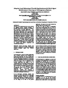
sive graph partitioners [22, 45, 58, 105] operate more locally than multilevel graph partitioners. Diffusive partitioners transfer work from heavily loaded processors to their more lightly loaded neighbors; “neighbors” are defined either by the network in the parallel computer or by a processor graph induced by the application’s data dependencies. Diffusive methods are faster than multilevel methods, but can require several iterations to achieve global balance. Diffusive partitioners are also more “incremental” than other graph partitioners; that is, small changes in processor work loads result in only small changes in the decomposition. This incrementality is important in dynamic load balancing, where the cost to move data to a new decomposition must be kept low. Graph partitioners allowing multiple weights per vertex (i.e., multiconstraint or multiphase partitioning) [54, 87, 102] or edge (i.e., multiobjective partitioning) [85] have been applied to a variety of multiphase simulations. Geometric partitioning methods can be effective alternatives to graph partitioners. Using only objects’ weights and physical coordinates, they assign equal object weight to processors while grouping physically close objects within subdomains. While they tend to produce partitions with higher communication costs than graph partitioning, they run faster and, in most cases, are implicitly incremental. Moreover, applications that lack natural graph connectivity (e.g., particle methods) can easily use geometric partitioners. Geometric recursive bisection uses a cutting plane to divide geometric space into two sets with equal object weight (Figure 1.1). The resulting subdomains are divided recursively in the same manner, until the number of subdomains equals the number of desired partitions. (This algorithm is easily extended from powers of two to arbitrary numbers of partitions.) Variants of geometric recursive bisection differ primarily in their choice of cutting plane. Recursive Coordinate Bisection (RCB) [6] chooses planes orthogonal to coordinate axes. Recursive Inertial Bisection (RIB) [91, 94] uses planes orthogonal to “long directions” in the geometry; these long directions are the principal axes of inertia. (Note that RIB is not incremental.) Unbalanced Recursive Bisection (URB) [48] generates subdomains with lower aspect ratio (and, by implication, lower communication costs) by dividing the geometry in half and then assigning a number of processors to each half that is proportional to the work in that half. Another geometric method, space-filling curve (SFC) partitioning, uses SFCs to map objects from their position in three-dimensional space to a linear ordering. Objects are assigned a “key” (typically an integer or a real number) representing the point on an SFC that is closest to the object. Sorting the keys creates the linear ordering of the objects. This linear ordering is then cut into equally weighted pieces to be assigned to partitions (Figure 1.2). SFC partitioners can be implemented in a number of ways. Different curves (e.g., Hilbert, Morton) may be used. The sorting step can be replaced by binning strategies [28]. An explicit octree representation of the SFC can be built [34, 63]. Topological connectivity can be used instead of coordinates to generate the SFC [65, 66]. In each approach, however, the speed of the algorithm and quality of the resulting decomposition is comparable to RCB.

i i

4

Chapter 1. Partitioning and Load Balancing (0,2) 1

3

1st cut: x=1.25 2nd cut

2nd cut

2nd cut: y=0.75

0

2nd cut: y=1.25

2

(0,0)

(3,0) 1st cut

0

1

2

3

Figure 1.1. Cutting planes (left) and associated cut tree (right) for geometric recursive bisection. Dots are objects to be balanced; cuts are shown with dark lines and tree nodes. 1

2

4. Second intersection

3. Start of 2nd search

2. First intersection 0

3

1. Start of 1st search

5. Start of 3rd search

Figure 1.2. SFC partitioning (left) and box-assignment search procedure (right). Objects (dots) are ordered along the SFC (dotted line). Partitions are indicated by shading. The box for box-assignment intersects partitions 0 and 2.

1.3

Beyond traditional applications

Traditional partitioners have been applied with great success to a variety of applications. Multilevel graph partitioning is highly effective for finite element and finite volume methods (where mesh nodes or cells are divided among processors). Diffusive graph partitioners and incremental geometric methods are widely used in dynamic computations such as adaptive finite element methods [6, 25, 32, 74, 84]. The physical locality of objects provided by geometric partitioners has been exploited in particle methods [80, 104]. Some new parallel applications can use enhancements of traditional partitioners with success. Contact detection for crash and impact simulations can use geometric and/or graph-based partitioners, as long as additional functionality for

i i

1.3. Beyond traditional applications

5

finding overlaps of the geometry with given regions of space is supported. Datamining applications often use graph partitioners to identify clusters within data sets; the partitioners’ objective functions are modified to obtain non-trivial clusters. Other applications, however, require new partitioning models. These applications are characterized by higher data connectivity and less homogeneity and symmetry. For example, circuit and density functional theory simulations can have much less data locality than finite element methods. Graph-based models do not sufficiently represent the data relationships in these applications. In this section, we describe some emerging parallel applications and appropriate partitioning solutions for them. We present techniques used for partitioning contact detection simulations. We survey application of graph-based partitioners to clustering algorithms for data mining. And we discuss hypergraph partitioning, an effective alternative to graph partitioning for less structured applications.

1.3.1

Partitioning for Parallel Contact/Impact Computations

A large class of scientific simulations, especially those performed in the context of computational structural mechanics, involve meshes that come in contact with each other. Examples include simulations of vehicle crashes, deformations, and projectile-target penetration. In these simulations, each iteration consists of two phases. During the first phase, traditional finite difference/element/volume methods compute forces on elements throughout the problem domain. In the second phase, a search determines which surface elements have come in contact with and/or penetrated other elements; the positions of the affected elements are corrected, elements are deformed, and the simulation progresses to the next iteration. The actual contact detection is usually performed in two steps. The first step, global search, identifies pairs of surface elements that are close enough to potentially be in contact with each other. In the second step, local search, the exact locations of the contacts (if any) between these candidate surfaces are computed. In global search, surface elements are usually represented by bounding boxes; two surface elements intersect only if their bounding boxes intersect. In parallel global search, surface elements first must be sent to processors owning elements with which they have potential interactions. Thus, computing the set of processors whose subdomains intersect a bounding box (sometimes called “box assignment”) is a key operation in parallel contact detection. Plimpton et al. developed a parallel contact detection algorithm that uses different decompositions for the computation of element forces (phase one) and the contact search (phase two) [80]. For phase one, they apply a traditional multilevel graph partitioner to all elements of the mesh. Recursive coordinate bisection (RCB) is used in phase two to evenly distribute only the surface elements. Between phases, data is mapped between the two decompositions, requiring communication; however, using two decompositions ensures that the overall computation is balanced and each phase is as efficient as possible. Because RCB uses geometric coordinates, potentially intersecting surfaces are likely to be assigned to the same processor, reducing communication during global search. Moreover, the box-assignment operation is very fast and efficient. The RCB decomposition is described fully by the

i i

6

Chapter 1. Partitioning and Load Balancing

tree of cutting planes used for partitioning (Figure 1.1). The planes are stored on each processor, and the tree of cuts is traversed to determine intersections of the bounding boxes with the processor subdomains. The use of a geometric method for the surface-element decomposition has been extended to space-filling curve (SFC) partitioners, due in part to their slightly faster decomposition times. Like RCB, SFC decompositions can be completely described by the cuts used to partition the linear ordering of objects. Box-assignment for SFC decompositions, however, is more difficult than for RCB, since SFC partitions are not regular rectangular regions. To overcome this difficulty, Heaphy et al. [28, 40] developed an algorithm based on techniques for database query [57, 67]. A search routine finds each point along the SFC at which the SFC enters the bounding box (Figure 1.2); binary searches through the cuts map each entry point to the processor owning the portion of the SFC containing the point. Multiconstraint partitioning can be used in contact detection. Each element is assigned two weights — one for force calculations (phase one) and a second for contact computations (phase two). A single decomposition that balances both weights is computed. This approach balances computation in both phases, while eliminating the communication between phases that is needed in the two-decomposition approach. However, solving the multiconstraint problem introduces new challenges. Multiconstraint or multiphase graph partitioners [54, 102] can be applied naturally to obtain a single decomposition that is balanced with respect to both the force and contact phases. These partitioners attempt to minimize interprocessor communication costs subject to the constraint that each component of the load is balanced. Difficulty arises, however, in the box-assignment operation, as the subdomains generated by graph partitioners do not have geometric regularity that can be exploited. One could represent processor subdomains by bounding boxes and compute intersections of the surface-element bounding box with the processor bounding boxes. However, because the processor bounding boxes are likely to overlap, many “false positives” can be generated by box assignment; that is, a particular surface element is said to intersect with a processor, even though none of the processor’s locally stored elements identify it as a candidate for local search. To address this problem, Karypis [50] constructs a detailed geometric map of the volume covered by elements assigned to each subdomain (Figure 1.3). He also modifies the multiconstraint graph decomposition so that each subdomain can be described by a small number of disjoint axis-aligned boxes; this improved geometric description reduces the number of false-positives. The boxes are assembled into a binary tree describing the entire geometry. Box assignment is then done by traversing the tree, as in RCB; however, the depth of the tree can be much greater than RCB’s tree. Boman et al. proposed a multicriteria geometric partitioning method that may be used for contact problems [12, 28]. Like the multiconstraint graph partitioners, this method computes one decomposition that is balanced with respect to multiple phases. Their algorithm, however, uses RCB, allowing box assignment to be done easily by traversing the tree of cuts (Figure 1.1). Instead of solving a multiconstraint problem, they solve a multiobjective problem: find as good a balance as possible with respect to all loads. While good multicriteria RCB decompositions do not always exist, heuristics are used to generate reasonable decompositions for many

i i

1.3. Beyond traditional applications

7 (J)

(I)

9 8

yes

(H)

Y−axis

6

y < 3.25

(D)

no

x < 5.00

7

5

y < 4.75

(F)

(E)

x < 6.00 y < 8.25

x < 7.00

(G) x < 2.50

(C)

4 3

y < 7.50

y < 6.25

2 1

(A)

(B) 1

2

3

4

5

6

7

8

9

X−axis (a) Partitioning of the contact points.

(b) Partitioning of the space.

(c) Associated Decision Tree

Figure 1.3. Use of multi-constraint graph partitioning for contact problems: (a) the 45 contact points are divided into three partitions; (b) the subdomains are represented geometrically as sets of axis-aligned rectangles; and (c) a decision tree describing the geometric representation is used for contact search. problems. In particular, they pursue the simpler objective X X min max(g( ai ), g( ai )), s

i≤s

i>s

where ai is the weight vector for object i, and g is a monotonically P non-decreasing function in each component of the input vector; typically g(x) = j xpj with p = 1 or p = 2, or g(x) = kxk for some norm. This objective function is unimodal with respect to s; that is, starting with s = 1 and increasing s, the objective decreases, until at some point the objective starts increasing. That point defines the optimal bisection value s, and it can be computed efficiently.

1.3.2

Clustering in Data Mining

Advances in information technology have greatly increased the amount of data generated, collected, and stored in various disciplines. The need to effectively and efficiently analyze these data repositories to transform raw data into information and, ultimately, knowledge motivated the rapid development of data mining. Data mining combines data analysis techniques from a wide spectrum of disciplines. Among the most extensively used data mining techniques is clustering, which tries to organize a large collection of data points into a relatively small number of meaningful, coherent groups. Clustering has been studied extensively; two recent surveys [39, 47] offer comprehensive summaries of different applications and algorithms. One class of clustering algorithms is directly related to graph partitioning; these algorithms model datasets with graphs and discover clusters by identifying well-connected subgraphs. Two major categories of graph models exist: similaritybased models [31] and object-attributed-based models [29, 109]. In a similarity-based graph, vertices represent data objects, and edges connect objects that are similar to each other. Edge weights are proportional to the amount of similarity between objects. Variations of this model include reducing the density of the graph by

i i

8

Chapter 1. Partitioning and Load Balancing

focusing on only a small number of nearest neighbors of each vertex, and using hypergraphs to allow set-wise similarity as opposed to pair-wise similarity. Objectattribute models represent how objects are related to the overall set of attributes. Relationships between objects and attributes are modeled by a bipartite graph G(Vo , Va , E), where Vo is the set of vertices representing objects, Va is the set of vertices representing attributes, and E is the set of edges connecting objects in Vo with their attributes in Va . This model is applicable when the number of attributes is very large, but each object has only a small subset of them. Graph-based clustering approaches can be classified into two categories: direct and partitioning-based. Direct approaches identify well-connected subgraphs by looking for connected components within the graph. Different definitions of the properties of connected components can be used. Some of the most widely used methods seek connected components that correspond to cliques and employ either exact or heuristic clique partitioning algorithms [23, 103]. However, this cliquebased formulation is overly restrictive and cannot find large clusters in sparse graph models. For this reason, much research has focused on finding components that contain vertices connected by multiple intra-cluster disjoint paths [5, 36, 38, 62, 88, 89, 93, 98, 108]. A drawback of these approaches is that they are computationally expensive, and, as such, can be applied only to relatively small datasets. Partitioning-based clustering methods use min-cut graph-partitioning algorithms to decompose the graphs into well-connected components [30, 51, 109]. By minimizing the total weight of graph edges cut by partition boundaries, they minimize the similarity between clusters, and, thus, tend to maximize the intra-cluster similarity. Using spectral and multilevel graph partitioners, high quality decompositions can be computed reasonably quickly, allowing these methods to scale to very large datasets. However, the traditional min-cut formulation can admit trivial solutions in which some (if not most) of the partitions contain a very small number of vertices. For this reason, most of the recent research has focused on extending the min-cut objective function so that it accounts for the size of the resulting partitions and, thus, produces solutions that are better balanced. Examples of effective objective functions are ratio cut (which scales the weight of cut edges by the number of vertices in each partition) [37], normalized cut (which scales the weight of cut edges by the number of edges in each partition) [90], and min-max cut (which scales the weight of cut edges by the weight of uncut edges in each partition) [30].

1.3.3

Partitioning for Circuits, Nanotechnology, Linear Programming and more

While graph partitioners have served well in mesh-based PDE simulations, new simulation areas such as electrical systems, computational biology, linear programming and nanotechnology show their limitations. Critical differences between these areas and mesh-based PDE simulations include high connectivity, heterogeneity in topology, and matrices that are structurally non-symmetric or rectangular. A comparison of a finite element matrix with matrices from circuit and density functional theory (DFT) simulations is shown in Figure 1.4; circuit and DFT matrices are more dense and less structured than finite element matrices. The structure of

i i

1.3. Beyond traditional applications

9

(a)

(b)

(c)

(d)

Figure 1.4. Comparing the non-zero structure of matrices from (a) a hexahedral finite element simulation, (b) a circuit simulation, (c) a density functional theory simulation, and (d) linear programming shows differences in structure between traditional and emerging applications.

linear programming matrices differs even more; indeed, these matrices are usually not square. In order to achieve good load balance and low communication in such applications, accurate models of work and dependency/communication are crucial. Graph models are often considered the most effective models for mesh-based PDE simulations. However, the edge-cut metric they use only approximates communication volume. For example, in Figure 1.5 (left), a grid is divided into two partitions (separated by a dashed line). Grid point A has four edges associated with it; each edge (drawn as an ellipse) connects A with a neighboring grid point. Two edges are cut by the partition boundary; however, the actual communication volume associated with sending A to the neighboring processor is only one grid point. Nonetheless, countless examples demonstrate graph partitioning’s success in mesh-based PDE applications where this approximation is often good enough. Another limitation of the graph model is the type of systems it can represent [41]. Because edges in the graph model are non-directional, they imply symmetry in all relationships, making them appropriate only for problems represented by square, structurally symmetric matrices. Structurally non-symmetric systems A must be represented by a symmetrized model, typically A + AT or AT A, adding new edges to the graph and further skewing the communication metric. While a

i i

10

Chapter 1. Partitioning and Load Balancing

A

A

Figure 1.5. Example of communication metrics in the graph (left) and hypergraph (right) models. Edges are shown with ellipses; the partition boundary is the dashed line.

directed graph model could be adopted, it would not improve the accuracy of the communication metric. Likewise, graph models cannot represent rectangular matrices, such as those arising in linear programming. Kolda and Hendrickson [42] propose using bipartite graphs. For an m×n matrix A, vertices ri , i = 1, . . . , m represent rows, and vertices cj , j = 1, . . . , n represent columns. Edges eij connecting ri and cj exist for non-zero matrix entries aij . But as in other graph models, the number of cut edges only approximates communication volume. Hypergraph models address many of the drawbacks of graph models. As in graph models, hypergraph vertices represent the work of a simulation. However, hypergraph edges (hyperedges) are sets of two or more related vertices. A hyperedge can thus represent dependencies between any set of vertices. The number of hyperedge cuts accurately represents communication volume [16, 18]. In the example in Figure 1.5 (right), a single hyperedge (drawn as a circle) including vertex A and its neighbors is associated with A; this single cut hyperedge accurately reflects the communication volume associated with A. Hypergraphs also serve as useful models for sparse matrix computations, as they accurately represent nonsymmetric and rectangular matrices. For example, the columns of a rectangular matrix could be represented by the vertices of a hypergraph. Each matrix row would be represented by a hyperedge connecting all vertices (columns) with non-zero entries in that row. A hypergraph partitioner, then, would assign columns to processors while attempting to minimize communication along rows. One could alternatively let vertices represent rows and edges represent columns to obtain a row-partitioning. Optimal hypergraph partitioning, like graph partitioning, is NP-hard, but good heuristic algorithms have been developed. The dominant algorithms are extensions of the multilevel algorithms for graph partitioning. Hypergraph partitioning’s effectiveness has been demonstrated in many areas, including VLSI layout [14], sparse matrix decompositions [18, 99], and database storage and data mining [21, 73]. Several (serial) hypergraph partitioners are available (e.g., hMETIS [52], Pa-

i i

1.4. Beyond traditional approaches

11

ToH [18, 17], MLPart [15], Mondriaan [99]), and two parallel hypergraph partitioners for large-scale problems are under development: Parkway [97], which targets information retrieval and Markov models, and Zoltan-PHG [27], part of the Zoltan [11] toolkit for parallel load balancing and data management in scientific computing.

1.4

Beyond traditional approaches

While much partitioning research has focused on the needs of new applications, older, important applications have not been forgotten. Sparse matrix-vector multiplication, for example, is a key component of countless numerical algorithms; improvements in partitioning strategies for this operation can greatly impact scientific computing. Similarly, because of the broad use of graph partitioners, algorithms that compute better graph decompositions can influence a range of applications. In this section, we discuss a few new approaches to these traditional problems.

1.4.1

Partitioning for sparse matrix-vector multiplication

A common kernel in many numerical algorithms is multiplication of a sparse matrix by a vector. For example, this operation is the most computationally expensive part of iterative methods for linear systems and eigensystems. More generally, many data dependencies in scientific computation can be modeled as hypergraphs, which again can be represented as (usually sparse) matrices (see §1.3.3). The question is how to distribute the nonzero matrix entries (and the vector elements) in a way that minimizes communication cost while maintaining load balance. The sparse case is much more complicated than the dense case, and is a rich source of combinatorial problems. This problem has been studied in detail in [17, 18] and in [10, Ch.4]. The standard algorithm for computing u = Av on a parallel computer has four steps. First, we communicate entries of v to P processors that need them. Second, we compute local contributions of the type j aij vj for certain i, j and store them in u. Third, we communicate entries of u. Fourth, we add up partial sums in u. The simplest matrix distribution is a one-dimensional (1D) decomposition of either matrix rows or columns. The communication needed for matrix-vector multiplication with 1D distributions is demonstrated in Figure 1.6. C ¸ ataly¨ urek and Aykanat [17, 18] realized that this problem can be modeled as a hypergraph partitioning problem, where, for a row distribution, matrix rows correspond to vertices and matrix columns correspond to hyperedges, and vice versa for a column distribution. The communication volume is then exactly proportional to the number of cut hyperedges in the bisection case; if there are more than two partitions, the number of partitions covering each hyperedge has to be taken into account. The 1D hypergraph model reduced communication volume by 30–40% on average versus the graph model for a set of sparse matrices [17, 18]. Two-dimensional (2D) data distributions (i.e., block distributions) are often better than 1D distributions. Most 2D distributions used are Cartesian; that is, the matrix is partitioned both along rows and columns in a grid-like fashion and each processor is assigned the nonzeros within a rectangular block. The Cartesian 2D

i i

12

Chapter 1. Partitioning and Load Balancing 2

6 9

1

4

3

1

1

V

2

6 9

5

9

6

64 U

4

3

22 41

1

5 A

2 3

41

8

9

64 U

1

4

4

3

V

1

3

22

5

1

1 9

5 6

5

2 5

3

8

9

A

Figure 1.6. Row (left) and column (right) distribution of a sparse matrix for multiplication u = Av. There are only two processors, indicated by dark and light shading, and communication between them is shown with arrows. In this example, the communication volume is three words in both cases. (Adapted from [10, Ch.4].)

distribution is inflexible and good load balance is often difficult to achieve, so variations like jagged or semi-general block partitioning have been proposed [61, 77, 83]. These schemes first partition a matrix into p1 strips in one direction, and then partition each strip independently in the orthogonal direction into p2 domains, where p1 × p2 is the total number of desired partitions. Vastenhow and Bisseling have recently suggested a non-Cartesian distribution called Mondriaan [99]. The method is based on recursive bisection of the matrix into rectangular blocks, but permutations are allowed and the cut directions may vary. Each bisection step is solved using hypergraph partitioning. Mondriaan distributions often have significantly lower communication costs than 1D or 2D Cartesian distributions [99]. In the most general distribution, each nonzero (i, j) is assigned to a processor with no constraints on the shape or connectivity of a partition. (See Figure 1.7 for an example.) C ¸ ataly¨ urek and Aykanat [16, 19] showed that computing such general (or fine-grain) distributions with low communication cost can also be modeled as a hypergraph partitioning problem, but using a different (larger) hypergraph. In their fine-grain model, each nonzero entry corresponds to a vertex and each row or column corresponds to a hyperedge. This model accurately reflects communication volume. Empirical results indicate that partitioning based on the fine-grain model has communication volume that is lower than 2D Cartesian distributions [19]. The disadvantage of using such complex data distributions is that the application needs to support arbitrary distributions, which is typically not the case. After a good distribution of the sparse matrix A has been found, vectors u and v still must be distributed. In the square case, it is often convenient to use the same distribution, but it is not necessary. In the rectangular case, the vector distributions will obviously differ. Bisseling and Meesen [10, 9] have studied this

i i

1.4. Beyond traditional approaches 2

6 9

1

1

4

3

V

1

1 9

5 6

5

64 U

4

3

22 41

13

2 5

3

8

9

A

Figure 1.7. Irregular matrix distribution with two processors. Communication between the two processors (shaded dark and light) is indicated with arrows.

vector partitioning problem, and suggest that the objective for this phase should be to balance the communication between processors. Note that a good matrix (hypergraph) partitioning already ensures that the total communication volume is small. For computing u = Av, no extra communication is incurred as long as vj is assigned to a processor that also owns an entry in column j of A, and ui is assigned to a processor that contains a nonzero in row i. There are many such assignments; for example, in Figure 1.7, u3 , u4 , and v5 can all be assigned to either processor. The vector partitions resulting from different choices for these particular vector entries are all equally good measured by total communication volume. One therefore has flexibility (see also Section 1.5.2 on flexibly assignable work) to choose a vector partitioning that minimizes a secondary objective, such as the largest number of send and receive operations on any processor. (Similar objectives are used in some parallel cost models, like the BSP model [10].) Bisseling and Meesen [10, 9] have proposed a fast heuristic for this problem, a greedy algorithm based on local bounds for the maximum communication for each processor. It is optimal in the special case where each matrix column is shared among at most two processors. Their approach does not attempt to load balance the entries in u and v between processors because doing so is not important for matrix-vector multiplication.

1.4.2

Semidefinite programming for graph partitioning

Although multilevel algorithms have proven quite efficient for graph partitioning, there is ongoing research into algorithms that may give higher quality solutions (but may also take more computing time). One such algorithm uses semidefinite programming (SDP). The graph partitioning problem can be cast as an integer programming problem. Consider the bisection problem where the vertices of a graph G = (V, E) shall

i i

14

Chapter 1. Partitioning and Load Balancing

be partitioned into two approximately equal sets P0 and P1 . Let x ∈ {−1, 1}n be an assignment vector such that xi = −1 if vertex vi ∈ P0 and xi = 1 if it is in P1 . It is easy to see that the number of edges crossing from P0 to P1 is 1 4

X

(xi − xj )2 =

(i,j)∈E,i