Apply fixed point theorem for solving of nonlinear Volterra integral equation with Harr wavelet Majid. Erfanian, Morteza. Gachpazan Department of Science, School of Applied Mathematics, University of Zabol
[email protected]. Department of Applied Mathematics, School of Mathematical Sciences, Ferdowsi University of Mashhad,
[email protected]
abstract In this article, we present a method for numerical approximation of fixed point operator, particularly for the integral one associated to a nonlinear Volterra integral equation, which uses the properties of rationalized Haar wavelets. The main tools for error analysis is Banach fixed point theorem. Furthermore, the order of convergence is analyzed. Some numerical examples are included to support the theory.
keywords NonlinearVolterra integral equation; Rationalized Haar wavelet; Operational matrix; fixed point theorem. MSC 2010: 47A56; 45B05; 47H10; 42C40.
1- Introduction and preliminaries Analytical solutions of integral equations, either do not exist or are hard to find. Due to this, many numerical methods have been developed for finding the solutions of integral equations. The use of wavelets has come to prominence during the last two decades. Various types of wavelets have been applied for numerical solution of different kinds of integral equations. These include Haar, Legendre, trigonometric, CAS, Chebyshev, and Coifman wavelets. Lepik and Tamme in [1] have applied Haar wavelets to solve nonlinear Fredholm integral equations, but their method involves approximation of certain integrals. The orthogonal
set of Haar functions is a group of square waves with magnitude of 2" , $2" and 0, for any i % 0,1, …. The aim of this work is to present a numerical method to approximating the solution of nonlinear Volterra integral equations of the second kind as follows: !
1.1
u&x' % f&x'
α )- *&x, t', u&t''dt ,
1.2
BD.&='E % F&='
+
!
. ∈ 3 % 4&50,16'.
where f: 50, 16 → R, α ∈ R, and W: 50,16 9 R → R is a continuous function such that there exist ; < 0 where satisfy a global Lipschitz condition for = ∈ 50,16 and for all >, ? ∈ @, namely |*&=, >' $ *&=, ?'| A ;|> $ ?|. The integral operator B: &3, ||. ||C ' → &3, ||. ||C ' is also defined as
2- Numerical approximation of the solution
G )- *&x, t', u&t''HI , I ∈ 50, 16. J
Definition 2.1 The RH wavelet is the function defined on the real line @ as follows: 1
K&I' % L$1 0
N O
0M IA
M I M 1,
PIQSTUVXS.
N O
,
The RH functions QY &I', for any Z % 1,2, … where [ % 2\ ], with V % 0,1, … and ] % 0,1, … , 2\ $ 1, are defined by QY &I' % K&2\ I $ ]'|5-,N6. For any =, I ∈ 50, 16, and Z ^ 1 and _ % 2`aN ∈ b, we define .` &=' % F&='
2.1 That if we set:
α )- *&=, I, .`cN 'HI , J
e`cN &=, I': % *&=, I, .`cN &I''.
2.2
Z % 1,2, . . ..
If gh be an orthogonal projection with following interpolation property we have
Or in the matrix form 2.3
hcN gh &e'&=, I' % ∑hcN \l- ∑kl- X\k Q\ &='Qk &I'. &O'
gh &e'&=, I' % mn &='om&I'.
That vector m is defined by m % 5Q- &=', QN &=', . . . , QhcN &='6n .Also we have: )- m&X' HX % pm&=', J
2.4
where p is a _ 9 _ operational matrix for integration and is defined by ph9 h
h 9 1 2_ph % q cN O O s h h 2_ r 9 O
O
sh h $r 9 O
0
O
v,
s h9h is r s h9h % ym z { , m z { , … , m& wherein rN9N % 516, wN9N % 5O6, and r Oh Oh N
s cN h9h % r
N
h
N
}
OhcN Oh
'~, while
h h } s n h9h . €•‚ƒ „1,1,2,2, †‡ r 2O‡ˆ‡ , . . . ‡‰ , 2O , 2 , . . . , Œ. , . . . ‡‰ , 2} , … , †‡ˆ‡‰ †‡ ‡ˆ‡ O"
OŠ
O
‹ "
O
Note that wherein o % •XYŽ • , for • % 1,2 and XYŽ % 2 " 〈QY &=', 〈e&=, I', QŽ &I'〉〉 , h9 h ‘’“
with V, ] % 0,1, . . . , where [ % 2k
•, • % 0,1, . . . , 2k $ 1, and – % 2\
2.5
™ cN s s cN s h9 ˜ % Dr h E . o. DšEh9 h ,
Thus by using this equation we have
• — , • — % 0,1, . . . , 2\ $ 1,
s % 5X̂\k 6h9 h , and V, ] % 1,2, . . . , _ as X̂\k % e z where o
O\cN OkcN , { Oh Oh
V, ] % 1,2, . . . , _.
Thus for the Volterra integral equations we have: 2.6
.` &=' % F&='
α )- gh &e`cN '&=, I'HI ,
Z % 1,2, . . ..
J
3- Error analysis In this section, by using the Banach fixed point theorem, we get an upper bound for the error of the our method, and the order of convergence is analyzed.
Lemma 3-1. Let *: 50,16O 9 œ → œ, be continiouse and Lipschitzian with Lipschitz constant ; , then B has an unique fixed point and for all .- ∈ 4&50,16' where – % |G|; M 1, and . is the fixed point of B. 3.1
k •. $ B \ &.- '•C A ‖B&.- ' $ .- ‖C 9 ∑C kl\ – ,
Theorem 3.1. Assume that e\cN ∈ 4&50,16O ', and Ÿ.\ \¡ Nis a subset of 4&50,16', and * ∈ 4&50,16O 9 œ', are lipschitzian functions at its third variable, if ¢ is a constant then we have 3.2
4- Numerical examples
k ‖. $ .\ ‖C A ‖B&.- ' $ .- ‖C ∑C kl\ –
¢.
In this section by using the method presented in (3.12, 3.13) are solved some examples from different references. The main characteristic of this technique is that does not lead to a nonlinear algebraic equations system. The following algorithm, based on the method presented in Section 3, has been used to solve Examples 1 to 3. Algorithm 4.1
1. Produce matrices m&I', £h9 h , ¤ZH p. 2. For V % 1to • do, s 3. Product Matrix o, o 4. Compute gh &e'&=, I' from 3.3 or 3.4. 5. Compute .\ &I' from 3.12 or 3.12 for the assumed point. 6. Go to step 2. Example 4.1. Let us consider the nonlinear Volterra Hammerstein integral equation of the second kind 4.1 where
.&I' % F&I'
)-
¦ ¥Š ¦ " O
¤T¢I¤ZD.&X'EHX,
F&I' % I $ I O & I ¨ ¤T¢I¤Z&I' $ N §
N
O¨
I}
N §
I $ ¤T¢I¤Z&I'', N §
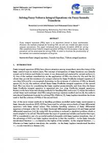
and .&0' % 0, and the exact solution is .&I' % I. The comparison between the approximated solutions obtained by the Haar wavelet method, collocationtype method [2] and Legendre wavelets method [3] is given in Table 4. We see that there is a good
agreement of results between these three methods. This fact justifies the ability, efficiency and applicability of the present method. In Fig. 3, comparison between analytical and approximated solutions is shown. The run time for _ % 128 is about 11.797 seconds. I\
0.12109375 0.24609375 0.37109375 0.49609375 0.62109375 0.74609375 0.87109375 0.99609375
Table 1. Numerical results for Example 4.1
collocation-type method[2] With ¬ % 65 1.68 9 10c° 1.44 9 10c´ 1.78 9 10c´ 1.02 9 10c¨ 3.90 9 10c¨ 1.14 9 10c} 2.81 9 10c} 6.07 9 10c}
Legendre wavelets method[3] With • % 1, ; % 6 6.90 9 10c± 5.36 9 10c¯ 6.39 9 10c° 3.61 9 10c´ 1.35 9 10c´ 3.96 9 10c° 9.67 9 10c° 2.07 9 10c´
Presented method With _ % 2¯ 3.10 9 10cN9.01 9 10c± 6.72 9 10c§ 2.75 9 10c¯ 8.14 9 10c¯ 1.98 9 10c° 4.31 9 10c° 8.829 10c°
Figure 1: Comparison of exact and approximate solutions for Example 4.1
References [1] K. E. Atkinson: The Numerical Solution of Integral Equations of the Second Kind, Cambridge University Press, 1997. [2] K. Kumar and I. H. Sloan: A new collocation-type method for Hammerstein integral equations, Math. Comp.48(1987), no. 178, 585-593. [3] S. Yousefi, M. Razzaghi: Legendre wavelets method for the nonlinear VolterraFredholm integral equations, Mathematics and Computers in Simulation 70 (2005) 18.