Numerical Method for solving Volterra Integral

IAENG International Journal of Applied Mathematics, 43:4, IJAM_43_4_03 ______________________________________________________________________________________

Numerical Method for solving Volterra Integral Equations with a Convolution Kernel Changqing Yang, Jianhua Hou

Abstract—This paper presents a numerical method for solving the Volterra integral equation with a convolution kernel. The integral equation was first converted to an algebraic equation using the Laplace transform, after which its numerical inversion was determined by power series. The Padé approximants were effectively used to improve the convergence rate and accuracy of the computed series. The method is described and illustrated with numerical examples. The results revealed that the method is accurate and easy to implement.

main advantage of this method is its simplicity, such that only few of the terms of the expansion are needed to obtain good convergent numerical results.

Index Terms—Volterra integral equation, Laplace transform, Taylor expansion, series solution, Padé approximant.

Definition II.1. The Laplace transform of a function f (x), x > 0 is defined as Z +∞ L[f (x)] = F (s) = e−sx f (x)dx,

I. I NTRODUCTION

V

OLTERRA integral equations have many applications in various areas, including mathematical physics, chemistry, electrochemistry, semi-conductors, scattering theory, seismology, heat conduction, metallurgy, fluid flow, chemical reaction and population dynamics[1], [2]. This paper focuses on a class of Volterra integral equations with a convolution kernel given by Z x u(x) = f (x) + k(x − t)u(t)dt, x ∈ [0, T ], (1) 0

where the source function f and the kernel function k are given, and u(x) is the unknown function. Several numerical methods are available for approximating the Volterra integral equation. In particular, Huang[3] used the Taylor expansion of unknown function and obtained an approximate solution. Yang[4] proposed a method for the solution of integral equation using the Chebyshev polynomials, while Yousefi[5] presented a numerical method for the Abel integral equation by Legendre wavelets. Khodabin [6] numerically solved the stochastic Volterra integral equations using triangular functions and their operational matrix of integration. Kamyad [7] proposed a new algorithm based on the calculus of variations and discretisation method, in order to solve linear and nonlinear Volterra integral equations. The Adomian decomposition [8], [9], [10], Homotopy perturbation [10], [11] and the Laplace decomposition methods[12] were proposed for obtaining the approximate analytic solution of the integral equation. In this paper, Volterra integral equations were first reduced to algebraic equations using the Laplace transform. We obtained a series that was uniformly convergent to the exact solution after applying the Taylor expansion and the inverse Laplace transforms to the mentioned algebraic equations. The Manuscript received May 13, 2013; revised July 02, 2013. This work was supported by Huaihai institute of technology under Grant Z2012021 C. Yang is with the Department of Science, Huaihai Institute of Technology, Lianyungang, Jiangsu, 222005 China e-mail: ([email protected]). H. Hou is with the Department of Science, Huaihai Institute of Technology, Lianyungang, Jiangsu, 222005 China e-mail: ([email protected]).

II. L APLACE TRANSFORM AND THEIR PROPERTIES This section provides the definition and properties of the Laplace transform[13].

0

where s can either be real or complex. The Laplace transform has several properties, as explained below: 1) Linearity property L[af (x) + bg(x)] = aL[f (x)] + bL[g(x)], where a, b are constants. 2) The convolution theorem Let the Laplace transforms for the functions f1 (x) and f2 (x) be given by L[f1 (x)] = F1 (s), L[f2 (x)] = F2 (s). The Laplace convolution product of these two functions is defined by ·Z x ¸ L f1 (x − t)f2 (t)dt = F1 (s)F2 (s), (2) 0

Theorem II.2. [13] Suppose F (s) is the Laplace transform of f (x), which has a Maclaurin power series expansion in the form ∞ X xi (3) f (x) = ai . i! i=0 Taking the Laplace transform, it is possible to write formally F (s) =

∞ X ai . i+1 s i=0

(4)

Conversely, we derive (3) form a given expansion (4). III. PAD E´ APPROXIMANT A Padé approximant refer to the ratio of two polynomials constructed from the coefficients of the Taylor series expansion of a function. The [L/M ] Padé approximant to a formal P∞ power series y(t) = i=0 ai ti is given by: · ¸ PL (t) p0 + p1 t + · · · + pL tL L = = . (5) M QM (t) 1 + q1 t + · · · + qM tM

(Advance online publication: 29 November 2013)

IAENG International Journal of Applied Mathematics, 43:4, IJAM_43_4_03 ______________________________________________________________________________________ The two polynomials in the numerator and denominator of (5) have no common factor, thus indicating the formal power series expressed by y(t) =

PL (t) + O(tL+M +1 ). QM (t)

V. N UMERICAL EXAMPLES In this section, the effectiveness and simplicity of the proposed method were demonstrated using three examples. All the results were calculated using the symbolic calculus software Mathematica.

In this case, the Padé approximant [L/M ] is uniquely determined.

Example V.1. Consider the Abel integral equation given by Z x u(t) √ dt = e−x − 1, x ∈ [0, 1]. (7) x−t 0

IV. S OLUTION OF VOLTERRA INTEGRAL EQUATION AND

We using the Laplace transform and convolution property given by 1 L[u]L[x− 2 ] = L[e−x − 1],

ERROR ESTIMATE

In this section we solved Volterra integral equation (1) by the Laplace transform and Taylor series. First, the Laplace transform is applied to both sides of Equation(1) ·Z

¸

x

L[u(x)] = L[f (x)] + L

k(x − t)u(t)dt 0

Using the Laplace transform property (2), the equation below can be obtained L[u] = L[f ] + L[k]L[u]. Thus, the given equation is equivalent to L[u] =

L[f ] = F (s). 1 − L[k]

Applying Theorem(II.2), F (s) can be expanded as an absolutely convergent series, which is given by L[u] =

c2 c3 c1 + 2 + 3 + ··· s s s

where c1 , c2 , c3 , · · · are the known constants. Considering the inverse Laplace transform on both sides of the above equation, we can then obtain u(x) = c1 +

c3 2 c4 3 c2 x+ x + x ··· Γ (2) Γ (3) Γ (4)

(6)

which is uniformly convergent to the exact solution. We approximate the solution u(x) by using c3 2 c2 cn n−1 x+ x + ··· + x . un (x) = c1 + Γ (2) Γ (3) Γ (n) Let en (x) = u(x)−un (x) be the error function, where un (x) is the estimation of the true solution u(x). Using Taylor’s theorem and assuming that |u(n) (x)| ≤ M , the equation below can be obtained |en | = |u(x) − un (x)| ≤ M

cn+1 |xn |. Γ (n + 1)

Padé approximants have the advantage of manipulating the polynomial approximation into a rational function in order to gain more information about u(x). Consequently, the series (6) should be manipulated to construct Padé approximants, such that the performance of the approximants shows superiority over the series solutions.

so that

−1 = F (s). L[u] = √ √ π s(s + 1)

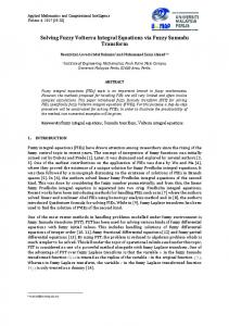
Expanding the right hand side F (s) in the power of 1/s, we obtain Ã µ ¶3 µ ¶5 µ ¶7 µ ¶9 ! 1 2 1 2 1 2 1 2 1 − + − + ··· . L[u] = √ s s s s π By taking the inverse Laplace transform of both sides of the above equation, the series solution can new be expressed as: √ µ 2 4 8 3 −2 x 1 − x + x2 − x u(x) = π 3 15 105 32 5 64 16 4 (8) x − x + x6 + 945 10395 135135 ¶ 256 128 x7 − x8 · · · , − 2027025 34459425 which is consistent with the results obtained in a previous work[9]. Padé approximants also have the advantage of manipulating the polynomial approximation into a rational function to gain more information about u(x). The Padé approximants [3/3], [4/4] and [5/5] of u(x) were constructed in order to study the structure of the obtained solution(8). For example, the Padé approximants [4/4] is given by √ 10 88 2048 x + x2 − 23205 x3 + 11486475 x4 −2 x 1 − 51 . · u(x) ≈ 8 2 32 16 8 π x + 85 x + 3315 x3 + 36465 x4 1 + 17 The numerical results show in Fig.1. Example V.2. Consider the Abel integral equation of second kind expressed as[5], [14]: Z x √ u(t) √ dt, x ∈ [0, 1]. (9) u(x) = 2 x − x−t 0 √ πx The exact √ solution is u(x) = 1 − e erf c( πx), where erf c( πx) is the complementary error function and defined as Z ∞ 2 2 √ e−t dt. erf c(x) = π x Applying the Laplace transform and convolution property (2), we arrive at √ 1 L[u] = L[2 x] − L[x− 2 ]L[u]. Hence, L[u] =

√ L[2 x] 1

1 + L[x− 2 ]


,


−0.325

0.8 [3/3] [4/4] [5/5]

Approximate solution exact solution

0.7

−0.33 0.6 0.5 u(x)

u(x)

−0.335

−0.34

0.4 0.3 0.2

−0.345 0.1 −0.35 0.5

0.6

0.7

0.8

0.9

0 0

1

0.2

0.4

x

Fig. 1.

0.6

0.8

1

x

Fig. 2.

Numerical results for Example1

Comparison of approximate solutions [4/4] and exact solution TABLE I C OMPUTED ABSOLUTE ERRORS FOR E XAMPLE V.2

or equivalently, L[u] =

√ π √ = F (s). s( s + π)

x

The right hand side of F (s) expanded in the power of 1/s as in µ ¶ 23 µ ¶ 25 µ ¶2 3 1 1 1 1 + π2 −π F (s) =π 2 s s s µ ¶ 27 µ ¶4 µ ¶3 5 1 1 1 2 2 2 (10) +π −π −π s s s µ ¶ 29 µ ¶5 7 1 1 ··· . − π4 + π2 s s

Presented method [3/3]

Presented method [3/3]

Wavelets method (k = 0, M = 16)

0

0

0

0

0.1

7.26464 × 10−7

4.33846 × 10−9

1.15872 × 10−2

0.2

4.50941 × 10−6

4.87786 × 10−8

1.13995 × 10−2

0.3

1.21047 ×

10−5

1.82276 ×

10−7

9.55367 × 10−3

2.34327 ×

10−5

4.42272 ×

10−7

1.68378 × 10−3

3.81788 ×

10−5

8.53771 ×

10−7

7.61903 × 10−3

5.59739 ×

10−5

1.43214 ×

10−6

1.53846 × 10−3

7.64562 ×

10−5

2.18575 ×

10−6

3.09894 × 10−3

9.92936 ×

10−5

3.11805 ×

10−6

2.98197 × 10−3

1.24188 ×

10−4

4.22898 ×

10−6

7.08482 × 10−4

0.4 0.5 0.6 0.7 0.8 0.9

By applying the inverse Laplace transform to (10), we obtain π 2 2 5π 2 5 4π 3 x2 − x + x2 3 2 18 π4 4 π 3 3 16π 3 5 x + x2 − x ··· . − 6 105 24 1

u(x) =2x 2 − πx +

(11)

1

Similarly, t = x 2 was first substituted, the Padé approximant [3/3] and [4/4] of u(t) was constructed, and the approximation [4/4] was provided to the solution: 1

u(x) ≈

√ √ x The exact solution is u(x) = 2 3 3 sin( 3x/2)e− 2 . Taking the Laplace transforms of both sides of (12) can yield ·Z x ¸ L[u] + L cos(x − t)u(t)dt = L[sin(x)] 0

Applying (2) we obtain L[u] + L [cos(x)] L[u] = L[sin(x)],

3

2x 2 + 3.0829x + 2.0808x 2 + 0.5207x2 1 2

3 2

.

1 + 3.1123x + 3.8347x + 2.2230x + 0.5235x2 The results shown in Fig. 2 demonstrate that the approximate solutions obtained using the proposed method are in good agreement with the exact solutions. When the solution u(x) has a special form, the proposed method works well. Furthermore, the numerical results in Table1 reveal that higher order accuracy can be achieved by increasing some terms of the expansion. In this way, more terms would enhance the level of accuracy of the numerical approximation. Moreover, by comparing the results of the table, the results of the presented method are more accurate than those of the wavelet method presented in a previous work[14]. Example V.3. Consider the Volterra integral with a convolution kernel given by[15] Z x u(x) + cos(x − t)u(t)dt = sin(x). (12) 0

which provides L[u] =

1 L[sin(x)] . = 2 1 + L[cos(x)] s +s+1

Expanding the right hand side of the above equation in power of 1/s, we obtain L[u] =

1 1 1 1 1 1 1 1 − 3 + 5 − 6 + 8 − 9 + 11 − 12 · · · . 2 s s s s s s s s

Applying the inverse Laplace transform to the above equation, we obtain u(x) = x −

x4 x5 x7 x8 x10 x11 x2 + − + − + − ··· . 2 4! 5! 7! 8! 10! 11!

We construct the Padé approximants [3/3], [4/4] and [5/5]


IAENG International Journal of Applied Mathematics, 43:4, IJAM_43_4_03 ______________________________________________________________________________________ TABLE II A BSOLUTE ERRORS OF [3/3], [4/4] AND [5/5] FOR E XAMPLE V.3 x

[3/3]

[4/4]

0

0

0

0

0.1

2.47996 × 10−13

2.12330 × 10−15

4.16334 × 10−17

0.2

6.34643 × 10−11

1.04025 × 10−12

3.05311 × 10−16

0.3

1.62565 ×

10−9

3.81095 ×

10−11

2.86993 × 10−14

1.62261 ×

10−8

4.83148 ×

10−10

6.49258 × 10−13

9.66243 ×

10−8

3.42285 ×

10−9

7.20879 × 10−12

4.14996 ×

10−7

1.67752 ×

10−8

5.10483 × 10−11

1.42247 ×

10−6

6.37358 ×

10−8

2.64983 × 10−10

4.13357 ×

10−6

2.00938 ×

10−7

1.09561 × 10−9

1.05880 ×

10−5

5.49231 ×

10−7

3.80688 × 10−9

2.45509 ×

10−5

1.34114 ×

10−6

1.15307 × 10−8

0.4 0.5 0.6 0.7 0.8 0.9 1

[5/5]

of u(x): 3 · ¸ x + x2 − 9x 3 20 , = 3x2 13x3 3 1 + 3x 2 + 10 + 120 2 · ¸ 113x3 149x4 x − 48x 4 223 − 1561 + 9366 , = 437x2 173x3 470x4 4 1 + 127x 446 + 6244 + 18732 + 374640 2 · ¸ 775x3 1285x4 49363x5 x − 4205x 5 12627 − 16836 + 50508 − 21213360 . = 473x2 11x3 1277x4 797x5 5 1 + 4217x 25254 + 12627 + 4392 + 4242672 − 42426720

[6] M. Khodabin, K. Maleknejad, and F. H. Shekarabi, “Application of triangular functions to numerical solution of stochastic Volterra integral equations,” IAENG International Journal of Applied Mathematics, vol. 43, no. 1, pp. 1–9, 2013. [7] A. V. Kamyad, M. Mehrabinezhad, and J. Saberi-Nadjafi, “A numerical approach for solving linear and nonlinear Volterra integral equations with controlled error,” IAENG International Journal of Applied Mathematics, vol. 40, no. 2, pp. 27–32, 2010. [8] G. Adomian, Frontier Problem of Physics: The Decomposition Method. Kluwer Academic Publish, 1994. [9] L. Bougoffa, R. C. Rach, and A. Mennouni, “A convenient technique for solving linear and nonlinear Abel integral equations by the Adomian decomposition method,” Applied Mathematics and Computation, vol. 218, no. 5, pp. 1785–1793, 2011. [10] R. K. Pandey, O. P. Singh, and V. K. Singh, “Efficient algorithms to solve singular integral equations of Abel type,” Computers & Mathematics with Applications, vol. 57, no. 4, pp. 664–676, 2009. [11] J. H. He, “Homotopy perturbation technique,” Computer Methods in Applied Mechanics and Engineering, vol. 178, no. 3-4, pp. 257–262, 1999. [12] M. Khan and M. A. Gondal, “A reliable treatment of Abel’s second kind singular integral equations,” Applied Mathematics Letters, vol. 25, no. 11, pp. 1666–1670, 2012. [13] L. Debnath and D. Bhatta, Integral Transforms and their Applications, 2nd ed. Chapmanand & Hall/CRC Press, 2007. [14] S. Sohrabi, “Comparison Chebyshev wavelets method with BPFs method for solving Abel’s integral equation,” Ain Shams Engineering Journal, vol. 2, no. 3-4, pp. 249–254, 2011. [15] S. A. Isaacsona and R. M. Kirby, “Numerical solution of linear Volterra integral equations of the second kind with sharp gradients,” Journal of Computational and Applied Mathematics, vol. 235, no. 1415, pp. 4283–4301, 2011.

The numerical results shown in Fig. 3 and Table 2 reveal that higher order accuracy can be achieved by increasing some terms of the expansion, that is, using more terms can enhance the level of accuracy of the numerical approximation. This fact ensures that the method is convergent. VI. C ONCLUSION In this paper, we applied Laplace transform and Taylor series to solve the Volterra integral equation with a convolution kernel. The properties of the Laplace transform, together with Taylor series, are used to reduce the integral equations to the algebraic equations. The method requires much less computational work compared with traditional methods. Although we only considered a model problem in this paper, the main ideas and techniques used here are also applicable to many other problems.

Changqing Yang He was born in Shanxi, China, in 1973. He received the bachelor and master degrees in mathematics from Chengdu University of Technology in 1997 and 2004, respectively. His main research interests are in numerical methods on integral equations and spectral method.

ACKNOWLEDGMENT The authors are grateful to anonymous reviewers for their valuable comments. R EFERENCES [1] H. J. Teriele, “Collocation method for weakly singular second kind Volterra integral equations with non-smooth solution,” IMA Journal of Numerical Analysis, vol. 2, no. 4, pp. 437–449, 1982. [2] P. K. Lamm and L. Eldén, “Numerical solution of first-kind Volterra equations by sequential Tikhonov regularization,” SIAM Journal on Numerical Analysis, vol. 34, no. 4, pp. 1432–1450, 1997. [3] L. Huang, Y. Huang, and X. Li, “Approximate solution of Abel integral equation,” Computers & Mathematics with Applications, vol. 56, no. 7, pp. 1748–1757, 2008. [4] C. Yang, “Chebyshev polynomial solution of nonlinear integral equations,” Journal of the Franklin Institute, vol. 349, no. 3, pp. 947–956, 2012. [5] S. A. Yousefi, “Numerical solution of Abel’s integral equation by using Legendre wavelets,” Applied Mathematics and Computation, vol. 175, no. 1, pp. 574–580, 2006.

Jianhua Hou She was born in Shanxi, China, in 1978. She received her bachelor in computer science in 1998 from the Shanxi Normal University. Her master degree was obtained in 2004 from the Chengdu University of Technology, Sichuan, China. Her main research interests are in parallel numerical algorithms.



0.6

exact solution [3/3] [4/4] [5/5]

0.5

0.4

u(x)

0.3

0.2

0.1

0

−0.1 0

Fig. 3.

0.5

1

1.5 x

2

2.5

Comparison of approximate solutions [3/3],[4/4],[5/5] and exact solution


3