Applying Alternative Variance Estimation Methods for Totals Under ...

Section on Survey Research Methods – JSM 2010

Applying Alternative Variance Estimation Methods for Totals Under Raking in SOI’s Corporate Sample Kimberly Henry1, Valerie Testa1, and Richard Valliant2 Statistics of Income, P.O. Box 2608, Washington DC 20013-2608 2 University of Michigan, 1218 Lefrak Hall, College Park MD 20742 1

Abstract: SOI’s Tax Year 2006 Corporate sample is a stratified Bernoulli sample of approximately 110,000 corporate income tax returns. Raking adjustments are performed using the sample’s design strata, related to the return’s size of assets and income, and the primary industry, based on collapsed categories of the six-digit NAICS code. We apply several alternatives to estimate the variance of national- and domain-level totals of several key variables of interest: ignoring raking, post-stratification, a Taylor series approximation, and the delete-a-group jackknife replication estimator (with 100 and 200 groups). Results demonstrate that the poststratified total had the highest variance estimates, while the linearization and Jackknife when implemented incorrectly produced variance estimates that were too small, despite large sample sizes. Key words: administrative data, survey sampling, raking, Taylor series approximation 1. Introduction 1.1. SOI’s 2006 Corporate Sample Design and Selection Method The stratified Bernoulli sample design is used by most of SOI’s cross-sectional studies (IRS Winter 2010). In each study’s frame population, every unit has a unique identifier; the Employer Identification Number (EIN) is used for corporations. Each return’s EIN is used to produce a permanent random number between 0 and 1, denoted ri , for all units in the population ( i ∈U ). Unit i is then selected for SOI’s sample if ri < π h , where π h is the pre-assigned sampling rate for stratum h that tax return i belongs to. The Tax Year 2006 frame population includes all corporations organized for profit that filed a Form 1120 (Corporation Income Tax Return), Form 1120-A (Short-form Corporation Income Tax Return), Form 1120-F (Income Tax Return of a Foreign Corporation), Form 1120-L (Life Insurance Company Income Tax Return), Form 1120-PC (Property and Casualty Insurance Company Income Tax Return), Form 1120-REIT (Income Tax Return for Real Estate Investment Trusts), Form 1120-RIC (Regulated Investment Companies) or Form 1120S (Income Tax Return for an S Corporation) and posted to the IRS Business Master File (BMF) over the period of July 2006 through June 2008. Changes in the returns’ information due to tax auditing are not included in the frame population. Table 1 shows the population and sample sizes for the 2006 sample:

Table 1. Tax Year 2006 Population and Sample Counts Form Type Population Size Sample Size Form 1120S Form 1120 (without PTXC) and Form 1120-A Form 1120-F Form 1120-RIC Form 1120-PC Form 1120-REIT Form 1120-L Special Studies (incl. PTXC) PTXC=Possessions Tax Credit

3692

4,162,484 2,213,433 30,932 11,060 6,127 1,214 911 14,134

31,492 49,720 4,353 8,636 1,589 979 484 14,102

Section on Survey Research Methods – JSM 2010

A Bernoulli sample was selected independently from each stratum, with rates ranging from 0.25% to 100%. Stratification for SOI’s corporate sample first uses 1120 form type. Within the form type, the population is further stratified using either size of the return’s assets alone, or both size of assets and a measure of income. Forms 1120 (with neither Form 5735 nor Form 8844 attached) and 1120-A are stratified by size of assets and size of “proceeds”. The asset value is the largest of the absolute value of the three asset fields (asset value from the front page and beginning and ending asset values from the Balance Sheet). The “proceeds” measure is the larger of the absolute value of net income (total income minus total deductions) or the absolute value of “cash flow” (net income plus net depreciation plus depletion). Form 1120S is stratified by absolute value of total assets and size of ordinary income. Forms 1120 (with Form 5735 attached), 1120-F, 1120-L, 1120-PC, 1120-REIT, and 1120-RIC are stratified only using the absolute value of total assets. The raking adjustments to improve the sample’s industry-level estimates are performed only for the 1120/1120-A and 1120S non-certainty strata, i.e., returns that were selected for the sample with rates lower than 100%. Returns in these 20 strata constitute a large portion of the total corporate sample. Table 2 shows the sample sizes for the 2004-2006 samples. Table 2. Raking Strata Sample Counts Form Type 2004 2005 2006 1120/1120-A 1120S Subtotal Total sample size

23,037 13,133 36,170 146,269

34,349 24,737 59,086 116,150

35,341 24,596 59,937 111,355

The total sample size decreased in 2005. Four strata were changed from certainty strata to noncertainty strata which were then included in the raking. 2.2. Variables and Estimation Domains of Interest We consider eleven variables of interest, all of whose variance estimates are published in the form of coefficients of variation (IRS 2006): Gross Receipts, Net Depreciation, Net Income, Cost of Goods Sold, Depreciable Assets, Total Assets, Net Worth, Total Taxes Computed After Credits, Total Receipts, Positive Income, and Deficit. These variables are more/less correlated with the stratification variables. The estimated correlations between the variables and total assets (which is highly correlated with the total assets used in stratification) are shown in Table 3: Table 3. Estimated Correlation of Variables of Interest with Stratification Variables Variable Total Assets Proceeds Gross Receipts 0.51 0.57 Net Depreciation 0.43 0.43 Net Income 0.18 0.30 Cost of Goods Sold 0.44 0.30 Total Assets 0.96 0.48 Depreciable Assets 0.53 0.42 Net Worth 0.49 0.22 Taxes After Credits 0.27 0.26 Total Receipts 0.53 0.58 Positive Income 0.37 0.43 Deficit 0.17 0.04

3693

Section on Survey Research Methods – JSM 2010

In addition to national-level totals of these variables of interest, we are also interested in the estimated totals for twenty-one major industrial groupings. The major industry totals, and the number of SOI 2006 sample units and number of units in each industry in the entire sample and the raking strata, are shown in Table 4 (industries 8 and 21 were removed for small sample size disclosure): Table 4. Major Industries and Sample Sizes Industry Major #

Major Industry Name

# Sample Units

# Units in Raking Strata

1

Agriculture, forestry, fishing, and hunting

1,949

1,506

2

Mining

1,518

737

3

Utilities

414

138

4

Construction

9,397

7,483

5

Manufacturing

13,070

6,367

6

Wholesale trade

9,669

6,408

7

Retail trade

8,529

6,429

9

Transportation and warehousing

2,424

1,650

10

Information

3,065

1,617

11

Finance and insurance

20,211

2,686

12

Real Estate and rental and leasing

8,645

6,437

13

Professional, scientific, and technical services

7,315

5,229

14

Management of companies (holding companies)

6,589

1,241

15

Administrative and support and waste management & remediation services

2,253

1,592

16

Educational services

371

262

17

Health care and social assistance

2,837

2,194

18

Arts, entertainment, and recreation

1,086

798

19

Accommodation and food services

2,426

1,755

20

Other Services

2,138

1,837

The number of sample units in each major industry varies widely, since the industry is not in the sample design. Most of the major industries have a large number of sample units, with the exception of utilities (3) and educational services (16). As the variables are highly skewed toward zero, we will see that this leads to higher estimated CVs. In addition, most of the industry majors are further broken into minor-level industries for the Complete Report publication (particularly manufacturing). Several alternative variance estimators for totals estimated with raking adjustments have been proposed in the literature. In this paper, we apply some alternatives to national- and domain-level totals, then compare the empirical results. 2. Raking Algorithm SOI’s Corporate sample uses a bounded raking procedure (Oh and Scheuren 1987). The stratumlevel weights are adjusted to also match marginal totals by 72 industrial groupings created by collapsing the 6-digit North American Industrial Classification System (NAICS) codes. Thus we have the setup for raking by stratum and industry that is shown in Figure 1 on the following page.

3694

Section on Survey Research Methods – JSM 2010

Figure 1. Raking Setup stratumlevel marginal totals

N1i

{Nˆ hi }

N20i N i1

N i 72

industry-level marginal totals

N hi are adjusted such that they add up to the 72 group totals, taken from the nh i BMF (the frame). SOI uses a bounded raking ratio method to produce these industry-level weights. The algorithm is summarized in the following steps: (1) The initial weight (at iteration 0) is the poststratification weight in each matrix cell The weights wh =

(0) defined by (stratum ID) x (industry ID): whi =

(0) N hi

nhi

=

N hi . nhi

(0) The weights whi add up across strata to the industry totals, the N ii ’s, but they do not add to the strata totals, the N h i ’s, so we adjust them. (0) counts such that they add up to the strata totals, (2) Use poststratification to adjust the N hi

the N h i ’s:

(1) N hi

=

∑

(0) N hi I N (0) i =1 hi

× N hi .

(1) whi

(1) N hi

=

. These weights add up across the industries to the nhi strata totals, the N i i ’s, but they do not add up to the marginal industry totals, the N ii ’s, so we adjust the population counts again. (1) counts such that they add up to the industry totals, (3) Use poststratification to adjust the N hi

The corresponding weights are

the N ii ’s:

(2) N hi

=

(1) N hi

∑ i=1 N hi(1) 20

× N ii .

(2) whi

=

(2) N hi

. These weights add up across the strata to the nhi industry totals, the N i j ’s, but they do not add up to the strata totals, the N hi ’s. However, the The corresponding weights are

(2) (0) are closer to adding up to the N hi ’s than the weights whi from step 2. We repeat weights whi steps 2 and 3 until the sum of the raked weights are “close enough” to adding up to both the strata totals, N h i , and industry totals, N ii (both are within 0.0001). This usually occurs in 15-20 iterations. During SOI production, the raking-based weights are further smoothed due to small ( h, i ) sample sizes and reduce the variance estimates. We exclude this step from our evaluation.

3695

Section on Survey Research Methods – JSM 2010

3. Alternative Estimation Methods for Totals and Their Variances H N Method 1: Before raking. We denote Tˆ = ∑ h =1 h nh

∑ k∈h yk

as the national-level total of the

Nh . These are the conditional nh weights obtained after post-stratifying the base weights (based on the inverse probability of selection) to the frame population count within each stratum (Brewer 1979). This removes variability from the stratum sample sizes being random variables, which occurs using Bernoulli sampling. We can then use the stratified simple random sampling variance estimator n ⎞ N h2 H ⎛ var Tˆ = ∑ h=1⎜ 1 − h ⎟ (4.1) ( yk − yh ) 2 . ∑ ∈ k h N h ⎠ nh ( nh − 1) ⎝

variable of interest y estimated using the stratum-level weights

( )

We can modify this formula for domain (major industry)-level estimation by replacing all yk ’s with zk = yk if k ∈ j and 0 otherwise. SUDAAN does this with the “subpopn” statement, so the standard SUDAAN code for stratified simple random sampling was used to produce (4.1) estimates (RTI 2008). Method 2: post-stratification (PS). We use poststratification to adjust the stratum-level weights in Method 1 to also match the frame population counts of the 72 industry groups. The estimated 72 N total resembles the estimated total after one iteration of the raking algorithm, TˆPS = ∑ i =1 i Tˆi , Nˆ i

where Tˆi , Nˆ i are the estimated total of all yk and estimated population size of post-stratum i , respectively. To estimate the variance, we simply use SUDAAN’s proc descript (which uses a linearization variance estimator, p. 407 of RTI 2008). The raking industry ID in the “postvar” statement and put the associated 72 group population counts in the “postwgt” statement. Method 3: Taylor series linearization estimator (Binder). The final weight for unit k in cell hi is the ratio of the cell population count (from raking) to the cell sample count (a random number, N final since it is not in the sample design): wk = hi . The raking-based estimator for the total is nhi H I Tˆrake = ∑ h =1(stratum) ∑ i =1(industry) ∑ k∈s wk yk hi

=∑

H h =1

∑

I N final yhi i =1 hi

,

(4.2)

1 ∑ δ k yhik and the sample inclusion indictor for unit k is δ k = 1 if k ∈ s nhi k∈U hi and 0 otherwise. Binder and Theberge (1988) propose a linearization form for (4.2): H I (4.3) Tˆlinear = ∑ h =1 ∑ i =1 ∑ k∈s wk d k ,

where yhi =

hi

where d k = α ( k ) β ( k ) ⎡ ⎣⎢

∑ ∑ ( lrc(k ) Z hi ) xk + yk ⎤⎦⎥ , α (k ) β(k ) is the product of the row/column H h =1

I i =1

(0) final raking adjustments (i.e., α ( k ) β ( k ) = N hi N hi ), lrc( k ) = 1 if k ∈ ( h, i ) and 0 otherwise, xk = 1 ,

3696

Section on Survey Research Methods – JSM 2010

and Z hi is the unweighted sample total of yk in the cell ( h, i ) . Since (4.3) contains all linear terms, its variance under stratified random sampling is I varL Tˆlinear = Var ⎡ ∑ i =1 ∑ k∈s wk d k ⎤ hi ⎣⎢ ⎦⎥ (4.4) 2 2. nh ⎞ Nh H ⎛ ˆ ˆ = ∑ h =1⎜1 − ⎟ ∑ Zk − Zh N h ⎠ nh ( nh − 1) k∈h ⎝

(

)

)

(

Method 5: Jackknife replication (JKn). We also consider using a jackknife replication variance estimator (e.g., Ch. 4 in Wolter 1985). The jackknife is advertised as being simple to implement without the complicated analytic decompositions required for method 4. However here it requires that the base weights are recomputed for each replicate, then each replicate group weights are raked independently to the marginal totals (Section 2) to produce raking-based replicate weights to fully capture all the variability under raking. This is not equivalent to using the raking weights originally output from the algorithm to create replicate weights. Jackknife variance estimation for stratified sampling (Rao and Shao 1992; Yung and Rao 1996; 2000) involves the variance estimator 2 H ⎛ n −1 ⎞ varJk Tˆrake = ∑ h =1⎜ h (4.5) ⎟ ∑ k∈h Tˆrake( k ) − Tˆrake , ⎝ nh ⎠

(

)

)

(

n H I final where Tˆrake( k ) = h ∑ h =1 ∑ i =1 N hi y is the estimate of (4.2) obtained when deleting ( k ) hi( k ) nh − 1 unit k within stratum h . To avoid producing 56,396 sets of replicate weights using the deleteone-unit jackknife, we randomly assigned units to replicate groups and use the delete-a-group jackknife (variance estimator 4 on p. 179 in Wolter 1985), dropping an entire group of sample units within a stratum rather than one at a time. Since a relatively large number of groups is needed for unbiased variance estimation, we use 100 and 200 groups. Since Valliant et al. (2008) demonstrated that this variance estimator performed best using equal-sized groups within strata, we formed 5 groups/stratum for 100 groups and 10 groups/stratum for 200 groups. To do this, we randomly excluded a few returns within each stratum from calculating the (4.5) variance estimates: 46 (or 0.08% of the number of raking units) for the 100 groups and 96 (0.17%) for the 200 groups.

For the Jkn variance estimator to correctly capture all the variability incurred under the raking algorithm, it is important to apply the raking adjustments to all the replicate weights. However, the raking algorithm, as implemented by SOI, would not converge for the replicates, we therefore employed two versions of the jackknife. First, we formed the replicates using the stratum-level weights, which were then raked using WesVar’s less restrictive raking algorithm to rake each set of replicate weights (Wesvar 2010), then used the raked replicate weights to calculate (4.5). Since this is the correct method, we call this “JKn right.” We also formed the replicates after the SOI raking algorithm was used on the full sample, which we call “JKn wrong.”. Theoretically (Valliant 1993), doing the JKn wrong method should produce variance estimates that are too large, however if they are relatively close to the JKn right variances, this is acceptable. 5. Results

5.1. CV Estimates of National-Level Totals

3697

Section on Survey Research Methods – JSM 2010

Here we compare the coefficients of variation (CVs) the estimated standard error of the total to the total itself: CV Tˆ = Tˆ SE Tˆ of the estimated totals before and after the raking adjustments

( )

( )

are applied (plus the associated amounts from the non-raking strata). The totals produced using the alternative methods involving are shown in Table 5, while the associated CV’s are in Table 6.

Variable Gross Receipts Net Depreciation Net Income Cost of Goods Sold Depreciable Assets Total Assets Net Worth Taxes After Credits Total Receipts Positive Income Deficit

Table 5. Alternative Estimates of National-Level Totals (in ‘000’s) Before Raking PS Raking JKn wrong* 23,316,050,615 564,066,591 1,933,386,215 14,803,061,967 8,818,499,087 73,084,041,882 25,997,111,327 353,141,737 27,408,021,944 2,239,855,737 306,469,522

24,071,677,303 574,796,168 1,956,283,519 15,272,232,347 8,999,063,220 73,436,454,730 26,097,315,237 355,336,193 28,180,368,344 2,276,834,896 320,551,377

23,237,955,489 563,052,332 1,931,313,601 14,786,820,104 8,820,105,138 73,037,539,862 25,986,087,530 353,573,395 27,324,846,225 2,234,567,447 303,253,846

JKn right*

23,305,363,739 563,588,783 1,932,031,246 14,808,444,052 8,813,906,676 73,081,357,938 25,995,394,790 353,146,160 27,396,481,502 2,238,079,821 306,048,576

23,631,535,973 568,458,799 1,939,098,498 14,988,307,543 8,89,028,304 73,220,148,635 26,030,600,002 354,205,839 27,400,408,336 2,238,282,373 306,178,587

* estimates from 200 groups shown.

The Table 5 totals are all close to the before raking, which means that the industry-level weighting adjustments do not have a large impact on the national-level totals of our variables of interest. The estimated Raking, JKn wrong, and JKn right totals in Table 5 are difference because we randomly deleted units to create the equal sized JKn groups. But, as Table 5 demonstrates, the resulting difference is negligible. Table 6. CVs (as %’s) of National-Level Totals, Under Alternative Variance Estimation Methods Variance methods accounting for raking Raking Before Raking JKn wrong Total JKn right Total PS Total Total Total Variable Direct Variance SUDAAN Binder JK100 JK200 JK100 JK200 Gross Receipts Net Depreciation Net Income Cost of Goods Sold Depreciable Assets Total Assets Net Worth Taxes After Credits Total Receipts Positive Income Deficit

0.23 0.17 0.59 0.29 0.13 0.01 0.04 0.13 0.20 0.50 0.56

0.30 0.21 0.44 0.39 0.17 0.03 0.05 0.14 0.26 0.37 0.60

0.23 0.17 0.44 0.29 0.13 0.01 0.04 0.12 0.20 0.36 0.53

0.23 0.19 0.44 0.32 0.15 0.01 0.04 0.13 0.21 0.36 0.56

0.22 0.18 0.43 0.29 0.13 0.01 0.04 0.13 0.19 0.36 0.51

0.24 0.22 0.44 0.33 0.17 0.01 0.04 0.16 0.21 0.36 0.62

0.24 0.20 0.44 0.31 0.15 0.01 0.04 0.16 0.21 0.36 0.56

Like the Table 5 totals, the coefficients of variation in Table 6 are also very close. Generally the post-stratification totals have the largest coefficients of variation across the alternatives. In addition, the Binder and JKn wrong CVs are generally too small, when compared to both of the the JKn right CVs for the Net Depreciation, Cost of Goods Sold, Depreciable Assets, Taxes After Credits, and Deficit variables. The CVs being smaller when the replicate weights are formed incorrectly is the opposite of those in Valliant et al. (2008), where the incorrect jackknife replicate groups lead to more conservative variance estimates.

3698

Section on Survey Research Methods – JSM 2010

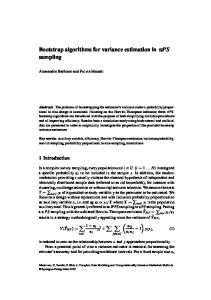
5.2. Variance Estimates of Major Industry-Level Raking Totals To compare the variance estimates for the domain-level raking-based totals, Figure 2 on the following pages shows plots of the ratio of the four raking alternatives for each variable of interest to the variance of the JKn right with 200 groups. In each plot, the 19 majors are sorted by descending total sample size (see Table 4). Figure 2. Ratio of Alternative Variance Estimates for Raking Totals to Jkn Right With 200 Groups, by Major Industry Gross Receipts 2.0 Binder JKn100 wrong

ratio to JKn200 right variance

Jkn200 wrong Jkn100 right

1.5

1.0

0.5

0.0 11

5

6

4

12

7

13

14

10

17

19

9

15

20

1

2

18

3

16

indy #

Net Depreciation 2.0 Binder JKn100 wrong

ratio to JKn200 right variance

Jkn200 wrong Jkn100 right

1.5

1.0

0.5

0.0 11

5

6

4

12

7

13

14

10

17 indy #

3699

19

9

15

20

1

2

18

3

16

Section on Survey Research Methods – JSM 2010

Figure 2. Alternative Estimated Coefficients of Variation of Major Industry-Level Totals – cont’d Net Income 2.0 Binder JKn100 wrong

ratio to JKn200 right variance

Jkn200 wrong Jkn100 right

1.5

1.0

0.5

0.0 11

5

6

4

12

7

13

14

10

17

19

9

15

20

1

2

18

3

16

indy #

Cost of Goods Sold 2.0 Binder JKn100 wrong Jkn200 wrong

1.5 ratio to JKn200 right variance

Jkn100 right

1.0

0.5

0.0

11

5

6

4

12

7

13

14

10

17

19

9

15

20

1

2

18

3

16

indy #

Depreciable Assets 2.0 Binder JKn100 wrong

ratio to JKn200 right variance

Jkn200 wrong Jkn100 right

1.5

1.0

0.5

0.0 11

5

6

4

12

7

13

14

10

17 indy #

3700

19

9

15

20

1

2

18

3

16

Section on Survey Research Methods – JSM 2010

Figure 2. Alternative Estimated Coefficients of Variation of Major Industry-Level Totals – cont’d Total Assets 2.0 Binder JKn100 wrong

ratio to JKn200 right variance

Jkn200 wrong Jkn100 right

1.5

1.0

0.5

0.0 11

5

6

4

12

7

13

14

10

17

19

9

15

20

1

2

18

3

16

indy #

Net Worth 2.0 Binder JKn100 wrong

ratio to JKn200 right variance

Jkn200 wrong Jkn100 right

1.5

1.0

0.5

0.0 11

5

6

4

12

7

13

14

10

17

19

9

15

20

1

2

18

3

16

indy #

Taxes After Credits 2.0 Binder JKn100 wrong

ratio to JKn200 right variance

Jkn200 wrong Jkn100 right

1.5

1.0

0.5

0.0 11

5

6

4

12

7

13

14

10

17 indy #

3701

19

9

15

20

1

2

18

3

16

Section on Survey Research Methods – JSM 2010

Figure 2. Alternative Estimated Coefficients of Variation of Major Industry-Level Totals – cont’d Total Receipts 2.0 Binder JKn100 wrong Jkn200 wrong

ratio to JKn200 right variance

1.5

Jkn100 right

1.0

0.5

0.0 11

5

6

4

12

7

13

14

10

17

19

9

15

20

1

2

18

3

16

1

2

18

3

16

indy #

Positive Income 2.0 Binder JKn100 wrong Jkn200 wrong Jkn100 right

ratio to JKn200 right variance

1.5

1.0

0.5

0.0 11

5

6

4

12

7

13

14

10

17

19

9

15

20

indy #

Deficit 2.0 Binder JKn100 wrong Jkn200 wrong

ratio to JKn200 right variance

1.5

Jkn100 right

1.0

0.5

0.0 11

5

6

4

12

7

13

14

10

17 indy #

3702

19

9

15

20

1

2

18

3

16

Section on Survey Research Methods – JSM 2010

In all plots, ratios equal to one indicate that a variance estimate is equivalent to the JKn right results with 200 replicate groups. We see that the alternative industry-level variance estimates are generally smaller than the JKn 200 right variance estimates, indicated by ratios less than one. This indicates that the Binder linearization method and implementing the jackknife incorrectly lead to smaller variance estimates. There generally is less of a difference for the JKn 100 right variance estimates. It is also difficult to discern any patterns related to the sample size, from larger industries on the left of each plot to the smaller industries on the right. 6. Conclusions We applied some alternative estimators of totals and their variances to data collected in SOI’s 2006 corporate sample. For our application, the post-stratification estimated totals (with poststrata defined by 72 industry groups) had larger variances than either the stratified estimator (with no poststratification or raking) or the raking estimator (with margins defined by design stratum and industry). For alternatives used to estimate the variance of totals under raking adjustments, generally the Binder Linearization and group jackknife with incorrectly formed replicate groups methods produced variance estimates that were both too small, despite having large sample sizes. References Binder, D. A. (1983). On the variances of asymptotically normal estimators from complex surveys. International Statistical Review, Vol. 51, pp. 279-292. Binder, D.A. and Theberge, A. (1988), "Estimating the Variance of Raking Ratio Estimators", Canadian Journal of Statistics, Vol. 16 Supplement, pp. 47-56. Brewer, K.R.W., Early, L.J., and Joyce, S.F. (1972), “Selecting Several Samples from a Single Population,” Australian Journal of Statistics, Vol. 14, pp. 231-239. Deville, J.C., Sarndal, C.E. (1992). “Calibration Estimators in Survey Sampling,” Journal of the American Statistical Association, Vol. 87, pp. 376-382. Deville, J.C., Sarndal, C.E. and, Sautory, O. (1993). “Generalized Raking Procedures in Survey Sampling.” Journal of the American Statistical Association, Vol. 88, pp. 1013-1020. Internal Revenue Service (2006), Statistics of Income–2006 Corporate Income Tax Returns, IRS, Publication 1053. Internal Revenue Service, Statistics of Income Bulletin, Winter 2008, Appendix A, “Description of the Sample and Limitations of the Data,” pp. 9-13. Internal Revenue Service (2010), Statistics of Income Bulletin, Winter 2010, Washington, D.C., pp. 215-217. Rao, J.N.K. and Shao, A.J. (1992). “Jackknife variance estimation with survey data under hot deck imputation,” Biometrika, Vol. 79, pp. 811-822. Research Triangle Institute (2008). SUDAAN Language Manual, Release 10.0, Research Triangle Park, NC: Research Triangle Institute. Oh, H. L. and Scheuren, F. J. (1987), "Modified Raking Ratio Estimation," Survey Methodology, Statistics Canada, Vol. 13, No. 2, pp. 209-219.

3703

Section on Survey Research Methods – JSM 2010

Yung, W. And Rao, J.N.K. (1996). Jackknife linearization variance estimators under stratified multi-stage sampling. Survey Methodology, 22, 23-31. Yung, W. and Rao, J.N.K. (2000). Jackknife variance estimation under imputation for estimators using post-stratification information. Journal of the American Statistical Association, Vol. 95, pp. 903-915. Valliant, R., Brick, M. J,, and Dever, J.A. (2008). "Weight Adjustments for the Grouped Jackknife Variance Estimator." Journal of Official Statistics, Vol. 24, No. 3, pp. 469-488. Valliant, R. (1993), “Poststratification and Conditional Variance Estimation,” Journal of the American Statistical Association, Vol. 88, No. 421, Theory and Methods, pp. 89- 96.

3704