alternative parameter estimation methods of the

ALTERNATIVE PARAMETER ESTIMATION METHODS OF THE CLASSICAL RYDBERG INTERATOMIC POTENTIAL by

Takalani N Malange A dissertation submitted in partial fulfillment of the requirements for the degree

MAGISTER TECHNOLOGIAE: MATHEMATICAL TECHNOLOGY in the Department of Mathematics and Statistics FACULTY OF SCIENCE

TSHWANE UNIVERSITY OF TECHNOLOGY Supervisor: Prof MY Shatalov Cosupervisor: Prof SV Joubert February 2016

"I hereby declare that this minidissertation submitted (in partial fulfillment) for the degree Magister Technologiae: Mathematical Technology at the Tshwane University of Technology is my own original work and has not previously been submitted to any other institution of higher education. I further declare that all sources cited, or quoted are indicated and acknowledged by means of a comprehensive list of references".

Takalani Malange

Copyright c Tshwane University of Technology 2015. ii

DEDICATION

I dedicate this work to my late mother, Masakona.

iii

ACKNOWLEDGEMENTS

I would like to acknowledge the following individuals and institution: •

Professor M.Y. Shatalov, my supervisor, for tangibly explaining the project, for his guidance and for sharing his knowledge.

•

Professor S.V. Joubert, my cosupervisor, for describing and specifying the changes necessary to make this shell document suitable for a TUT publication and for his guidance.

•

My sisters, Betty, Thanyani and Jeniffer, thank you so much for your unwavering love, support and encouragement.

•

Dr. C.R. Kikawa for going through the work and providing me with past research work for guidance.

•

The assistance of the staff of the department of mathematics and statistics as a whole is greatly appreciated.

•

Tshwane University of Technology for the scholarship.

iv

ABSTRACT

In this minidissertation the Rydberg interatomic potential function, which is a function of interatomic distance (r), is discussed and considered for parameter estimation. The parameters of the function are estimated using the proposed leastsquares methods, and experimental data sets of Copper (Cu), Silver (Ag) and CuAg alloy are used to investigate the performance of the methods. Since the Rydberg potential function is a nonlinear function, its parameter estimation requires several steps to transform it into a linear problem before applying the optimisation method of least squares. The least squares problems are then used to formulate goal functions which are minimised using numerical methods. Numerical solutions and graphical representations of the problems are obtained using a computer algebra system (CAS) and interpreted making use of graphical representations. The graphical representations generated using CAS are found to give a realistic description of the Rydberg interatomic potential function. The idea of estimating parameters of this function will be used in future research studies to approximate other interatomic potential functions.

v

TABLE OF CONTENTS

PAGE

DEDICATION . . . . . . . . . . . . . . . . . . . . . . . . . . . . . . . . . . . . . . . . . . . . . . . . . . . . . . . . . . . . . . . . . . . . . . . . . . . . iii ACKNOWLEDGEMENTS . . . . . . . . . . . . . . . . . . . . . . . . . . . . . . . . . . . . . . . . . . . . . . . . . . . . . . . . . . . . . . . . . iv ABSTRACT . . . . . . . . . . . . . . . . . . . . . . . . . . . . . . . . . . . . . . . . . . . . . . . . . . . . . . . . . . . . . . . . . . . . . . . . . . . . . . . v LIST OF TABLES . . . . . . . . . . . . . . . . . . . . . . . . . . . . . . . . . . . . . . . . . . . . . . . . . . . . . . . . . . . . . . . . . . . . . . . . vii LIST OF FIGURES . . . . . . . . . . . . . . . . . . . . . . . . . . . . . . . . . . . . . . . . . . . . . . . . . . . . . . . . . . . . . . . . . . . . . . viii Chapter 1 INTRODUCTION . . . . . . . . . . . . . . . . . . . . . . . . . . . . . . . . . . . . . . . . . . . . . . . . . . . . . . . . . . . . . . . . . . . . . . . . . 1.1 METHOD OF SOLUTION . . . . . . . . . . . . . . . . . . . . . . . . . . . . . . . . . . . . . . . . . . . . . . . . . . . . . . . . . 1.1.1.0 Lagrange multipliers . . . . . . . . . . . . . . . . . . . . . . . . . . . . . . . . . . . . . . . . . . . . . . . . . . . . . . 1.2 INTERATOMIC POTENTIALS . . . . . . . . . . . . . . . . . . . . . . . . . . . . . . . . . . . . . . . . . . . . . . . . . . . . 1.3 PROBLEM STATEMENT . . . . . . . . . . . . . . . . . . . . . . . . . . . . . . . . . . . . . . . . . . . . . . . . . . . . . . . . . . 1.4 OBJECTIVES . . . . . . . . . . . . . . . . . . . . . . . . . . . . . . . . . . . . . . . . . . . . . . . . . . . . . . . . . . . . . . . . . . . . . 1.5 MINIDISSERTATION LAYOUT . . . . . . . . . . . . . . . . . . . . . . . . . . . . . . . . . . . . . . . . . . . . . . . . . . .

1 2 2 3 4 4 4

Chapter 2 PARAMETER ESTIMATION OF THE CLASSICAL RYDBERG INTERATOMIC POTENTIAL USING DIFFERENTIAL METHODS . . . . . . . . . . . . . . . . . . . . . . . . . . . 5 2.1 INTRODUCTION . . . . . . . . . . . . . . . . . . . . . . . . . . . . . . . . . . . . . . . . . . . . . . . . . . . . . . . . . . . . . . . . . 5 2.2 METHODOLOGY . . . . . . . . . . . . . . . . . . . . . . . . . . . . . . . . . . . . . . . . . . . . . . . . . . . . . . . . . . . . . . . . . 6 2.2.1.0 Existing method of solution . . . . . . . . . . . . . . . . . . . . . . . . . . . . . . . . . . . . . . . . . . . . . . . . 6 2.2.2.0 Proposed method of solution . . . . . . . . . . . . . . . . . . . . . . . . . . . . . . . . . . . . . . . . . . . . . . . 6 2.2.2.1 Multiple goal functions method . . . . . . . . . . . . . . . . . . . . . . . . . . . . . . . . . . . . . . . . . . . . 7 2.2.2.2 "Minimization" method in Mathematica R . . . . . . . . . . . . . . . . . . . . . . . . . . . . . . . . . 11 2.3 RESULTS AND DISCUSSION . . . . . . . . . . . . . . . . . . . . . . . . . . . . . . . . . . . . . . . . . . . . . . . . . . . . 12 2.3.1.0 Results . . . . . . . . . . . . . . . . . . . . . . . . . . . . . . . . . . . . . . . . . . . . . . . . . . . . . . . . . . . . . . . . . . 12 2.3.2.0 Discussion . . . . . . . . . . . . . . . . . . . . . . . . . . . . . . . . . . . . . . . . . . . . . . . . . . . . . . . . . . . . . . . 16 Chapter 3 PARAMETER ESTIMATION OF THE CLASSICAL RYDBERG INTERATOMIC POTENTIAL USING INTEGRALDIFFERENTIAL METHODS . . . . . . . . . . . . . 17 vi

3.1 INTRODUCTION . . . . . . . . . . . . . . . . . . . . . . . . . . . . . . . . . . . . . . . . . . . . . . . . . . . . . . . . . . . . . . . . 3.2 METHODOLOGY . . . . . . . . . . . . . . . . . . . . . . . . . . . . . . . . . . . . . . . . . . . . . . . . . . . . . . . . . . . . . . . . 3.2.1.0 Existing method of solution . . . . . . . . . . . . . . . . . . . . . . . . . . . . . . . . . . . . . . . . . . . . . . . 3.2.2.0 Proposed method of solution . . . . . . . . . . . . . . . . . . . . . . . . . . . . . . . . . . . . . . . . . . . . . . 3.2.2.1 Multiple goal functions method . . . . . . . . . . . . . . . . . . . . . . . . . . . . . . . . . . . . . . . . . . . 3.2.2.2 "Minimization" method in Mathematica R . . . . . . . . . . . . . . . . . . . . . . . . . . . . . . . . . 3.3 RESULTS AND DISCUSSION . . . . . . . . . . . . . . . . . . . . . . . . . . . . . . . . . . . . . . . . . . . . . . . . . . . . 3.3.1.0 Results . . . . . . . . . . . . . . . . . . . . . . . . . . . . . . . . . . . . . . . . . . . . . . . . . . . . . . . . . . . . . . . . . . 3.3.2.0 Discussion . . . . . . . . . . . . . . . . . . . . . . . . . . . . . . . . . . . . . . . . . . . . . . . . . . . . . . . . . . . . . . .

17 17 17 18 18 23 24 24 28

Chapter 4 PARAMETER ESTIMATION OF THE CLASSICAL RYDBERG INTERATOMIC POTENTIAL USING INTEGRAL METHODS . . . . . . . . . . . . . . . . . . . . . . . . . . . . . . . 4.1 INTRODUCTION . . . . . . . . . . . . . . . . . . . . . . . . . . . . . . . . . . . . . . . . . . . . . . . . . . . . . . . . . . . . . . . . 4.2 METHODOLOGY . . . . . . . . . . . . . . . . . . . . . . . . . . . . . . . . . . . . . . . . . . . . . . . . . . . . . . . . . . . . . . . . 4.2.1.0 Existing method of solution . . . . . . . . . . . . . . . . . . . . . . . . . . . . . . . . . . . . . . . . . . . . . . . 4.2.2.0 Proposed method of solution . . . . . . . . . . . . . . . . . . . . . . . . . . . . . . . . . . . . . . . . . . . . . . 4.2.2.1 Multiple goal function method . . . . . . . . . . . . . . . . . . . . . . . . . . . . . . . . . . . . . . . . . . . . 4.2.2.2 "Minimization" method in Mathematica R . . . . . . . . . . . . . . . . . . . . . . . . . . . . . . . . . 4.3 RESULTS AND DISCUSSION . . . . . . . . . . . . . . . . . . . . . . . . . . . . . . . . . . . . . . . . . . . . . . . . . . . . 4.3.1.0 Results . . . . . . . . . . . . . . . . . . . . . . . . . . . . . . . . . . . . . . . . . . . . . . . . . . . . . . . . . . . . . . . . . . 4.3.2.0 Discussion . . . . . . . . . . . . . . . . . . . . . . . . . . . . . . . . . . . . . . . . . . . . . . . . . . . . . . . . . . . . . . .

29 29 29 29 29 31 37 37 37 41

Chapter 5 RESULTS AND DISCUSSION . . . . . . . . . . . . . . . . . . . . . . . . . . . . . . . . . . . . . . . . . . . . . . . . . . . . . . . . . . . . 42 5.1 RESULTS . . . . . . . . . . . . . . . . . . . . . . . . . . . . . . . . . . . . . . . . . . . . . . . . . . . . . . . . . . . . . . . . . . . . . . . . 42 5.2 DISCUSSION . . . . . . . . . . . . . . . . . . . . . . . . . . . . . . . . . . . . . . . . . . . . . . . . . . . . . . . . . . . . . . . . . . . . 45 Chapter 6 CONCLUSIONS AND RECOMMENDATIONS . . . . . . . . . . . . . . . . . . . . . . . . . . . . . . . . . . . . . . . . . . . 47 6.1 CONCLUSIONS . . . . . . . . . . . . . . . . . . . . . . . . . . . . . . . . . . . . . . . . . . . . . . . . . . . . . . . . . . . . . . . . . . 47 6.2 RECOMMENDATIONS FOR FURTHER RESEARCH . . . . . . . . . . . . . . . . . . . . . . . . . . . . . 47 REFERENCES . . . . . . . . . . . . . . . . . . . . . . . . . . . . . . . . . . . . . . . . . . . . . . . . . . . . . . . . . . . . . . . . . . . . . . . . . . . 48 Appendix: A

STRUCTURE OF A MINIDISSERTATION . . . . . . . . . . . . . . . . . . . . . . . . . . . . . . . 49

Appendix: B MATHEMATICA CODE . . . . . . . . . . . . . . . . . . . . . . . . . . . . . . . . . . . . . . . . . . . . . . . . . B.1 DIFFERENTIAL METHODS . . . . . . . . . . . . . . . . . . . . . . . . . . . . . . . . . . . . . . . . . . . . . . . . . . . . . B.2 INTEGRALDIFFERENTIAL METHODS . . . . . . . . . . . . . . . . . . . . . . . . . . . . . . . . . . . . . . . . . B.3 INTEGRAL METHODS . . . . . . . . . . . . . . . . . . . . . . . . . . . . . . . . . . . . . . . . . . . . . . . . . . . . . . . . . . B.4 COMPARISON OF METHODS . . . . . . . . . . . . . . . . . . . . . . . . . . . . . . . . . . . . . . . . . . . . . . . . . . .

vii

52 52 64 76 90

LIST OF TABLES

PAGE Table 2.1

Approximated parameter values. . . . . . . . . . . . . . . . . . . . . . . . . . . . . . . . . . . . . . . . 13

Table 3.1


Table 4.1


Table 5.1

Summary of used data. . . . . . . . . . . . . . . . . . . . . . . . . . . . . . . . . . . . . . . . . . . . . . . . 42

Table 5.2

Summary of approximated parameter values. . . . . . . . . . . . . . . . . . . . . . . . . . . . . . 43

Table 5.3

Optimisation of the Rydberg goal function using estimated parameters obtained from the differential, integraldifferential, integral and the builtin Mathematica methods of solution. . . . . . . . . . . . . . . . . . . . . . . . . . . . . . . . . . . . . . . 43

viii

LIST OF FIGURES

PAGE Figure 2.1

Estimated Rydberg potential energy curves (UU[r] and UUU[r]) fitted to Cu experimental data (U[r]) . . . . . . . . . . . . . . . . . . . . . . . . . . . . . . . . . . . . . . . . . . . . . 13

Figure 2.2

Potential energy curve of the error between the actual and estimated values of Copper . . . . . . . . . . . . . . . . . . . . . . . . . . . . . . . . . . . . . . . . . . . . . . . . . . . . . . . . . . 13

Figure 2.3

Estimated Rydberg potential energy curves (UU[r] and UUU[r]) fitted to Ag experimental data (U[r]) . . . . . . . . . . . . . . . . . . . . . . . . . . . . . . . . . . . . . . . . . . . . . 14

Figure 2.4

Potential energy curve of the error between the actual and estimated values of Silver . . . . . . . . . . . . . . . . . . . . . . . . . . . . . . . . . . . . . . . . . . . . . . . . . . . . . . . . . . . 14

Figure 2.5

Estimated Rydberg potential energy curves (UU[r] and UUU[r]) fitted to CuAg experimental data (U[r]) . . . . . . . . . . . . . . . . . . . . . . . . . . . . . . . . . . . . . . . . . . . . . 15

Figure 2.6

Potential energy curve of the error between the actual and estimated values of CopperSilver alloy. . . . . . . . . . . . . . . . . . . . . . . . . . . . . . . . . . . . . . . . . . . . . . . . . 15

Figure 3.1


Figure 3.2

Potential energy curve of the error between the actual and estimated values of Copper . . . . . . . . . . . . . . . . . . . . . . . . . . . . . . . . . . . . . . . . . . . . . . . . . . . . . . . . . . 25

Figure 3.3


Figure 3.4


Figure 3.5


Figure 3.6

Potential energy curve of the error between the actual and estimated values of CopperSilver alloy. . . . . . . . . . . . . . . . . . . . . . . . . . . . . . . . . . . . . . . . . . . . . . . . . 27

Figure 4.1


Figure 4.2

Potential energy curve of the error between the actual and estimated values of Copper . . . . . . . . . . . . . . . . . . . . . . . . . . . . . . . . . . . . . . . . . . . . . . . . . . . . . . . . . . 38 ix

Figure 4.3


Figure 4.4


Figure 4.5


Figure 4.6

Potential energy curve of the error between the actual and estimated values of CopperSilver alloy . . . . . . . . . . . . . . . . . . . . . . . . . . . . . . . . . . . . . . . . . . . . . . . . 40

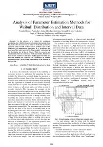
Figure 5.1

Comparision of the fitted potential energy curves of Cu using different methods of solution . . . . . . . . . . . . . . . . . . . . . . . . . . . . . . . . . . . . . . . . . . . . . . . . . . . . . . . . 43

Figure 5.2

Comparision of the fitted potential energy curves of Ag using different methods of solution . . . . . . . . . . . . . . . . . . . . . . . . . . . . . . . . . . . . . . . . . . . . . . . . . . . . . . . . 44

Figure 5.3

Comparision of the fitted potential energy curves of CuAg using different methods of solution . . . . . . . . . . . . . . . . . . . . . . . . . . . . . . . . . . . . . . . . . . . . . . . . 44

x

Chapter 1

INTRODUCTION

Parameter estimation has many practical uses that can be formulated as mathematical problems, for instance the shape of a can that minimises manufacturing costs; minimisation of the energy of a particle in physics; maximising the profit of the investments in economics; making production decisions that will maximise profits based on production capacity; optimising programs in science or design in engineering or in statistics to analyse data (Stewart, 2003, [1]). There are several parameter estimation methods for both linear and nonlinear problems. Estimation is achieved by the optimisation of problems, both constrained and unconstrained, and the aim of optimisation is to find an appropriate way to carry out functions. The type of method used when estimating parameters is dependent on the type of problem at hand (linear and nonlinear). Scientists and engineers are, however, often faced with the challenge of estimating the roots of nonalgebraic models that contain exponential and trigonometric functions, which are also known as transcendental functions (Burden, 2011, [2]). Parameter estimation involves the minimisation of an objective or goal function that should be optimised. Optimisation is achieved by differentiating the goal function with respect to all the unknowns, equating the differentials to zero and finding solutions for all unknowns. This study focusses on parameter estimation of the diatomic Rydberg interatomic potential function using the least squares method. This method involves minimisation of the sum of squares of differentiable functions to obtain acceptable parameter estimates. For a detailed discussion on parameter estimation see Englezos (2001,[3]). Differential calculus is mostly applied to optimisation problems, both constrained and unconstrained optimisation. The formulation of a parameter estimation problem is vital to the actual solution of the problem and constraints must be taken into consideration during problem formation. The derivative approach involves finding partial derivatives of the goal function and approximating the unknowns. The integral approach involves integrating the linear differential equation and then minimising it to obtain solutions. In reality constraints are encountered during optimisation of mathematical models and these can either be equality or inequality constraints. In such cases one must ensure that such constraints are satisfied for accuracy. 1

1.1

METHOD OF SOLUTION

Solving nonlinear systems is not an easy task that can be avoided by approximating the nonlinear system by a system of linear equations. Numerical methods of transcendental systems involve converting the integral functions into the linear systems of algebraic functions whose solutions can be obtained by using direct or iterative procedures. There are several methods that can be used for estimation. Nonlinear parameter estimation of models is usually achieved by curve fitting. The most common estimation method of model parameters is that of least squares that is applied to models that are nonlinear in nature, usually in engineering and science. The method involves minimisation of the objective function. Given N measurements of the output vector, parameters can be obtained by minimising the least squares objective function. Minimisation is achieved by differentiating the objective function with respect to the unknowns, equating the differentials to zero and finding solutions. When solving practical nonlinear least square problems methods like the GaussNewton, LevenbergMarquardt (LM) and Powell’s Dog Leg methods (see Maden, 2004, [4]) are usually applied, amongst others. Convergence of these methods is not guaranteed in some cases if the guess approximation to the iterative process is far from the optimal value. The method of solution in this study involves transforming the nonlinear Rydberg exponential function into a linear ordinary differential equation, setting up goal functions and solving their normal equations explicitly. Kikawa (2013, [5]) has discussed the idea of multiple goal functions to estimate parameters of the generalised Morse potential function. This work presents a comparison of parameter estimates between the least squares method using multiple goal functions and the more robust Mathematica R method.

1.1.1

Lagrange multipliers

Constrained optimisation has many practical uses that can be formulated as mathematical problems where the objective function, f (x), and the constraint, g(x), have specific meanings. Joseph Louis Lagrange (January 25, 1736 to April 10, 1813), who was known as one of the greatest mathematicians of the 18th century, was the first to develop today’s familiar method of finding extrema points of general functions using the Lagrange multiplier method (Thomas,1996, [6]). Lagrange Multipliers are mathematical tools for constrained optimisation of differentiable functions. Many computational programming methods, such as the barrier and interior point method (in electrical engineering) have been developed based on the basic rules of the Lagrange

2

multipliers method (Bertsekas, 2003,[7]). This method may be applied to both equality and inequality constraints and has proven to be a powerful technique for solving nonlinear optimisation problems (Larson, 2007, [8]). Lagrange multipliers were initially used only in problems with equality constraints (Rockafellar, 1993, [9]) before being used on inequality constraints. The Lagrange multipliers method is based on setting up a new function, the Lagrangian function, L(x, λ) = f (x) − λg(x), where λ is the Lagrange multiplier, x is the vector of unknown parameters and L(x, λ) is the function to be minimised or maximised. The idea of the Lagrange multiplier is used in this study to approximate unknown parameters.

1.2

INTERATOMIC POTENTIALS

Interatomic potential functions describe interactions between atoms during chemical reactions. Almost all physical phenomena can be attributed to repulsive and attractive forces between atoms that require weighing over a number of events. Interatomic potential functions describe how the potential energy, U(r), of a system of N atoms depend on the coordinates of the atoms, rk , where k = 1, . . . , N. The Rydberg function is used in physics to characterise the wavelengths of reactive elements, and was formulated by Johannes Robert Rydberg (November 8, 1854 – December 28, 1919). For binding to occur, the potential must have both attraction and repulsion components. There are different forms of interatomic potentials which exist and the following factors should be considered when choosing a potential for practical use: •

accuracy (reproduce properties of interest accurately)

•

transferability (study a variety of properties not designed for)

•

computational speed (fast computations)

The choice of potential to use is dependent on the area of interest. Accuracy is required in computational chemistry, while computational speed is required in materials science. For a more detailed discussion on interatomic potentials refer to Rieth (2003, [10]) and Torrens (1973, [11]). Interatomic potentials are analysed by plotting potential energy curves. A potential energy curve is a mathematical tool that plots the energy of a molecule as a model of its geometry. An analysis of potential energy curves gives a better understanding of material properties, which are predicted based on attractive and repulsive forces that bind atoms together, and are consequently used in data analysis. Potential energy curves are widely used in science and engineering to study material properties. They have a welldepth magnitude that indicates the strength of the molecule bond 3

(the steeper the well the more stable the molecule) and the dissociation energy of molecules. For a more detailed analysis of potential energy curves and material properties, refer to Callister (2007, [12]).

1.3

PROBLEM STATEMENT

Transcendental functions are often solved by linearisation procedures. Consider the Rydberg interatomic potential function (Lim, 2004, [13]), U (r), U (r) = −D(1 + αr)e−αr ,

(1.1)

where D is the minimum potential welldepth magnitude, α is the steepness of the potential and r is the corresponding interatomic distance. Equation (1.1) can be rewritten as U (r) = Ae−αr + Bre−αr = (A + Br) e−αr .

(1.2)

Comparing Equations (1.1 and 1.2) it is observed that A = −D

and

B = −αD.

The research problem is to develop methods of parameter estimation for model (1.2) that do not require the use of initial guess values.

1.4

OBJECTIVES

The primary objective of this study is to explicitly estimate the parameters of Equation (1.2) by converting the transcendental leastsquares model into a linear leastsquares problem that is linear with respect to unknown parameters using a computer algebra system.

1.5

MINIDISSERTATION LAYOUT

Chapters 2, 3 and 4 respectively show parameter estimations of the Rydberg interatomic potential using the leastsquares method and differential, integraldifferential and integral methods. In Chapter 5, results from Chapters 2, 3 and 4 are compared and discussed. Chapter 6 presents the findings of the minidissertation together with the recommendations for future research.

4

Chapter 2 PARAMETER ESTIMATION OF THE CLASSICAL RYDBERG INTERATOMIC POTENTIAL USING DIFFERENTIAL METHODS

Parameter estimation is an important aspect in estimation and distribution theory. This Chapter deals with parameter estimation of the Rydberg interatomic potential function using differential methods. Interatomic potentials describe interactions between atoms during chemical reactions of metals and nonmetals. The Rydberg interatomic potential function is a function characterised by interatomic distance, r, and other parameters (see Equation 2.1). The proposed method is tested based on the experimental data of Copper (Cu), Silver (Ag) and CopperSilver alloy as found by Mishin (2006, [14], [15] and [16]). The estimated parameters obtained from different methods were used to construct potential energy curves which were analysed and fitted to the experimental data sets for the CuCu, AgAg and CuAg molecules.

2.1

INTRODUCTION

This section studies the classical Rydberg interatomic potential function, which is an algebraic combination of two exponential functions with three unknown parameters. The Rydberg function (2.1) is used in physics to characterise the wavelengths of reactive elements. Existing parameter estimation methods require initial guess values to approximate solutions. The method of solution proposed in this Chapter has the advantage that it does not require initial guess values. The method involves the transformation of the nonlinear Rydberg potential function, Equation (2.1), into a linear second order differential equation, Equation (2.8), with constant coefficients before applying the optimization method of ordinary leastsquares to approximate unknown parameters A, B and α. The results from the proposed method of solution will be compared to the results from the "Minimization" method contained in Mathematica

R

. Potential energy curves were

constructed using experimental data sets and then reconstructed using results obtained from the methods of solution. Both methods produced comparable estimates with respect to the experimental data obtained.

5

2.2

2.2.1

METHODOLOGY

Existing method of solution

In this section the classical Rydberg interatomic potential function U (r) = Ae−αr + Bre−αr = (A + Br) e−αr ,

(2.1)

is examined, where A, B and α are the model parameters to be estimated and r is the interatomic distance. Assuming that experimental data set {rk , Uk = U(rk )} with k = 1, . . . , N where N is the number of experimental points available, a goal function to approximate the Rydberg constants, A, B and α is formulated as, 1 G(A, B, α) = 2

N

k=1

Ae−αrk + Brk e−αrk − Uk

2

.

(2.2)

Partial derivatives of Equation (2.2) with respect to A, B and α are ∂G = ∂A ∂G = ∂B ∂G = ∂α

N

k=1 N

k=1 N

k=1

Ae−αrk + Brk e−αrk − Uk e−αrk = 0,

(2.3)

Ae−αrk + Brk e−αrk − Uk rk e−αrk = 0,

(2.4)


(2.5)

−Ae−αrk − Brk e−αrk = 0.

It can be noted that Equations (2.3, 2.4 and 2.5) cannot be solved explicitly to give exact solutions. Existing parameter estimation methods require initial guess values to approximate solutions that can lead to time lags or even nonconvergence if they are far from optimal solutions.

2.2.2

Proposed method of solution

Consider function (2.1), which is the general solution of some ordinary differential equation of order two that is linear with respect to the unknown parameter α d2 U dU + α2 U = 0, + 2α 2 dr dr whose characteristics equation is (λ + α)2 = 0.

(2.6)

(2.7)

Presenting Equation (2.6) as dU d2 U + bU = 0, (2.8) +a 2 dr dr where a and b are new unknown parameters depending on α. From Equation (2.6 and 2.8) it is

6

deduced that b = α2 ,

(2.9)

g(a, b) = a2 − 4b = 0.

(2.10)

a = 2α and hence the constraint can be formulated as

2.2.2.1

Multiple goal functions method

Two goal functions were constructed using the least squares method and experimental data sets by Mishin (2006, [14], [15] and [16]). The first goal function is formulated to estimate a, b, λ and hence α. The second goal function is formulated to estimate the unknown Rydberg constants A ˜ and B. The parameters to be estimated are represented as α ˜ , A˜ and B. The first goal function, G1 (a, b, λ) Considering the Rydberg function with data sets k = 1, . . . , N where N is the number of experimental points, a goal function to estimate a, b and λ is formulated using the leastsquares method to minimise Equation (2.8) subject to the constraint in Equation (2.10) as 1 G1 (a, b, λ) = 2

N

k=1

dUk d2 Uk +a + bUk 2 drk drk

2

+ λ a2 − 4b .

(2.11)

Partial derivatives of Equation (2.11) with respect to a, b and λ are

∂G1 = ∂a ∂G1 = ∂b

N

k=1 N

k=1

dUk d2 U k +a + bUk 2 drk drk

d2 U k dUk +a + bUk Uk − 4λ, 2 drk drk

∂G1 = a2 − 4b. ∂λ ∂G1 ∂G1 ∂G1 = 0, = 0 and = 0 yields Setting ∂a ∂b ∂λ N d2 Uk dUk +a + bUk 2 dr dr k k k=1 N

k=1

dUk + 2λa, drk

(2.12) (2.13) (2.14)

dUk + 2λa = 0, drk

(2.15)

d2 U k dUk +a + bUk Uk − 4λ = 0, 2 drk drk

(2.16)

a2 − 4b = 0.

(2.17)

7

Presenting Equation (2.15 and 2.16) in matrix form   2 N dUk dUk 2λ + N U k=1 drk k=1 k drk  a  N N 2 dUk b U (U ) k

k=1

k=1

drk

k



=

− 4λ −

N dUk d2 Uk k=1 drk drk2 N d2 Uk k=1 Uk drk2



.

(2.18)

Since λ is unknown Equation (2.18) can be written as a(λ) b(λ)



=

N k=1

2λ + N k=1

Uk

dUk drk

2

N k=1

k Uk dU drk N 2 k=1 (Uk )

dUk drk

−1  



− 4λ −

N dUk d2 Uk k=1 drk drk2 N d2 Uk k=1 Uk drk2



 . (2.19)

The constraint, in Equation (2.10), can be rewritten as (a(λ))2 − 4b(λ) = 0,

(2.20)

Equation (2.20) is used to estimate the value of λ, hence calculate a and b using Equation (2.19). Form I: Copper atom Using the pair interactions of the Copper atom by Mishin (2006, [14]), the following can be approximated (see Appendix B.1).  a(λ) b(λ)

 = 

96305.312 + 76.151(−274.925 + 4λ) 13309.156 + 42.390λ 346008.618 + (901.53 + 2λ)(−274.925 + 4λ) 13309.156 + 42.390λ

Substituting the solution in Equation (2.21) into Equation (2.20) 2  346008.618 + (901.53 + 2λ) 96305.312 + 76.151  (−274.925 + 4λ)   (−274.925 + 4λ)     (13309.156 + 42.390λ)  − 4  (13309.156 + 42.390λ) 

solving Equation (2.22) results in

λ = −315.47 − 30.8527i;

−315.47 + 30.8527i;





 . 

  = 0, 

3.33921,

(2.21)

(2.22)

(2.23)

hence the real solution of Equation (2.23) is, λ = 3.339,

(2.24)

substituting the solution in (2.24) into Equation (2.21) a b

5.679 8.063

=

.

(2.25)

The values of a and b satisfy the constraint in Equation (2.10) a2 − 4b = 0, 8

(2.26)

where α can be calculated from Equation (2.9) a √ α ˜ = = b = 2.840. 2

(2.27)

Form II: Silver atom Using the pair interactions of the Silver atom by Mishin (2006, [15]), the following unknowns can be calculated using Mathematica  a(λ) b(λ)

 = 

R

(see Appendix B.1). 

1268.314 + 1.469(50.987 + 4λ) 195.580 + 18.019λ 206.835 + (21.948 + 2λ) (50.987 + 4λ) 195.580 + 18.019λ

 . 

Substituting the solutions in (2.28) into Equation (2.20) 2  1268.314 + 1.469 206.835 + (21.948 + 2λ)  (50.987 + 4λ)   (50.987 + 4λ)     195.580 + 18.019λ  − 4  195.580 + 18.019λ 

solving Equation (2.29)

λ = −18.5994 − 12.236i;

−18.5994 + 12.236i;

(2.28)



  = 0, 

2.68367,

(2.29)

(2.30)


(2.31)

substituting the solution in Equation (2.31) into Equation (2.28) a 5.571 = . b 7.759 The values of a and b satisfy the constraint in Equation (2.10)

(2.32)

a2 − 4b = 0,

(2.33)

where α can be calculated from Equation (2.9) as a √ α ˜ = = b = 2.786. 2

(2.34)

Form III: CopperSilver alloy Using the pair interactions of the CopperSilver alloy by Mishin (2006, [16]), the following unknowns can be calculated using Mathematica R (see Appendix B.1).  92944.606 + 85.5338 (−395.526 + 4λ)  a(λ) 10023.287 + 40.265λ =  394882.260 + (861.267 + 2λ) (−395.526 + 4λ) b(λ) 10023.287 + 40.265λ 9



 . 

(2.35)

Substituting the solutions in Equation (2.35) into Equation (2.17) 2  92944.606 + 85.5338 394882.260 + (861.267 + 2λ)  (−395.526 + 4λ)   (−395.526 + 4λ)     (10023.287 + 40.265λ)  − 4  (10023.287 + 40.265λ) 



  = 0, 

(2.36)

solving Equation (2.36) λ = −252.701 − 44.4735i;

−252.701 + 44.4735i;

15.5639,

(2.37)


(2.38)

substituting the solution in Equation (2.38) into Equation (2.35) a 6.051 = . b 9.152 The values of a and b satisfy the constraint in Equation (2.10)

(2.39)

a2 − 4b = 7.105 × 10−15 ∼ = 0,

(2.40)

where α ˜ can be calculated from Equation (2.9) as a √ α ˜ = = b = 3.025. 2

(2.41)

˜ B), ˜ The second goal function, G2 (A, ˜ is formulated as, The goal function to estimate A˜ and B ˜ B) ˜ = G2 (A,

1 2

N

k=1

˜ k e−˜αrk − Uk ˜ −˜αrk + Br Ae

2

,

(2.42)

˜ are partial derivatives of Equation (2.42) with respect to the unknown parameters A˜ and B ∂G2 = ∂ A˜

N

k=1 N

˜ −˜αrk + Br ˜ k e−˜αrk − Uk e−˜αrk = 0, Ae

(2.43)

∂G2 ˜ −˜αrk + Br ˜ k e−˜αrk − Uk rk e−˜αrk = 0, Ae = ˜ ∂B k=1 writing Equations (2.43 and 2.44) in matrix form N −˜ αrk 2 k=1 e N −˜ αrk 2 k=1 rk e

N −˜ αrk 2 k=1 rk e N −˜ αrk 2 k=1 rk e

A˜ ˜ B

=

N k=1 Uk N k=1 Uk

e−˜αrk rk e−˜αrk

(2.44)

,

(2.45)

thus A˜ ˜ B

=

N −˜ αrk 2 k=1 e N −˜ αrk 2 k=1 rk e


10

−1

N k=1 Uk N k=1 Uk


.

(2.46)

Using experimental data by Mishin (2006, [14], [15] and [16]), the unknown parameters A and B can be approximated using Mathematica R (see Appendix B.1). Form I: Copper atom

A˜ ˜ B

2058.427 −903.918

=

.

(2.47)

Substituting the results in Equation (2.47 and 2.27) into Equation (1.2) ˜ e−˜αr = (2058.440 − 903.924r) e−2.840r . U(r) = A˜ + Br Form II: Silver atom

A˜ ˜ B

4991.876 −1886.726

=

.

(2.48)

Substituting the results in Equation (2.48 and 2.34) into Equation (1.2) ˜ e−˜αr = (1336.924 − 506.422r) e−2.786r . U(r) = A˜ + Br

(2.49)

Form III: CopperSilver alloy A˜ ˜ B

5257.618 −2122.751

=

(2.50)

Substituting the results in Equation (2.50 and 2.41) into Equation (1.2) ˜ e−˜αr = (5257.618 − 2122.750r) e−3.025r . U (r) = A˜ + Br

2.2.2.2

(2.51)

"Minimization" method in Mathematica R

Computer Algebra Systems have builtin methods for solving transcendental models. Using the buildin "Minimize" function in Mathematica

R

(see Appendix B.1) to minimise Equation (2.2)

results in the following: Form I: Copper atom



   A˜ 1513.835  B ˜  =  −663.335  . 2.719 α ˜

(2.52)

Substituting the results in Equation (2.52) into Equation (1.2) ˜ e−˜αr = (1513.835 − 663.335r) e−2.719r . U(r) = A˜ + Br 11

(2.53)

Form II: Silver atom

   A˜ 777.002  B ˜  =  −302.134  . 2.268 α ˜ 

(2.54)

Substituting the results in Equation (2.54) into Equation (1.2) ˜ e−˜αr = (2326.580 − 885.148r) e−2.557r . U(r) = A˜ + Br Form III: CopperSilver alloy

(2.55)

   1050.418 A˜  B ˜  =  −419.046  . 2.426 α ˜

(2.56)

˜ e−˜αr = (1050.418 − 419.046r) e−2.426r . U(r) = A˜ + Br

(2.57)



Substituting the results in Equation (2.56) into Equation (1.2)

The builtin "Minimize" function in Mathematica

R

did not require initial guess values in this

case to minimise our goal function, which is not the case in other CAS such as Mathcad. In such cases one can use the multiple goal function method to calculate initial guess values that can further be used to approximate parameters.

2.3

RESULTS AND DISCUSSION

The Rydberg interatomic potential function (see Equation 1.2) is an algebraic combination of two exponential functions with three unknown parameters, A, B and α, which were estimated from experimental data sets by Mishin (2006, [14], [15] and [16]). The parameters were estimated using the leastsquares method via multiple goal functions and the builtin "Minimize" function contained in Mathematica R .

2.3.1

Results

Data sets by Mishin (2006) were used to generate potential energy curves and then fitted to the estimated Rydberg potential functions for the CuCu, AgAg and CuAg molecules (see Figures 2.1, 2.3 and 2.5) using the different methods of solution. Table (2.1) shows estimated parameters using the differential method and the builtin Mathematica

R

method. Figures (2.1,

2.3 and 2.5) show the plots of the actual and estimated potential energy curves of CuCu, AgAg 12

and CuAg respectively, while Figures (2.2, 2.4 and 2.6) show the graphical representations of the errors between the plots. For simplicity the actual plot will be represented as U (r), the first approximation using the differential methods as UU (r) and the mathematica leastsquares approximation as U UU (r). Table 2.1: Approximated parameter values. Parameter Cu Ag CuAg

Differential method ˜ A˜ B 2058.427 −903.918 4991.876 −1886.726 5257.618 −2122.751

α ˜ 2.840 2.786 3.025

Builtin Mathematica R ˜ A˜ B 1513.835 −663.335 777.002 −302.134 1050.418 −419.046

method α ˜ 2.719 2.268 2.426

Form I: Copper atom

Figure 2.1: Estimated Rydberg potential energy curves (UU[r] and UUU[r]) fitted to Cu experi mental data (U[r]) with error

Figure 2.2: Potential energy curve of the error between the actual and estimated values of Copper 13


Figure 2.3: Estimated Rydberg potential energy curves (UU[r] and UUU[r]) fitted to Ag experi mental data (U[r]) with error

Figure 2.4: Potential energy curve of the error between the actual and estimated values of Silver

14

Form III: CopperSilver alloy

Figure 2.5: Estimated Rydberg potential energy curves (UU[r] and UUU[r]) fitted to CuAg exper imental data (U[r]) with error

Figure 2.6: Potential energy curve of the error between the actual and estimated values of Cop perSilver alloy.

15

2.3.2

Discussion

For this study experimental data sets by Mishin were used to construct potential energy curves for the different atoms and then reconstructed using the estimated parameters. The choice in the solution of the Lagrangian multiplier (λ) is of paramount importance as the accuracy of estimates is dependant on λ. Three solutions were obtained in all instances (see Appendix B), two of the solutions were complex leaving only one real root, which was then chosen to approximate a and b. The potential energy curves constructed using results of the estimated parameters presented seem to fit the experimental data sets for the CuCu, AgAg and CuAg molecules (see Figures 2.2, 2.4 and 2.6). Both these methods produced comparable estimates of the parameters (see Table 2.1 and Figures 2.2, 2.4 and 2.6) and have the advantage that they do not require guess values to estimate solutions. The results for the Cu atom were very satisfactory as compared to both the Ag atom and the CuAg alloy (see Figures 2.2, 2.4 and 2.6). Results using the "Minimize" option in Mathematica R is more accurate than the results obtained by the proposed method of multiple goal functions. The variation in performance of the methods may be explained by the fact that the experimental data was numerically differentiated twice, introducing errors in the computational process as a result.

16

Chapter 3

PARAMETER ESTIMATION OF THE CLASSICAL RYDBERG INTERATOMIC POTENTIAL USING INTEGRALDIFFERENTIAL METHODS

This Chapter is concerned with parameter estimation of the Rydberg interatomic potential function using integraldifferential methods. The proposed method is tested using experimental data of Copper (Cu), Silver (Ag) and CopperSilver alloy by Mishin (2006, [14], [15] and [16]). The estimated parameters obtained from the least squares methods were used to construct potential energy curves which were analysed and fitted to the experimental data sets for the CuCu, AgAg and CuAg molecules.

3.1

INTRODUCTION

The method of solution in this chapter has the advantage that it does not require initial guess values like the differential method described in Chapter 2. The method involves the transformation of the nonlinear Rydberg potential function, Equation (2.1), into a linear second order differential equation, Equation (3.3), and integrating it, thus making it an integraldifferential equation (see Equation (3.7)) before applying the optimization method of ordinary leastsquares to approximate A, B and α. The results from the proposed method of solution is compared to the results from the "Minimization" method contained in Mathematica R as in Chapter 2. Potential energy curves were constructed using experimental data sets and then reconstructed using results obtained from the methods of solution. Both methods produced satisfactory estimates.

3.2

3.2.1

METHODOLOGY


The current methods of solution have already been discussed in Chapter 2 subsection 2.2.1. We proceed to the fomulation of the proposed method.

17

3.2.2


Consider Equation (2.1), which is the general solution of the ordinary differential equation that is linear with respect to the unknown parameter α dU d2 U + 2α + α2 U = 0, 2 dr dr whose characteristics equation is (λ + α)2 = 0.

(3.1)

(3.2)

Equation (3.1) can be rewritten as dU d2 U +a + bU = 0, (3.3) 2 dr dr where a and b are new unknown parameters depending on α. From Equation (3.1 and 3.3) it is deduced that a = 2α and

b = α2 .

(3.4)

The following constraint can be fomulated from Equation (3.1 and 3.3) g(a, b) = a2 − 4b = 0. Integrating Equation (3.1) with respect to r, over the interval [r0 , r] results in r d2 U dU + a + bU dρ = 0, dr2 dr r0 or r dU(r) dU (r0 ) U (ρ)dρ = 0, − + a (U (r) − U (r0 )) + b dr dr r0 letting r dU (r0 ) dU (r) U(ρ)dρ = U ′; − − aU(r0 ) = c; and I1 = dr dr r0 and rearranging Equation (3.7) results in U ′ + aU + bI1 + c = 0,

(3.5)

(3.6)

(3.7)

(3.8)

(3.9)

where c is the new unknown parameter.

3.2.2.1

Multiple goal functions method

Two goal functions were constructed using the least squares method and experimental data sets by Mishin (2006, [14], [15] and [16]). The first goal function as in Chapter 3 is formulated to estimate a, b, c, λ and hence α, the second goal function is formulated to estimate the unknown Rydberg constants A and B.

18

The first goal function, G1 (a, b, λ) Considering the Rydberg interatomic potential function with data sets k = 1, . . . , N where N is the number of experimental points, a goal function to estimate a, b, c and λ is formulated, using the leastsquares method to minimise Equation (3.9) subject to the constraint in Equation (2.10) as

N

1 2 (U ′ + aUk + bI1k + c) + λ a2 − 4b . 2 k=1 k Partial derivatives of Equation (3.10) with respect to a, b, c and λ are G1 (a, b, c, λ) =

∂G1 = ∂a ∂G1 = ∂b ∂G1 = ∂c

(3.10)

N

(Uk′ + aUk + bI1k + c) Uk + 2λa,

(3.11)

(Uk′ + aUk + bI1k + c) I1k − 4λ,

(3.12)

(Uk′ + aUk + bI1k + c) ,

(3.13)

k=1 N

k=1 N

k=1

∂G1 = a2 − 4b. ∂λ ∂G1 ∂G1 ∂G1 Expanding and setting = 0, = 0 and = 0 yields ∂a ∂b ∂c N

N

(Uk )2 + 2λ

a

k=1 N

I1k Uk + c k=1

k=1

N

Uk′ I1k − 4λ = 0,

(3.16)

N

(I1k )2 + c

I1k + k=1

N

k=1 N

N

Uk + b

a

(3.15)

k=1

N

k=1

Uk′ Uk = 0,

Uk + k=1

N

Uk Ik + b

a

N

+b

(3.14)

k=1

Uk′ = 0.

I1k + N c + k=1

(3.17)

k=1

Rewriting Equation (3.15, 3.16 and 3.17) in matrix form     N 2 N N (U ) + 2λ I U U − a k k=1 k=1 k k k=1 k     N N 2 N   b = 4λ − k=1 Uk I1k k=1 (I1k ) k=1 I1k N N c − N k=1 Uk k=1 I1k

N ′ k=1 Uk Uk N ′ k=1 Uk I1k N ′ k=1 Uk



 , (3.18)

thus, 





a  b =  c

N 2 k=1 (Uk ) + 2λ N k=1 Uk I1k N k=1 Uk

N k=1 Ik Uk N 2 k=1 (I1k ) N k=1 I1k

N k=1 Uk N k=1 I1k

N

and the constraint (see Equation (3.5)) can be rewritten as (a(λ))2 − 4b(λ) = 0. 19

−1   

−  4λ − −

N ′ k=1 Uk Uk N ′ k=1 Uk I1k N ′ k=1 Uk



 , (3.19) (3.20)

Equation (3.20) will be used to estimate the value of λ, therefore calculate a, b and c using Equation (3.19). Form I: Copper atom Using the pair interactions of the Copper atom by Mishin (2006, [14]) the following can be approximated (see Appendix B.2).     a(λ)   b(λ)  =    c(λ)  

985574.5 + 1111.44(21.0695 + 4λ) 179078.1 + 21028.6λ 84636.6 + 302.085(2201.64 + 250.933λ) + (21.0695 + 4λ)(27896.5 + 3262λ) 1790781.1 + 21028.6λ 46611.5 + 302.085(309.817 + 32.1964λ) + (21.0695 + 4λ)(2201.64 + 250.933λ) 1790781. + 21028.6λ (3.21)

Substituting the solutions in Equation (3.21) into Equation (3.20) 2  84636.6 + 302.085(2201.64 + 250.933λ) 985574.5 + 1111.44   +(21.0695 + 4λ)(27896.5 + 3262λ)  (21.0695 + 4λ)     (179078.1 + 21028.6λ)  − 4  (1790781.1 + 21028.6λ) 

Solving Equation (3.22) results in

λ = −14.167 − 8.162i;

−14.166 + 8.162i;

0.205



  = 0. (3.22)  (3.23)

hence the real solution of Equation (3.23) is, λ = 0.205. Substituting the solution in Equation (3.24) into Equation (3.21) results in     a 5.507  b  =  7.582  . c 1.044 The values of a and b satisfy the constraint in Equation (3.5) a2 − 4b = 0, and where α can be calculated from Equation (3.4) a √ α ˜ = = b = 2.754. 2

(3.24)

(3.25)

(3.26)

(3.27)

Form II: Silver atom Using the pair interactions of the Silver atom by Mishin (2006, [15]), the following can be approximated (see Appendix B.2). 20



   .   



   a(λ)   b(λ)  =    c(λ)  

−18447.6 + 3576.91(8.26381 + 4λ) 1986.15 + 8216.19λ 5255.35 − 35.766(666.747 + 292.529λ) + (8.26381 + 4λ)(3742.92 + 2600λ) 1986.15 + 8216.19λ 1005.76 − 35.766(123.552 + 39.2328λ) + (8.26381 + 4λ)(666.747 + 292.529λ) 1986.15 + 8216.19λ (3.28)



   .   

Substituting the solutions in Equation (3.28) into Equation (3.20) 

2  5255.35 − 35.766(666.747 + 292.529λ) −18447.6 + 3576.91    (8.26381 + 4λ)  +(8.26381 + 4λ)(3742.92 + 2600λ)    (1986.15 + 8216.19λ)  − 4  (1986.15 + 8216.19λ)



  = 0, 

(3.29)

solving Equation (3.29) λ = −1.560;

−0.655;

0.073.

(3.30)

Letting, λ = 0.073,

(3.31)

since the solution in Equation (3.31) yields a minimum constraint (see Appendix B.2) and substituting Equation (3.31) into Equation   (3.28)  results in a 4.702  b  =  5.528  . 0.917 c The values of a and b satisfy the constraint in Equation (3.5) a2 − 4b = −1.06581 × 10−14 ∼ = 0, where α can be calculated from Equation (3.4) as a √ α ˜ = = b = 2.351. 2

(3.32)

(3.33)

(3.34)

Form III: CopperSilver alloy Using the pair interactions of the CopperSilver alloy by Mishin (2006, [16]), the following can be approximated (see Appendix B.2). 

   a(λ)   b(λ)  =    c(λ)  

2.06977 × 106 + 2048.21(20.0049 + 4λ) 365186. + 41891.9λ 175191.97 + 337.895(3181.43 + 355.719λ) + (20.0049 + 4λ)(43804.5 + 5002λ) 365186. + 41891.9λ 70418.7 + 337.895(398.899 + 42.0471λ) + (20.0049 + 4λ)(3181.43 + 355.719λ) 365186. + 41891.9λ (3.35)

21



   .   

Substituting the solutions in Equation (3.35) into Equation (3.20)  2 175191.97 + 337.895(3181.43 + 355.719λ) 2.06977 × 106 + 2048.21    +(20.0049 + 4λ)(43804.5 + 5002λ) (20.0049 + 4λ)     (365186. + 41891.9λ)  − 4  (365186. + 41891.9λ) 



  = 0, 

(3.36)

solving Equation (3.36) λ = −14.8864 − 9.25501i;

−14.8864 + 9.25501i;

1.3095

(3.37)

hence the real solution of Equation (3.37) is, λ = 1.310.

(3.38)

   a 5.051  b  =  6.377  . c 0.752

(3.39)

Substituting (3.38) into Equation (3.35) 

The values of a and b satisfy the constraint in Equation (3.5) a2 − 4b = −7.10543 × 10−15 ,

(3.40)


(3.41)

The second goal function, G2 (A, B), ˜ is formulated as, The goal function to estimate A˜ and B ˜ B) ˜ =1 G2 (A, 2

N

k=1

˜ −˜αrk + Br ˜ k e−˜αrk − Uk Ae

2

,

(3.42)

partial derivatives of Equation (3.42) with respect to A and B are, ∂G2 = ∂ A˜ ∂G2 = ∂B

N

k=1 N

k=1

˜ −˜αrk + Br ˜ k e−˜αrk − Uk e−˜αrk = 0, Ae

(3.43)

˜ −˜αrk + Br ˜ k e−˜αrk − Uk rk e−˜αrk = 0, Ae

(3.44)

writing Equation (3.43 and 3.44) in matrix form N −˜ αrk 2 k=1 e N −˜ αrk 2 k=1 rk e


A˜ ˜ B

thus 22

=

N k=1 Uk N k=1 Uk


,

(3.45)

A˜ ˜ B

=

N −˜ αrk 2 k=1 e N −˜ αrk 2 k=1 rk e


−1

N k=1 Uk N k=1 Uk


.

(3.46)

Using experimental data by Mishin (2006, [14], [15] and [16]) A and B can be approximated using Mathematica R (see Appendix B.2). Form I: Copper (Cu) atom

A˜ ˜ B

1652.750 −724.661

=

.

(3.47)

Substituting the results in Equation (3.47 and 3.27) into the Rydberg interatomic function in Equation (2.1) ˜ e−˜αr = (1652.750r − 724.661) e−2.754r . U(r) = A˜ + Br Form II: Silver (Ag) atom

A˜ ˜ B

1063.382 −410.753

=

.

(3.48)

(3.49)

Substituting the results in Equation (3.49 and 3.34) into the Rydberg interatomic function in Equation (2.1) ˜ e−˜αr = (1063.382 − 410.753r) e−2.351r . U(r) = A˜ + Br

(3.50)


1382.832 −552.950

=

.

(3.51)

Substituting the results in Equation (3.51 and 3.41) into the Rydberg interatomic function in Equation (2.1) ˜ e−˜αr = (1382.832 − 552.950r) e−2.525r . U(r) = A˜ + Br

3.2.2.2

(3.52)


Computer Algebra Systems have builtin methods for solving transcendental models. Using the buildin "Minimize" function in Mathematica

R

(see Appendix B.2) to minimise Equation (3.42),

we obtained the same numerical results as those obtained in Chapter 2 subsection 2.2.2.2 since the method of solution used is the same. We subsequently proceed to the results and discussion section.

23

3.3


The unknown parameters, A, B and α, of Equation (2.1) were estimated from experimental data sets by Mishin (2006, [14], [15] and [16]). The parameters were estimated using the leastsquares method via multiple goal functions and the builtin Mathematica R "minimize" function contained R

in Mathematica

3.3.1

.

Results

Data sets by Mishin (2006) were used to generate potential energy curves and then fitted to the estimated Rydberg potential functions for the CuCu, AgAg and CuAg molecules (see Figures 3.1, 3.3 and 3.5) using the different methods of solution. Table (3.1) shows estimated parameters using the differential method and the builtin Mathematica

R

method. Figures (3.1, 3.3 and

3.5) show the plots of the actual and estimated potential energy curves of Cu, Ag and CuAg respectively, while Figures (3.2, 3.4 and 3.6) show the graphical representations of the errors between the plots. For simplicity the actual plot is represented as U(r), the first approximation using the differential methods as UU (r) and the mathematica leastsquares approximation as U UU (r). Table 3.1: Approximated parameter values. Parameter Cu Ag CuAg

Integraldifferential method ˜ A˜ B α ˜ 1652.750 −724.661 2.754 1063.382 −410.753 2.351 1382.832 −552.950 2.525

24


method α ˜ 2.719 2.268 2.426

Form I: Copper atom


Figure 3.2: Potential energy curve of the error between the actual and estimated values of Copper

25




26



Figure 3.6: Potential energy curve of the error between the actual and estimated values of Cop perSilver alloy.

27

3.3.2

Discussion

In this chapter experimental data sets by Mishin were used to construct potential energy curves for the different atoms and then reconstructed using the estimated parameters. The choice in the solution of the Lagrangian multiplier (λ) is of paramount importance as the accuracy of estimates is dependant on λ. Three solutions were obtained in all instances (see Appendix B). For CuCu and CuAg alloy two of the solutions obtained were complex, leaving only one real root, which was then chosen to approximate a and b, whereas the solutions obtained for Ag atom were all real with two negative and one positive. The positive root was thus chosen to approximate a and b. The potential energy curves constructed using the results of the estimated parameters presented seem to fit the experimental data sets for the CuCu, AgAg and CuAg molecules (see Figures3.1, 3.3 and 3.5). Both of these methods produced comparable estimates of the parameters (see Table 3.1). The results for the CuCu and AgAg atoms were very satisfactory as compared to the CuAg alloy (see Figures 3.1, 3.3 and 3.5). At some points over the domain the integraldifferential method is more accurate than the Mathematica R approximation and vice versa (see Figures 3.1, 3.3 and 3.5. The variation in performance of the methods may be explained by the fact that the experimental data was numerically differentiated and integrated, consequently introducing errors in the computational process.

28

Chapter 4 PARAMETER ESTIMATION OF THE CLASSICAL RYDBERG INTERATOMIC POTENTIAL USING INTEGRAL METHODS

This chapter deals with parameter estimation of the Rydberg interatomic potential function using the integral method. The proposed method is tested based on the experimental data of Copper (Cu), Silver (Ag) and CopperSilver alloy found by Mishin (2006, [14], [15] and [16]). The estimated parameters obtained from different methods were used to construct potential energy curves, which were analysed and fitted to the experimental data sets for the Cu, Ag and CuAg molecules.

4.1

INTRODUCTION

The method of solution involved the transformation of the nonlinear Rydberg potential function, Equation (2.1), into a linear second order differential equation, Equation (4.3), and integrating it twice thus making it an integral equation (see Equation (4.10)). Thereafter the optimization method of ordinary leastsquares was applied to approximate unknown parameters A, B and α. The results from the proposed method of solution are compared to the results from the "Minimization" method contained in Mathematica

R

as in Chapter 2 and 3. Potential energy

curves were constructed using experimental data sets and then reconstructed using results obtained from the methods of solution. Both methods produced satisfactory estimates.

4.2

4.2.1

METHODOLOGY


The present method of solution commonly employed to estimate the Rydberg function has been discussed in Chapter 2. We proceed to the fomulation of the proposed method.

4.2.2


The Rydberg interatomic potential function is the general solution of the ordinary differential 29

equation that is linear with respect to the unknown parameter α d2 U dU + α2 U = 0, + 2α 2 dr dr

(4.1)

whose characteristics equation is (λ + α)2 = 0.

(4.2)

Presenting Equation (4.1) as d2 U dU + bU = 0, (4.3) +a 2 dr dr where a and b are new unknown parameters depending on α. From Equation (4.1 and 4.3) it is deduced that b = α2 .

(4.4)

g(a, b) = a2 − 4b = 0.

(4.5)

a = 2α and The constraint can be fomulated as

Integrating Equation (4.3) with respect to r, over the interval [r0 , r] results in r dU d2 U + bU dρ = 0, +a 2 dr dr r0 or r dU(r) dU (r0 ) − + a (U (r) − U (r0 )) + b U (ρ)dρ = 0, dr dr r0 letting r dU (r0 ) dU (r) = U ′; − − aU(r0 ) = c; and I1 = U(ρ)dρ dr dr r0 and rearranging Equation (4.7) results in U ′ + aU + bI1 + c = 0,

(4.6)

(4.7)

(4.8)

(4.9)

where c is the new unknown parameter. Integrating Equation (4.9) with respect to r, over the interval [r0 , r]

r

(U ′ + aU + bI1 + c) dρ = 0, r0

or

r

U (r) − U (r0 ) + a letting

r0

r

I1 =

I1 (ρ)dρ + c∆r = 0

(4.10)

r0

r

U (ρ)dρ; r0

r

U(ρ)dρ + b

I2 =

I1 (ρ)dρ; r0

∆r = r − r0

and d = −U(r0 )

and rearranging Equation (4.10) results in U (r) + aI1 + bI2 + c∆r + d = 0, where d is the new unknown parameter.

30

(4.11)

4.2.2.1

Multiple goal function method

Two goal functions were constructed using the least squares method and experimental data sets by Mishin (2006, [14], [15] and [16]). The first goal function as in Chapter 2 and 3 is formulated to estimate a, b, c, d, λ and hence α. The second goal function is formulated to estimate the unknown Rydberg constants A and B. The first goal function, G1 (a, b, λ) Considering the Rydberg interatomic potential function with data sets k = 1, . . . , N where N is the number of experimental points, a goal function to estimate a, b, c, d and λ is formulated by using the leastsquares method to minimise Equation (4.11) subject to the constraint in Equation (4.5), as G1 (a, b, c, d, λ) =

N

1 2

k=1

(Uk + aI1k + bI2k + c∆rk + d)2 + λ a2 − 4b .

(4.12)

Partial derivatives of Equation (4.12) with respect to a, b, c, d and λ are given by N

∂G1 = ∂a

(Uk + aI1k + bI2k + c∆rk + d) I1k + 2λa,

(4.13)

(Uk + aI1k + bI2k + c∆rk + d) I2k − 4λ,

(4.14)

(Uk + aI1k + bI2k + c∆rk + d) ∆rk ,

(4.15)

(Uk + aI1k + bI2k + c∆rk + d) ,

(4.16)

k=1 N

∂G1 = ∂b

k=1 N

∂G1 = ∂c

k=1 N

∂G1 = ∂d

k=1

∂G1 = a2 − 4b . ∂λ ∂G1 ∂G1 ∂G1 ∂G1 = 0, = 0, and = 0 yields Expanding and setting ∂a ∂b ∂c ∂d N

N

(I1k )2 + 2λ

a

N

+b

k=1

k=1 N

k=1 N

k=1 N

∆rk I1k + b

a k=1

N

∆rk I2k + d k=1

k=1

N

k=1

k=1

(∆rk ) + d k=1 N

I1k + b

a

k=1

N 2

∆rk I2k + c

31

Uk I2k − 4λ = 0, (4.19) N

∆rk + k=1

∆rk Uk = 0, (4.20) k=1

N

I2k + c k=1

(Uk )I1k = 0, (4.18)

N

I2k +

N

k=1

I1k + k=1

N

(I2k )2 + c

N

∆rk I1k + d k=1

N

I1k I2k + b

a

N

I1k I2k + c

(4.17)

N

∆rk + Nd + k=1

Uk = 0. (4.21) k=1

Rewriting Equation (4.18, 4.19, 4.20 and 4.21) in matrix form    

N 2 k=1 (I1k ) + 2λ N k=1 I1k I2k N k=1 ∆rk I1k N k=1 I1k

N k=1 I1k I2k N 2 k=1 (I2k ) N k=1 ∆rk I2k N k=1 I2k

N k=1

∆rk I1k ∆r N k=1 I2k N 2 k=1 (∆r) N k=1 ∆rk

N k=1 I1k N k=1 I2k N k=1 ∆rk

N

  − a   b   4λ −   =   c   − d − 

N k=1 Uk I1k N k=1 Uk I2k N k=1 Uk ∆rk N k=1 Uk

(4.22)



 , 

thus,   a  b    =  c   d 

N 2 k=1 (I1k ) + 2λ N k=1 I1k I2k N k=1 ∆rk I1k N k=1 I1k

N k=1 I1k I2k N 2 k=1 (I2k ) ∆r N k=1 I2k N k=1 I2k

N k=1 ∆rk I1k N k=1 ∆rk I2k N 2 k=1 (∆rk ) N k=1 ∆rk

N k=1 I1k N k=1 I2k N k=1 ∆rk

N

−1    

−  4λ −   − −

N k=1 Uk I1k N k=1 Uk I2k N k=1 Uk ∆rk N k=1 Uk

(4.23)



 , 

with constraint (a(λ))2 − 4b(λ) = 0.

(4.24)

Equation (4.24) will be used to estimate the value of λ, hence calculate a, b, c and d using Equation (4.23). Form I: Copper atom Using the pair interactions of the Copper atom by Mishin (2006, [14]), the following can be approximated (see Appendix B.3). 



a(λ)  b(λ)   c(λ) d(λ)

             =            

3.367 × 106 + 1.0601 × 106 (−1.051 + 4λ) 410694.180 + 2.728 × 106 λ 6 −5.936 × 10 + 81.687(−102674.556 − 189769.736λ) + 97.502 (192029.419 + 280385.027λ) + (−1.05066 + 4λ)(1.320 × 106 + 3.285 × 106 λ) 410694.180 + 2.728 × 106 λ



                    −1.078 × 106 + 81.687(−16451.249 − 19881.622λ) + 97.502 .   (31218.883 + 26640.217λ) + (−1.051 + 4λ)(192029.419 + 280385.027λ)        410694.180 + 2.728 × 106 λ       533189.688 + 97.502(−16451.249 − 19881.622λ)+   (−102674.556 − 189769.736λ)(−1.051 + 4λ) + 81.687(9313.508 + 17646.488λ)      410694.180+2.728×106 λ    

(4.25)

Substituting the solutions in (4.25) into Equation (4.24) results in, 32

2

3.367 × 106 + 1.0601 × 106 (−1.051 + 4λ) − 410694.180 + 2.728 × 106 λ  −5.936 × 106 + 81.687(−102674.556 − 189769.736λ) + 97.502(192029.419  +280385.027λ) + (−1.05066 + 4λ)(1.320 × 106 + 3.285 × 106 λ)  4 410694.180 + 2.728 × 106 λ

= 0,

   

(4.26)

solving Equation (4.26) results in, λ = 0.003;

−0.364;

−0.704.

Letting, λ = 0.003

(4.27)

since the solution in Equation (4.27) yields a minimum constraint (see Appendix B.3). Substituting the solution in Equation (4.27) into Equation  resultsin   (4.25) 5.340 a  b   7.290    =  c   1.013  . −0.487 d The values of a and b satisfy the constraint in Equation (4.5) a2 − 4b = 0, where α can be calculated from Equation (4.4) a √ α ˜ = = b = 2.700. 2

(4.28)

(4.29)

(4.30)

Form II: Silver (Ag) atom Using the pair interactions of the Silver atom by Mishin (2006, [15]), the following unknowns can be calculated using Mathematica

R

(see Appendix B.3)

33





a(λ)  b(λ)   c(λ) d(λ)

             =            

1.025 × 106 + 236786.769(−4.283 + 4λ) (2109.750 + 429204.196λ) −1.724 × 106 + 89.205(−3286.031 − 64454.391λ) + 65.991 (48218.599 + 191056.904λ) + (−4.283 + 4λ)(269115.051 + 1.597 × 106 λ) (2109.750 + 429204.196λ)



                    −312013.018 + 89.205(−579.307 − 8542.067λ) + 65.991   (8671.654 + 23555.207λ) + (−4.283 + 4λ)(48218.599 + 191056.904λ)   .       (2109.750 + 429204.196λ)       19594.788 + 65.991(−579.307 − 8542.067λ)+   (−3286.031 − 64454.391λ)(−4.283 + 4λ) + 89.205(53.015 + 3920.394λ)         (2109.750 + 429204.196λ) 

(4.31)

Substituting the solutions in (4.31) into Equation (4.24) 2

1.025 × 106 + 236786.769(−4.283 + 4λ) (2109.750 + 429204.196λ)  −1.724 × 106 + 89.205(−3286.031 − 64454.391λ) + 65.991(48218.599 + 191056.904λ)  +(−4.283 + 4λ)(269115.051 + 1.597 × 106 λ) −4   (2109.750 + 429204.196λ)

= 0,

   

(4.32)

solving Equation (4.32) λ = −0.084;

−0.012;

0.001,

(4.33)

letting, λ = 0.001,

(4.34)

since Equation (4.34) yields a minimum constraint (see Appendix B.3). Substituting the solution in Equation (4.34) into Equation (4.31) 

   4.473 a  b   5.001    =  c   0.836  . 0.087 d The values of a and b satisfy the constraint in Equation (4.5) a2 − 4b = −3.090 × 10−13 , where α can be calculated from Equation (4.4) as a √ α ˜ = = b = 2.236. 2

34

(4.35)

(4.36)

(4.37)

Form III: CopperSilver alloy Using the pair interactions of the CopperSilver alloy by Mishin (2006, [16]), the following unknowns can be calculated using Mathematica R (see Appendix B.3).  3.410 × 107 + 9.800 × 106 (−0.587 + 4λ)  (5.341 × 106 + 2.794 × 107 λ)    7 6 6  4.825 × 10 + 80.910(−928070.282 − 1.095 × 10 λ) + 126.224(1.257 × 10     +1.174 × 106 λ) + (−0.587 + 4λ)(9.673 × 106 + 1.464 × 107 λ)       6 7 (5.341 × 10 + 2.794 × 10 λ)     a(λ)     b(λ)   −7.247 × 106 + 80.910(−128171.654 − 105664.772λ) + 126.226  =  c(λ)    (174914.224 + 103713.277λ) + (−0.587 + 4λ)(1.257 × 106 + 1.174 × 106 λ)        d(λ) (5.341 × 106 + 2.794 × 107 λ)      6  5.045 × 10 + 126.224(−128171.655 − 105664.772λ) + (−928070.283    −1.095 × 106 λ)(−0.587 + 4λ) + 80.910((99351.071 + 126497.176λ)        (5.341 × 106 + 2.794 × 107 λ) (4.38)

Substituting the solutions in (4.38) into Equation (4.24) results in, 2

3.410 × 107 + 9.800 × 106 (−0.587 + 4λ) (5.341 × 106 + 2.794 × 107 λ)  4.825 × 107 + 80.910(−928070.282 − 1.095 × 106 λ) + 126.224(1.257 × 106 +  1.174 × 106 λ) + (−0.587 + 4λ)(9.673 × 106 + 1.464 × 107 λ) −4   (5.341 × 106 + 2.794 × 107 λ)

= 0,

   

(4.39)

solving Equation (4.39) λ = 0.049; −0.531; −1.007,

(4.40)

λ = 0.049,

(4.41)

letting,

since Equation (4.41) yields a minimum constraint (see Appendix B.3). Substituting Equation (4.41 into 4.38)   4.515 a  b   5.096  =  c   0.622 −0.427 d 



 . 

(4.42)

The values of a and b satisfy the constraint in Equation (4.5)

a2 − 4b = 3.19744 × 10−14 , 35

(4.43)



           .           


(4.44)

The second goal function, G2 (A, B) The goal function to estimate A and B is formulated as ˜ B) ˜ =1 G2 (A, 2

N

k=1


2

,

(4.45)

partial derivatives of Equation (4.45) with respect to A and B are ∂G2 = ∂A ∂G2 = ∂B

N

k=1 N

k=1

Ae−αrk + Brk e−αrk − Uk e−αrk = 0,

(4.46)

Ae−αrk + Brk e−αrk − Uk rk e−αrk = 0,

(4.47)

writing Equation (4.46 and 4.47) in matrix form N −αrk 2 ) k=1 (e N −αrk 2 ) k=1 rk (e

A˜ ˜ B

N −αrk 2 ) k=1 rk (e N −αrk 2 ) k=1 (rk e

N −αrk ) k=1 Uk (e N −αrk ) k=1 Uk (rk e

=

,

(4.48)

thus A˜ ˜ B

=

N −αrk 2 ) k=1 (e N −αrk 2 r (e ) k=1 k

N −αrk 2 ) k=1 rk (e N −αrk 2 (r e ) k k=1

−1

N −αrk ) k=1 Uk (e N −αrk U (r e ) k k=1 k

.

(4.49)

Using experimental data by Mishin ([14] ,[15] and [16]) the parameters A and B can be approximated using Mathematica Form I: Copper atom

R

(see Appendix B.3).

A˜ ˜ B

=

1439.035 −630.328

.

(4.50)

Substituting the results in Equation (4.50 and 4.30) into Equation (2.1) ˜ e−αr = (1439.035 − 630.328r) e−2.700r . U(r) = A˜ + Br Form II: Silver atom

A˜ ˜ B

=

690.345 −269.185

.

(4.51)

(4.52)

Substituting the results in Equation (4.52 and 4.37) into Equation (2.1) ˜ e−αr = (690.350 − 269.185r) e−2.236r . U (r) = A˜ + Br

(4.53)


=

651.992 −258.965 36

.

(4.54)

Substituting the results in Equation (4.54 and 4.44) into Equation (2.1) ˜ e−αr = (651.992 − 258.965r) e−2.257r . U (r) = A˜ + Br

4.2.2.2

(4.55)


Computer Algebra Systems have builtin methods for solving transcendental models. Using the "Minimize" function in Mathematica R (see Appendix B.2) to minimise Equation (3.42) we obtain the same results as those obtained in Chapter 2 subsection 2.2.2.2. We thus proceed to the results and discussion section.

4.3


The Rydberg interatomic potential function (see Equation 2.1) is an algebraic combination of two exponential functions with three unknown parameters, A, B and α, which were estimated from experimental data sets by Mishin (2006, [14], [15] and [16]). The parameters were estimated using the leastsquares method via multiple goal functions and the builtin Mathematica

R

"Minimize"

function contained in Mathematica R .

4.3.1

Results

Data sets by Mishin (2006) were used to generate potential energy curves and then fitted to the estimated Rydberg potential functions for the CuCu, AgAg and CuAg molecules (see Figures 4.1, 4.3 and 4.5) using the different methods of solution. Table (3.1) show estimated parameters using the differential method and the builtin Mathematica

R

method. Figures (4.1,

4.3 and 4.5) show the plots of the actual and estimated potential energy curves of CuCu, AgAg and CuAg respectively, while Figures (4.2, 4.4 and 4.6) show the graphical representations of the errors between the plots. For simplicity the actual plot will be represented as U (r), the first approximation using the differential methods as UU (r) and the mathematica leastsquares approximation as U UU (r).

37

Table 4.1: Approximated parameter values. Parameter Cu Ag CuAg

Integral method ˜ A˜ B 1439.035 −630.328 690.349 −269.185 651.992 −258.965

α ˜ 2.700 2.236 2.257


method α ˜ 2.719 2.266 2.426

Form I: Copper (Cu) atom


Figure 4.2: Potential energy curve of the error between the actual and estimated values of Copper

38

Form II: Silver (Ag) atom



39



Figure 4.6: Potential energy curve of the error between the actual and estimated values of Cop perSilver alloy

40

4.3.2

Discussion

For this study experimental data sets by Mishin were used to construct potential energy curves for the different atoms and then reconstructed using the estimated parameters. The choice in the solution of the Lagrangian multiplier (λ) is of paramount importance as the accuracy of estimates is dependant on λ. Three solutions were obtained in all instances (see Appendix B), with two negative and only one positive, in this case the positive solution gave a more appropriate estimate and was thus chosen to approximate a and b. The potential energy curves constructed using results of the estimated parameters presented seem to fit the experimental data sets for the Cu, Ag and CuAg molecules (see Figures 4.1, 4.3 and 4.5). Both these methods produced comparable estimates of the parameters (see Table 4.1) and have the advantage that they do not require guess values to estimate solutions. The results for Cu and Ag atom were very satisfactory as compared to the CuAg alloy (see Figures 4.1, 4.3 and 4.5). At some points the differential method is more accurate than the Mathematica

R

approximation and vice versa. The variation in performance of

the methods may be dependent on the size of the data set, the molecular structures of the material and errors when the experiment was conducted or during calculations.

41

Chapter 5


The methods of solution in Chapters 2, 3 and 4 were used to estimate the parameters of the Rydberg interatomic potential function which represents a general solution of a linear second order differential Equation. The differential equation (see Equation 2.8) was considered, a multiple goal function was presented and minimised using numerical methods (differential, integraldifferential and integral methods) to formulate linear equations with new unknown parameters that were estimated using the least squares method and experimental data sets (2006, [14], [15] and [16]). A comparison of parameter estimates between the least squares method using multiple goal functions and the more robust Mathematica

R

method was done by data fitting as

presented in the potential graphs in Chapters 2, 3 and 4.

5.1

RESULTS

Table 5.1 shows an overview of the number of experimental points (N ) and the domain of interest, [ri , rf ]. For the interpolation of the potential energy curves constructed, all values outside the domain were extrapolated. Table 5.2 shows the summarised estimates of the unknown parameters (A, B and α) of different atoms using different methods of solution, while Table 5.3 shows the minimised function values using the different methods of solution as discussed in Chapters 2, 3 and 4. Table 5.1: Summary of used data. Cu Ag CuAg

N 1631 1301 2501

42

ri 2.074 2.700 2.249

rf 4.794 5.079 5.995

Table 5.2: Summary of approximated parameter values. Differential method

IntegralDifferential method

Integral method

Mathematica R

Parameter Cu Ag CuAg Cu Ag CuAg Cu Ag CuAg Cu Ag CuAg

A˜ 2058.427 4991.876 5257.618 1652.750 1063.382 1382.832 1439.035 690.349 651.992 1513.835 777.002 1050.418

˜ B −903.918 −1886.726 −2122.751 −724.661 −410.753 −552.950 −630.328 −269.185 −258.965 −663.335 −302.134 −419.046

α ˜ 2.840 2.786 3.025 2.754 2.351 2.525 2.700 2.236 2.257 2.719 2.268 2.426

Table 5.3: Optimisation of the Rydberg goal function using estimated parameters obtained from the differential, integraldifferential, integral and the builtin Mathematica methods of solution. Parameter Cu Ag CuAg

Methods Differential 0.024 0.060 0.460

IntegralDifferential 0.006 0.003 0.100

Integral 0.005 0.002 0.130

Mathematica R 0.005 0.002 0.087

The potential energy curves of the actual and estimated parameters using the methods of solution in Chapters 2, 3, and 4 were then plotted and analysed. For simplicity the actual plot will be represented as U(r), the first approximation using the differential method as U 1(r), the second approximation using the integraldifferential method as U 2(r), the third approximation using the integral method as U 3(r) and the mathematica

R

approximation as U4(r) (see Figures 5.1, 5.2

and 5.3). Form I: Copper atom

Figure 5.1: Comparision of the fitted potential energy curves of Cu using different methods of solution 43


Figure 5.2: Comparision of the fitted potential energy curves of Ag using different methods of solution Form III: CopperSilver atom

Figure 5.3: Comparision of the fitted potential energy curves of CuAg using different methods of solution

44

5.2

DISCUSSION

Estimates from Chapters 2, 3 and 4 are compared with the "actual" model parameters. In any approximation problem it would be unreasonable to require the approximated function to exactly agree with the actual data. Some error component must be accounted for. For this study experimental data sets by Mishin were used to construct potential energy curves for the different atoms and then reconstructed using the estimated parameters. Plotting of the raw data and estimated parameters on the same set of axis enables visual inspection of the accuracy of results, which is reasonably close in all methods of solution (see Figures 5.1, 5.2 and 5.3). The choice in the solution of the Lagrangian multiplier (λ) is of paramount importance as the accuracy of estimates is dependent on λ. Three solutions were obtained in all instances (see Appendix B). In some cases two of the solutions were complex and one real, in the latter all three solutions were real, with two negative and one positive. The positive solutions of λ were used to approximate a, b, c, d and hence α, which was further used to approximate the Rydberg parameters A and B using the least squares method. When looking at the potential energy curves constructed (see Figures 2.1, 2.3, 2.5, 3.1, 3.3, 3.5, 4.1, 4.3 and 4.5), it is important to note the information in Table 5.1 as it gives an overview of the domain of interest, everything outside the domain was extrapolated. The potential energy curves constructed using results of the estimated parameters presented seems to fit the experimental data sets for the Cu, Ag and CuAg molecules. Both these methods produced satisfactory estimates of the parameters (see Table 5.2) and have the advantage that they do not require guess values to estimate solutions. Mathematica R was able to minimise the primary goal function (see Equation 2.2) without the use of initial guess values in this case, which will not be the case in other mathematical softwares that require guess values to start the minimisation. In such cases one requires initial guess values that are not too far from the solutions to guarantee convergence of existing parameter estimation methods. Initial guess values that are far from optimal solutions can lead to time lags or even non convergence. Figures 5.1, 5.2 and 5.3 show a comparison of the methods of solution in Chapters 2, 3 and 4, at some points the numerical methods were more accurate than Mathematica

R

approximation and vice versa. The values

in Table 5.3 should ideally be zero, so the closer the solution is to zero the more approximate the method. The Mathematica

R

approximation was more accurate in minimising the primary

goal function of interest, followed by the integral method, and after that the integraldifferential and differential method in that order. The integral method is more accurate than the differential methods (differential and integraldifferential). This is evident from the fact that numerical 45

integration is more stable than numerical differentiation. The results of the CuCu atom seem to be very accurate in the methods of solution in Chapter 2, 3 and 4 (see Figure 5.1). The results of the AgAg atom seem to be more accurate with methods of solution in Chapter 3 and 4 than the method in Chapter 2 (see Figure 5.2) and the results for the CuAg alloy were not very satisfactory in any of the methods of solution (see Figure 5.3). Table 5.3 gives a numerical description of the accuracy of solutions using the different methods of solution. The variation in performance of the methods may be dependent on the size of the data set (see Table 5.1), the molecular structures of the material and errors when the experiment was conducted or during calculations. The proposed multiple goal functions method can be employed to find approximate guess values of parameters to minimise goal functions using methods that require initial guess values.

46

Chapter 6 CONCLUSIONS AND RECOMMENDATIONS

6.1

CONCLUSIONS

The transcendental Rydberg potential function was considered for parameter estimation using the least squares method via integraldifferential methods and the more robust method contained in Mathematica

R

. Both methods appear to show good overall correlation between the actual

and estimated potential parameters considering at the Rydberg potential energy curves and have the advantage that they do not require initial guess values to approximate solutions. It was also concluded that the proposed integral method in Chapter 4 was more accurate than the differential method in Chapter 2 and integraldifferential method in Chapter 3.

6.2 •

RECOMMENDATIONS FOR FURTHER RESEARCH Different forms of potential functions such as the LennardJones, Buckingham and the extended Rydberg potential can all be approximated to identify parameter coefficients using different methods of solutions to examine accuracy using error analysis.

•

The accuracy of the data used (2006, [14], [15] and [16]) must be investigated.

•

The discrepancies between the potential energy curves of the CuAg alloy must be investigated by estimating parameters of other alloys using other methods to compare accuracy by doing error analysis.

•

The multiple goal function method can be used to estimate initial guess, which will reduce computational time and lead to convergence of solutions.

47

REFERENCES

[1] Stewart, J. 2008. Calculus early transcendentals. Thomson Learning Inc.,USA. [2] Burden, R.L. & Douglas Faires J. 2011. Numerical Analysis. Nineth edn. Brooks/Cole Cengage Learning, Canada. [3] Englezos, P. 2001. Applied parameter estimation for chemical engineers. Marcel Dekker, Inc. New York, Basel. [4] Maden K., Nielsen H., & Tingleff O. 2004. Methods for nonlinear least squares problems. Technical University of Denmark. 2nd edition. [5] Kikawa, C.R. 2013. Methods to solve transcendental leastsquares problems and their statistical inferences. D Tech thesis, Tshwane University of Technology. [6] Thomas, G.B. & Finney, R.L. 1996. Calculus and Analytic Geometry. 9th ed. United States of America: AddisonWesley, Inc. [7] Bertsekas, D. P.1999. Nonlinear Programming 2nd ed. [8] Larson, Hostetler & Edwards. 2007. Calculus early transcendental functions. Houghton Mifin Company, USA. [9] Rockafellar, R.T. 1993. Langrage multipliers and optimulity. society for Industrial and Applied Mathematics. 35(2): 723–732. [10] Rieth, M. 2005. NanoEngineering in Science and Technology: An Introduction to the World of NanoDesign. World Scientific Publishing Co. Pte. Ltd, Singapore. [11] Torrens, I,M. 1972. Interatomic Potentials. Academic Press. New York, London. [12] Callister W.D. 2007. Materials science and engineering. John Wilet & sons, Inc. United states of America. 7th edition [13] Lim, T. 2004. Relationships and Discrepancies Among Typical Interatomic Potential Functions. Chinese Physical Society and IOP Publishing Ltd. 21(11). [14] Mishin, Y. 2006. An embeddedatom potential for the CuAg system [Online]. Available from: http://www.ctcms.nist.gov/potentials/Download/CuAg/pcu.plt [Accessed:16/05/2014]. [15] Mishin, Y. 2006. An embeddedatom potential for the CuAg system [Online]. Available from: http://www.ctcms.nist.gov/potentials/Download/CuAg/pag.plt [Accessed:16/05/2014]. [16] Mishin, Y. 2006. An embeddedatom potential for the CuAg system [Online]. Available from: http://www.ctcms.nist.gov/potentials/Download/CuAg/pcuag.plt [Accessed:16/05/2014]. 48