Applying class-based feature extraction

Can. J. Remote Sensing, Vol. 33, No. 3, pp. 162–175, 2007

Applying class-based feature extraction approaches for supervised classification of hyperspectral imagery Xin Miao, Peng Gong, Ruiliang Pu, Raymond I. Carruthers, and Jill S. Heaton Abstract. Global band selection or feature extraction methods have been applied to hyperspectral image classification to overcome the “curse of dimension”. We applied class-based feature extraction approaches and compressed the class data into different lower dimensional subspaces. Land cover classes in hyperspectral imagery could be roughly modelled as lowdimensional Gaussian clusters (i.e., “Gaussian pancakes”) floating in sparse hyperspace. Each pixel was labelled accordingly based on conventional classifiers. We evaluated and compared the class-based version of principal components analysis (PCA), probabilistic principal components analysis (PPCA), and probabilistic factor analysis (PFA) algorithms to find the lower dimensional class subspaces in the training stage, projected each pixel, and then assigned the class label according to the maximum likelihood decision rule. Results from simulations and the classification of a compact airborne spectrographic imager 2 (CASI 2) hyperspectral dataset were presented. The proposed class-based PCA (CPCA) algorithm provided a reasonable trade-off between classification accuracy and computational efficiency for hyperspectral image classification. It proved more efficient and provided the highest classification kappa coefficient (0.946) among all band selection and feature extraction classifiers in our study. CPCA is recommended as a useful class-based feature extraction method for classification of hyperspectral imagery. Résumé. Les méthodes de sélection de bandes ou d’extraction des caractéristiques ont été appliquées à la classification d’images hyperspectrales pour remédier au problème du fléau de la dimension. Nous avons appliqué des approches d’extraction des caractéristiques basées sur la classe et compressé les données de classes en différents sous-espaces de dimension plus faible. Les classes de couvert dans les images hyperspectrales peuvent être modélisées en gros comme des regroupements gaussiens de faible dimension (c.-à-d. « Gaussian pancakes ») flottant dans l’hyperespace. Chaque pixel a été étiqueté ainsi basé sur des classifieurs conventionnels. Nous avons évalué et comparé la version basée sur la classe des algorithmes d’analyse en composantes principales (ACP), d’analyse en composantes principales probabiliste (ACPP) et d’analyse factorielle probabiliste (AFP) pour trouver les sous-espaces de classes de plus petite dimension dans la phase d’entraînement, puis projeté chaque pixel et ensuite assigné l’étiquette de classe selon la règle de décision basée sur le maximum de vraisemblance. Les résultats des simulations et de la classification d’un ensemble de données hyperspectrales du capteur CASI 2 (« compact airborne spectrographic imager 2 ») sont présentés. L’algorithme ACP basé sur la classe (CPCA) constitue un compromis raisonnable entre la précision de classification et l’efficacité de calcul pour la classification d’images hyperspectrales. Il s’est avéré plus efficace et a donné le coefficient de classification kappa le plus élevé (0,946) parmi tous les classifieurs par sélection de bandes et d’extraction des caractéristiques dans notre étude. L’algorithme CPCA est recommandé comme méthode d’extraction des caractéristiques basée sur la classe pour la classification des images hyperspectrales. [Traduit par la Rédaction] Miao et al.

175

Received 2 July 2006. Accepted 8 March 2007. Published on the Canadian Journal of Remote Sensing Web site at http://pubs.nrccnrc.gc.ca/cjrs on 4 July 2007. X. Miao.1 Department of Geography, Geology and Planning, Missouri State University, Springfield, MO 65897, USA; and Department of Environmental Science, Policy and Management, University of California, Berkeley, CA 94720, USA. P. Gong. Department of Environmental Science, Policy and Management, University of California, Berkeley, CA 94720, USA, and State Key Laboratory of Remote Sensing Science, Jointly Sponsored by Institute of Remote Sensing Applications, Chinese Academy of Sciences and Beijing Normal University, PO Box 9718, Beijing, 100101, China. R. Pu. Department of Geography, University of South Florida, 4202 East Fowler Avenue, NES 107, Tampa, FL 33620, USA. R.I. Carruthers. USDA Agricultural Research Service, 1500 North Central Avenue, Sidney, MT 59270-4202, USA. J.S. Heaton. Department of Geography, University of Nevada at Reno, Reno, NV 89557-0048, USA. 1

Corresponding author (e-mail: [email protected]).

162

© 2007 CASI

Canadian Journal of Remote Sensing / Journal canadien de télédétection

Introduction Hyperspectral remote sensing, also known as imaging spectroscopy, is a relatively new technology that has been applied to the detection of minerals and terrestrial vegetation. Hyperspectral remote sensing images contain large amounts of data and generally comprise 30–200 spectral bands of relatively narrow bandwidths (5–10 nm), whereas multispectral datasets are usually comprised of 5–10 bands of relatively broad bandwidths (70–400 nm). Hyperspectral data are usually superior to broader-band multispectral data for most analyses, as they provide more details about the spectral properties of ground features. Although hyperspectral data allow for more freedom to explore spectral information, the computational burden can be overly high. Classification of hyperspectral data requires large training sample sets to derive stable representations of class statistical properties, which is often referred to as “the curse of dimension” (Landgrebe et al., 2001). Therefore, band selection and feature reduction methods are important in hyperspectral image classification. Band selection is the process of selecting the combination of original bands that are the most important for classification (i.e., contain the most unique information). Some optimum band selection methods have been introduced (Mausel et al., 1990; Chang et al., 1999), but they often degrade the performance of the classifier by discarding some bands that contain valuable information (Brunzell and Eriksson, 2000). Alternatively, feature extraction techniques utilize all available image data and transform them into a reduced number of dimensions. A carefully designed feature extraction scheme can provide a relevant set of features for a classifier, resulting in improved performance, particularly from simple classifiers (Brunzell and Eriksson, 2000; Webb, 2002). There are many feature extraction methods, each with a different set of criteria. Principal components analysis (PCA) is based on the covariance or correlation matrix of the full set of image data but contributes little to separability of input bands. PCA works well for remote sensing data because classes are frequently distributed in the direction of maximum data scatter (Richards and Jia, 1999). Since PCA does not correspond to a probability density function, two other feature extraction methods, probabilistic principal components analysis (PPCA) and probabilistic factor analysis (PFA), have been proposed to solve the Gaussian mixture model (Bartholomew, 1987; Tipping and Bishop, 1999b). A common failure of feature extraction methods for classification is that, once the hyperspectral data are projected into a low-dimensional subspace, some distinguishable features are often blurred by global transforms. Given this limitation, linear discriminant analysis (LDA) may be a better choice because it utilizes Fisher’s criterion to calculate a transform that maximizes between-class separability and minimizes within-class variability (Yu et al., 1999; Webb, 2002). Furthermore, Richards and Jia (1999) proposed the segmented principal components transformation (SPCT) to select features with high separability. Jimenez and Landgrebe (1999) proposed a projection pursuit © 2007 CASI

method to bypass the limitation of small training sample sizes by making the computations in a lower dimensional space and optimizing the projection index. Kumar et al. (2001) proposed the best-bases feature extraction algorithms by combining the subsets of adjacent bands into a smaller number of features. The objective of the aforementioned methods is to transform a high-dimension data space to a common low-dimension data space and then apply a single classifier to distinguish the classes simultaneously. To explore the unique class characteristics of individual land cover types, we propose an alternative paradigm inspired by the strategy of “divide and conquer” — to divide the dataset into several class-based clusters and conduct feature extraction within each class. Based on this principle, pixels are projected into class-based feature spaces and labelled according to the maximum likelihood rule. This philosophy can be traced back to the nonlinear extensions of PCA (Kambhatla and Leen, 1997) and mixture models (Tipping and Bishop, 1999a). It is assumed that globally high-dimensional data cannot remain high dimensional if viewed locally (Marchette and Poston, 1999). We propose and compare class-based PCA, PPCA, and PFA for conducting supervised classification of compact airborne spectrographic imager 2 (CASI 2; manufactured by Itres Research Ltd. in Canada) hyperspectral data, with the goal of mapping a problematic invasive weed called yellow starthistle (Centaurea solstitialis L.) in California. We assume that each land cover class in a hyperspectral image can be roughly modelled as a high-dimensional Gaussian “pancake-shaped” cluster floating in hyperspace (Jimenez and Landgrebe, 1998; Landgrebe, 2002). Two significant properties of high-dimensional images are as follows: (i) for hyperspectral images, in which classes have relatively strong contrast and not much spatial mixing, the hyperspace is mostly empty, which implies that in this case multivariate data are usually in a lower dimensional structure (manifold); and (ii) when high-dimensional data are linearly projected onto a low-dimensional space, there is a tendency for the data to have a normal distribution, or a combination of normal distributions. The first property implies that each land cover class in a hyperspectral image is mainly concentrated in a lower dimensional subspace. The second property suggests that it is reasonable to utilize Gaussian maximum likelihood classifiers (MLCs), which assume a normal data distribution, and thus supervised classification can be conducted using class-based feature extraction methods. Class-based feature extraction classifiers retain class separability without sacrificing computational efficiency when compared with global feature extraction classifiers, which have relatively low separability and do not require large training samples. The remainder of this paper is organized as follows. PCA, PPCA, and PFA algorithms are compared, and then class-based PCA (CPCA), class-based PPCA (CPPCA), and class-based PFA (CPFA) algorithms are proposed for supervised classification. To evaluate and compare the performance of these algorithms, simulations are made on two-dimensional (2D) datasets, and a CASI 2 hyperspectral image is tested. Lastly, a general discussion and conclusions are presented. 163

Vol. 33, No. 3, June/juin 2007

Probabilistic principle component analysis (PPCA)

Global feature reduction algorithms Principle component analysis (PCA) PCA is an optimum linear transform to project highdimensional data to a low-dimensional subspace with minimum variance loss (Jolliffe 1986). Letting {Yn}qn=1 be data vectors, the goal is to find column vectors ␪q so that the projections of the data on these vectors have maximum variance. Assume S is the sample covariance matrix, then ␪q is the q eigenvectors of S. Let λ be the corresponding eigenvalues and indexed in the order of decreasing magnitude, and then ␪ corresponds to the first p eigenvectors, and p < q. The projection process is described as follows: X$ = ␪ Τ(y − µ)

(1)

where µ is the mean of observations y.

The goal of the PFA is to find a latent p-dimensional standard Gaussian random variable vector X (factors) to model the observation vector Y (q-dimensional), where p < q. According to the latent variable2 model formulation, Y is expressed as a regression (Bartholomew, 1987): (2)

where X has a marginal Gaussian distribution X ~ N(0, I) with zero mean and an identity covariance matrix I (N represents a Normal (Gaussian) distribution), W is distributed as W ~ N(0, ⌿) and independent of X, and ⌿ is a diagonal covariance matrix. The conditional distribution of Y is again a Gaussian Y ~ N(µ + ⌳X, ⌿). Equation (2) also implies that Y can be explained by a small number of latent factors X and W represents the Gaussian noise of the observed variable Y. The conditional mean of X is E(X | y) = ( I + ⌳T⌿ −1⌳) −1⌳T ⌿ −1 (y − µ)

(3)

The maximum likelihood approach estimates the parameters of the probabilistic factor analysis model (Rubin and Thayer, 1982). Although it is impossible to identify any particular latent variables (Cooper, 1983; Basilevsky, 1994), we are interested in the subspace spanned by latent variables, not any particular latent variable. Since there is no closed-form solution for the parameters ⌳ and ⌿, the iterative expectation– maximization (EM) algorithm is used in this paper (Rubin and Thayer, 1982; Hastie et al., 2001). Once the EM algorithm converges, the low-dimensional latent subspaces can be established from Equation (3).

2

Y = µ + ⌳X + W

(4)

where p-dimensional X has a marginal Gaussian distribution X ~ N(0, I); and W ~ N(0, σ2I) (where σ is any positive value). Then the q-dimensional variables Y (q > p) are normally distributed Y ~ N(µ, σ2I + WWT). PPCA is a special case of PFA with only a homoscedastic assumption on W (Stone, 1995). However, this simplified assumption results in the following closed-form solution: ⌳ ML = ␪(␭ p − σ 2 I)1/ 2

Probabilistic factor analysis (PFA)

Y = µ + ⌳X + W

PPCA was used by Tipping and Bishop (1999a; 1999b) to solve the problem that PCA could not provide an explicit probabilistic model. Assume the observed data Y are still a linear regression of latent variable X:

(5)

where the column vectors in ␪ are the principal eigenvectors of the covariance matrix, and the diagonal matrix ␭ p contains the first p eigenvalues in the order of decreasing magnitude. The maximum likelihood estimation of σ is σ 2ΜL =

1 q−p

q

∑λj

(6)

j = p +1

which is the averaged projection error. The dimensionality reduction process can be expressed as (Tipping and Bishop, 1999a; 1999b) X$ = ⌳ ML T(y − µ) = (␭ p − σ 2 I)1/ 2␪ T(y − µ)

(7)

Comparing PCA, PPCA, and PFA From the previous discussion, it is clear that PPCA and PFA are both latent variable models. The formulation is the same; the difference is in their assumptions about projection errors. PPCA assumes that W is homogeneous, whereas PFA assumes it is heterogeneous. In this sense, PFA is more plausible because its assumption is not as strict as that of PPCA, and we expect that PFA can provide better performance. However, PFA is a complex model with q – 1 more parameters. According to the model selection theory (Burnham and Anderson, 2002), the variance of PFA tends to increase and the overall classification accuracy decreases with an increase in dimension q. Furthermore, comparing Equation (1) with Equation (7), we find that PPCA bases share the same directions as PCA bases, although the norms are different. This suggests that the bases of PPCA and PCA span the same space. PPCA can be viewed as a reduced version of PCA, since it further transforms the projected data into a standard Gaussian hypersphere in the pdimensional subspace Rp.

Latent variables are variables that are not directly observed but rather are inferred from other variables that are observed and directly measured.

164

© 2007 CASI

Canadian Journal of Remote Sensing / Journal canadien de télédétection

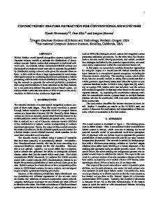
Figure 1. Relationship between raw data distribution and the data transformed to a lower dimensional space using PCA, PPCA, and PFA. Raw dataset in three dimensions (a) are transformed to a two-dimensional feature space using PCA (b), PPCA (c), and PFA (d). The translucent ellipsoid in (a) and ellipses in (b) and (c) represent the 1.96 standard deviations.

Figure 1 shows a pictorial example of a raw dataset in three dimensions transformed to a 2D feature space using PCA, PPCA, and PFA.

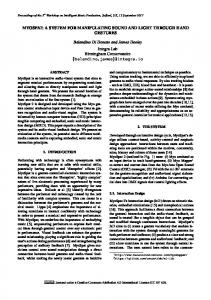
Class-based feature extraction algorithms Global feature reduction algorithms provide a feasible approach for projecting high-dimensional data into a lower dimensional subspace. However, class separability can be reduced during this process. In Figure 2a, for example, when © 2007 CASI

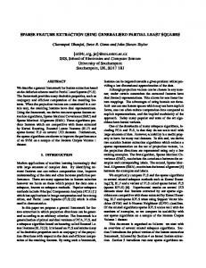
classes 1 and 2 are projected onto the global principal axis by PCA, they cannot be distinguished from one another. Alternatively, if we project classes 1 and 2 onto their own subprincipal axes as in Figure 2b, they can be classified as different clusters. This is the basic principle behind class-based feature reduction algorithms. The class-based version of PCA, PPCA, and PFA (CPCA, CPPCA, and CPFA, respectively) for the classification of hyperspectral imagery is conducted in a two-stage procedure including training and classification as follows (Figure 3): 165

Vol. 33, No. 3, June/juin 2007

Figure 2. Basic principle of class-based feature extraction: (a) global PCA; (b) class-based feature reduction classification.

vector y belonging to each subspace (p1, p2, þ, pn) are calculated according to the normal density function. The decision criteria is y ∈ C i,

i = arg max{p j , j = 1, K n}

(8)

j

The class-based feature reduction algorithm borrows the decision rule from the maximum likelihood algorithm and constrains the feature reduction within each class. Therefore, it decreases the computational burden without seriously compromising the class separability. Actually, the computational complexity for a covariance matrix in a maximum likelihood classifier is O(Nq2), where N represents the total number of training samples (Richards and Jia, 1999). The computational complexity in class-based feature reduction algorithms decreases to O(nN′p2), where n is the class number, and N′ is the sample number of each class. Since p is usually far less than q, and nN′ is approximately equal to N, the computational burden drops to a reasonable level. Figure 3. Class-based feature extraction classification process. C, classifier; P, probability; T, transformation.

Experiments

(1) Collect the training data for n classes C1, þ, Cn. For each class, feature reduction algorithms PCA, PPCA, and PFA are used to calculate the latent subspace. As a result, n low-dimensional Gaussian clusters are found in the hyperspace, and their distribution parameters are estimated. Generally speaking, an n low-dimensional Gaussian distribution can be acquired from the linear projection operators: X1 = T1(Y1), þ, Xn = Tn(Yn), where Tn is the transformation formula, i.e., Equations (1), (3), or (7).

We conducted two simulation experiments to study the characteristics of PPCA, PFA, and the class-based feature extraction algorithms. We then applied class-based feature extraction classifiers to a CASI 2 hyperspectral image to detect and map yellow starthistle in our study area. The results are evaluated and compared with conventional hyperspectral classifiers.

(2) Classification is conducted on a pixel to pixel basis. The spectrum vector of each pixel y in hyperspectral imagery is projected into n latent subspaces through T1–Tn, respectively, and then the likelihoods of each projected

A series of numerical experiments were simulated in MATLAB® to compare the performance of PPCA3 and PFA under controlled circumstances. First, we generated a random

3

Simulation 1: PPCA and PFA

PCA and PPCA principle axes have the same projection directions, so we only use PPCA to compare with PFA.

166

© 2007 CASI

Canadian Journal of Remote Sensing / Journal canadien de télédétection

Figure 4. A comparison between PPCA and PFA: (a) dataset 1 results; (b) dataset 2 results.

variable with a one-dimensional (1D) Gaussian distribution: X ~ N(0, 1). Second, we rotated this dataset 45° in the extended 2D space. Third, two random noise variables with a 1D Gaussian distribution n1 ~ N(0, Ψ1), n2 ~ N(0, Ψ2) along the y1 and y2 directions were added to X. In the first dataset, Ψ1 = Ψ2 = 0.01, and in the second dataset, Ψ1 = 0.25 and Ψ2 = 0.01. As a result, two new random variables Y1 and Y2 were generated in R2. We acquired their principal axes while running the PPCA and PFA algorithms to reduce the 2D data to 1D. In dataset 1, the PPCA principal axis and PFA principal axis (the first column vector of transform matrix ⌳) were both close to the 45° line (Figure 4a). Furthermore, the variances of n1 and n2 were very close to the true values. Results are summarized in Table 1. In Figure 4b, the principle component axis of PPCA is oriented in a direction that explains most of the variance in the data, but it deviates from the original latent data axis. PFA provided a better estimation. The results are summarized in Table 2. Despite the better estimate, there are two important factors to consider with PFA. First, different combinations of initial input parameters produce different results, so it is difficult to interpret results by identifying latent variables. From our experience, it is a good choice to input PPCA results as the initial condition so that EM can converge quickly. The second is simply computational, as PFA always runs much longer than PPCA because the EM is an iterative algorithm. Simulation 2: class-based feature extraction classification In the second simulation, three 2D training classes were generated from a 1D standard Gaussian distribution. The rotation angles and Gaussian noise variances are summarized in Table 3. CPCA, CPPCA, and CPFA were then applied to extract the subspace statistical parameters. In Figure 5, the solid lines represent the true rotation directions, the dash–dot lines are the principle axes of CPCA (or CPPCA), and the dash–dash lines are the CPFA axes. Three hundred test samples were generated for each class using the same set of parameters © 2007 CASI

Table 1. PPCA and PFA results for dataset 1. Principal axis vector

Error structure W

PPCA

[0.7054

0.7088]T

0.0102  0 

0  0.0102 

PFA

[0.7092

0.7126]T

0.0116  0 

0  0.0117

Table 2. PPCA and PFA results for dataset 2. Principal axis vector

Error structure W

PPCA

[ −0.7557

− 0.6549]T

0.1176  0 

PFA

[ −1.0717

− 0.9636 ]T

0  0.1614  0  0.0835  

0  0.1176 

Table 3. Training sample parameters (see Figure 5). Class

No. of samples

Rotation angle (°)

y1 variance

y2 variance

1 2 3

300 300 300

60 5 120

0.09 0.04 0.36

0.36 0.36 0.04

listed in Table 3. CPCA, CPPCA, and CPFA classifiers were applied to this test dataset. From Figures 6b–6d, we find that all three class-based feature extraction algorithms provided satisfactory classification results. These simulations show that the class-based feature extraction algorithms are suitable for low-dimensional datasets. However, some class 3 test samples are misclassified as class 1 (see lower right corners of the plots shown in Figures 6b–6d), although samples are far away from the centroid of class 1. We define this misclassification as shuttle phenomenon (i.e., these samples from different classes being misclassified in the same 167

Vol. 33, No. 3, June/juin 2007

Figure 5. Three graphs of 2D training samples. Dash–dot lines represent true rotation directions, solid lines are the principal axes of CPCA–CPPCA, and dash–dash lines are the CPFA principal axes. CPFA principal axes almost overlap the CPCA–CPPCA principal axes. +, group 1 training samples; ×, group 2 training samples; 䉭, group 3 training samples.

class when using class-based feature extraction methods). Shuttle phenomenon is not surprising, since the probabilities of those samples in class 1 are larger than those in class 3 after projection. Generally speaking, distances measured in highdimensional space are invalid after projecting in lower dimensional subspaces. If the principle axes of two classes are parallel, and the straight line through their centroids is perpendicular to the principle axes, the shuttle phenomenon will be rather obvious. However, this restriction should not seriously undermine the class-based feature extraction algorithms, since these conditions are not critical, especially in the hyperspectral space. We can avoid the shuttle phenomenon by increasing the dimensions of the class subspaces. CASI 2 land cover supervised classification The CASI 2 is a charge-coupled device (CCD) push-broom imager designed for the acquisition of visible and near-infrared hyperspectral imagery. It has 48 channels covering the wavelengths ranging from 0.43 to 0.97 µm (blue to nearinfrared). The CASI 2 image used in this paper was acquired over Bear Creek, Yolo County, California, on 30 June 2002 with a spatial resolution of 2 m. The CASI 2 image was georegistered to a digital orthophoto quarter quadrangles (1 m US Geological Survey DOQQ) base map using the first-order polynomial method. The average root-mean-squared error 168

(RMSerror) of the georegistration was around 2 m when using 10 ground-control points (GCPs). The brightness value of the rectified image was resampled using a nearest-neighbor algorithm. A 400 × 400 pixel image was cropped from the whole scene and used in this study (Figure 7). Since only a single date of hyperspectral image was used for classification and the training data were not extended through space and (or) time, we did not perform atmosphere correction (Song et al., 2001). Yellow starthistle (YST), which was recognized as the worst invasive weed in California (DiTomaso, 2000), is mainly distributed between the creek and Highway 16 (Miao et al., 2006). It blossoms yellow flowers during the summer and shows as a light yellow hue in the false color image (Figure 7). The riparian plant salt cedar is found mainly along the creek. Five other land cover classes seen in the CASI image (Figure 7) are water, highway, native trees (oak), mountain area, and bare ground. A field trip was conducted in July 2002 to verify the sample pixels selected for supervised classification. The spectral signatures of these seven classes are shown in Figure 8. Digital numbers (DN) were not converted to the reflectance through radiometric correction. The CASI 2 image was used to illustrate the performances of class-based feature extraction algorithms for hyperspectral classification. The results are also compared with other common hyperspectral classifiers.

© 2007 CASI

Canadian Journal of Remote Sensing / Journal canadien de télédétection

Figure 6. Comparing CPCA, CPPCA, and CPFA classification performance (+, class 1; ×, class 2; 䉭, class 3): (a) test samples; (b) CPCA; (c) CPPCA; (d) CPFA.

The kappa coefficient, k, is an index of classification accuracy derived from the following error matrix:

k=

N ∑ x kk − ∑ x k + x + k k

k

N 2 − ∑ xk + x+ k

(9)

k

where xij represents the elements of the error matrix (Richards and Jia, 1999). The kappa coefficient is commonly used in remote sensing analysis as a measure of map accuracy, since it indirectly incorporates the omission and commission errors of an error matrix (Congalton, 1991). One of the advantages of using the kappa coefficient is that it allows the statistical comparison between two classified maps. Therefore, we used the kappa coefficient to estimate and compare the classification accuracies of all classifiers in this research: class-based feature extraction; a band selection scheme based on maximum

© 2007 CASI

Bhattacharyya distance; and three global feature extraction approaches, namely PCA, LDA, and SPCT. We selected 4, 6, 8, 10, 12, and 48 bands based on maximum Bhattacharyya distance criteria and input them to a maximum likelihood classifier (MLC) (Richards and Jia 1999). Bhattacharyya distance (B distance) is a pairwise measure of class separability (Kailath 1967): −1

Bij =

(mi − mj ) T  ⌺i + ⌺j   (mi − mj )  8  2    (⌺i + ⌺j )/ 2  + ln  2 1 1   2 2 ⌺ ⌺ j  i 

(10)

where ⌺i is the class covariance matrix, and mi is the class mean vector. The average value of all possible class pairs was used to select the bands with maximum between-class separability.

169

Vol. 33, No. 3, June/juin 2007

Figure 7. CASI 2 false color image used in this study (red = 850.0 ± 5.9 nm; green = 653.7 ± 5.9 nm; blue = 551.0 ± 5.8 nm).

Figure 8. Spectral signatures of seven land classes derived from the CASI 2 image. Digital numbers (DN) were not converted to the reflectance, since only a single date of hyperspectral image was used for classification. YST, yellow starthistle.

170

© 2007 CASI

Canadian Journal of Remote Sensing / Journal canadien de télédétection

Figure 9. Logarithm of eigenvalues of each class.

Equal priors were assumed for MLC. Although it is a simple band selection scheme, it is a good starting point to establish a baseline to compare other feature extraction classifiers. The first three, five, seven, and nine features with maximum eigenvalues, which represented the maximum data variance when projecting the hyperspectral data on the corresponding principal axes, were selected from each class from CPCA, CPPCA, and CPFA classifiers, respectively. Similarly, the first three, five, seven, and nine features were also selected from the global PCA classifier. The first two, four, and six discriminant variables (features) were selected from the LDA classifier. As for the SPCT classifier, principal components 1, 2, and 3 (PC1, PC2, and PC3) were selected from subgroup 1 (bands 1–26, 0.43–0.70 µm) and subgroup 2 (bands 27–48, 0.71–0.97 µm). The critical decision in class-based feature extraction algorithms is determining how many axes to choose when projecting the hyperspectral image into subspaces. More features augments class separability but requires more training samples and hampers computational efficiency (Burnham and Anderson, 2002). In addition, by keeping more features, the classifiers will be more complex and classification accuracy will decrease, given the limited training sample size (Burnham and Anderson, 2002). Analysis of eigenvalues was used to explore data dimensionality and the number of features to select. Although each class could be defined by a different number of features, they were assumed to be the same in this research to illustrate the effect of the increasing number of features on classifiers. Eigenvalues were calculated for each class, ranked in decreasing order (Figure 9). The accumulated © 2007 CASI

Table 4. Accumulated ratios of the first three eigenvalues (%). Class

Eigenvalue (%)

Water (W) Yellow starthistle (YST) Highway (HW) Salt cedar (SC) Native tree (NT) Mountain area (MT) Bare ground (BG)

97.64 98.10 90.86 98.56 97.61 99.05 98.53

ratios of the first three eigenvalues to the total variance for each class are summarized in Table 4, which indicates that the first three eigenvectors can explain the majority of the variance for each class. This fact confirmed that most of the data variance was stored in a latent subspace, and the minimal dimension of the subspace was three. We ran every algorithm 20 times. During each round of classification, we randomly selected 150 training samples from the class sample pool without replacement. The remaining samples were used to estimate the classification accuracy. The number of samples used in the classification experiments is summarized in Table 5. This Monte-Carlo approach to classification produces a more robust estimate of the kappa coefficient and thus a better evaluation of the true performance of each classification algorithm. The kappa coefficients for all classifiers are illustrated by box plots in Figure 10. Each box and whisker plot provides a 171

Vol. 33, No. 3, June/juin 2007 Table 5. Number of samples for the seven classes.

Table 6. Error matrix of the CPCA classification with seven features (k = 0.946, overall accuracy = 95.4%).

Class

No. of training samples

No. of test samples

Total

Yellow star-thistle (YST) Bare ground (BG) Salt cedar (SC) Native tree (NT) Mountain area (MT) Highway (HW) Water (W) Total

150 150 150 150 150 150 150 1050

301 250 256 177 269 177 118 1548

451 400 406 327 419 327 268 2598

Note: Training and test samples were randomly selected from the class sample pool, which was visually selected in Figure 7 and verified by ground reference data.

five-number summary (the smallest observation, lower quartile, median, upper quartile, and largest observation) of the 20 kappa coefficients for each classifier. To show the changing trend as a function of the number of bands or features used in the classification, we connected the median kappa coefficient for each classification. The kappa accuracies of the band selection classifier (BS in Figure 10) reached a peak of about 0.925 when retaining eight bands, and the CPCA classifier requires only the first seven features to reach a peak of 0.946. Although CPPCA and CPFA were more appealing theoretically, their classification performances were not satisfactory, and their highest kappa coefficients were only

Reference class Map class

YST

BG

SC

NT

MT

HW

W

Total

YST BG SC NT MT HW W Total

281 20 0 0 0 0 0 301

15 235 0 0 0 0 0 250

0 0 249 7 0 0 0 256

0 0 4 173 0 0 0 177

17 2 0 3 247 0 0 269

0 0 0 0 1 176 0 177

0 0 1 1 0 0 116 118

313 257 254 184 248 176 116 1548

Note: Class abbreviations as in Tables 4 and 5.

about 0.896 and 0.836, respectively. The global PCA classifier with five and seven features worked well, and the kappa coefficient was as high as 0.923, better than the LDA approaches, which peaked at 0.905 with six features. SPCT with six features had a good performance with a kappa coefficient of 0.931. In summary, CPCA had the best performance for supervised classification of CASI hyperspectral data in this study. Although CPPCA and CPFA performed well using the simulated data, they did not provide satisfactory results for classification of the hyperspectral data due primarily to the limited number of training samples. As the CPCA method

Figure 10. Box plots of kappa coefficients for each classification algorithm. From left to right: CPCA with 3, 5, 7, and 9 features; CPPCA with 3, 5, 7, and 9 features; CPFA with 3, 5, 7, and 9 features; Bhattacharyya band selection (BS) with 4, 6, 8, 10, 12, and 48 bands; PCA with 3, 5, and 7 features; LDA with first 3, 4, 5, and 6 discriminant features; and SPCT with 6 features. Each plot gives the smallest observation, lower quartile, median, upper quartile, and largest observation. 172

© 2007 CASI

Canadian Journal of Remote Sensing / Journal canadien de télédétection

resulted in the “best” classification, the error matrix of the CPCA classifier with seven features is illustrated in Table 6. The left column represents the thematic map classes, and the top row represents the ground truth or reference classes. The CPCA-classified map derived using the first seven features is shown in Figure 11.

Discussion and conclusion Hyperspectral remote sensing images due to extremely high spectral resolution have strong correlations between various band ranges. This property results in flat class clusters (i.e., “Gaussian pancakes”) in hyperspectral space (Brunzell and Eriksson, 2000). In addition, Jimenez and Landgrebe (1998) pointed out that hyperspace is almost empty for highly correlated hyperspectral data, and low-dimensional linear projections of high-dimensional datasets tend to be normally distributed or a combination of normal distributions. The first observation results in the concentration of most of the hyperspectral data in specific latent subspaces, and the second observation supports the Gaussian distribution assumption required by the maximum likelihood classification algorithm used in this paper. Therefore, class-based subspaces can be modelled as “Gaussian pancakes floating in sparse hyperspace.” This paper evaluated and compared three class-based feature extraction algorithms for classification of hyperspectral imagery. Each land cover class was projected onto a low-dimensional subspace using class-based principal components analysis (CPCA), class-based probabilistic principal components analysis

(CPPCA), and class-based probabilistic factor analysis (CPFA). Supervised classification (maximum likelihood classifier or MLC) of several land classes was conducted in a two-stage process: the training data were used to determine the low-dimensional latent subspace for each class, and then every pixel of the hyperspectral image was projected onto the latent spaces and its class membership was determined with an MLC. Although a normal data distribution is a requirement of the MLC, many researchers have found that MLC performs well even on data that are not normally distributed. Hastie et al. (2001) found that the most likely reason was that the data could only support simple decision boundaries defined by linear or quadratic functions, and the estimates provided by the Gaussian models were stable. Thus the assumption of a normal distribution for MLC was relaxed in this paper. Two problems remain for class-based feature extraction classifiers. The first is an appropriate method for selecting the suitable number of features. In Figure 10, we find that every algorithm (except LCA and SPCT) has a peak kappa coefficient, which represents the optimal number of features given a limited training sample size known as the Hughes phenomenon (Landgrebe, 2002). We recommend choosing the feature number around the peak kappa value to achieve maximum classification accuracy. However, it is still problematic to derive a criterion to determine the optimum number of features for each class without conducting laborious experiments. The second problem is the shuttle phenomenon described in simulation 2. It is a shortcoming of class-based feature extraction classifiers, especially for a low-dimensional

Figure 11. Class-based PCA classification map. © 2007 CASI

173

Vol. 33, No. 3, June/juin 2007

dataset. This phenomenon can be avoided by increasing the number of features. For example, the shuttle phenomenon would not occur if two features remained in each 2D class cluster in Figures 6b–6d. On the other hand, increasing the number of features may lead to the Hughes phenomenon. Therefore, the proper number of features should be selected to balance this trade-off. In this study, based on eigen-analysis, we increased the number of features starting from three. The CPFA is a plausible choice theoretically for data reduction or feature extraction. The simulation experiments verified its effectiveness for the classification of 2D data. However, the CASI 2 experiment demonstrated that the CPFA feature extraction did not provide accurate classification of land classes on hyperspectral imagery because the increasing complexity of the classifier cannot be supported by a limited amount of training samples. Furthermore, CPFA ran much slower than other class-based feature extraction algorithms, since it uses the iterative EM algorithm. Although CPPCA and CPCA shared the same latent subspaces, the CPCA feature extraction resulted in a number of features that resulted in a more accurate land classification. We believe the reasons for this are as follows: (i) CPCA is more robust for datasets that are not normally distributed compared with CPPCA, which requires strict assumptions of normality; and (ii) CPPCA results in lower separability between classes, since it reduced the cluster distribution (Figure 1). In conclusion, CPCA is recommended as the best class-based feature extraction method for hyperspectral image classification. CPCA is a flexible and effective feature extraction method for producing a set of features that produce a reasonable tradeoff between classification accuracy and computation efficiency for hyperspectral image classification. However, a few problems remain. First of all, since the features that result from this transformation are a linear mixture of all hyperspectral input bands, interpretability is sacrificed when conducting CPCA. Another problem concerns the separability of classes. If the separability of two classes depends only on a few spectral bands, and the variances of these diagnostic bands are relatively small, as in some mineral remote sensing applications, CPCA would likely ignore the difference between the two classes. Our future work will involve the incorporation of conventional feature extraction or classification methods such as segmented principal components transformation (SPCT) and spectral angle mapper (SAM) into the class-based framework to circumvent these difficulties.

References Bartholomew, D.J. 1987. Latent variable models and factor analysis. Oxford University Press, New York. Basilevsky, A. 1994. Statistical factor analysis and related methods: theory and applications. Wiley, New York. Brunzell, H., and Eriksson, J. 2000. Feature reduction for classification of multidimensional data. Pattern Recognition, Vol. 33, pp. 1741–1748.

Burnham, K.P., and Anderson, D.R. 2002. Model selection and multimodel inference: a practical information–theoretic approach. Springer, New York. Chang, C.I., Du, Q., Sun, T.L., and Althouse, M.L.G. 1999. A joint band prioritization and band-decorrelation approach to band selection for hyperspectral image classification. IEEE Transactions on Geoscience and Remote Sensing, Vol. 37, pp. 2631–2641. Congalton, R.G. 1991. A review of assessing the accuracy of classifications of remotely sensed data. Remote Sensing of Environment, Vol. 37, pp. 35–46. Cooper, J.C.B. 1983. Factor-analysis — an overview. American Statistician, Vol. 37, pp. 141–147. DiTomaso, J.M. 2000. Invasive weeds in rangelands: species, impacts, and management. Weed Science, Vol. 48, pp. 255–265. Hastie, T., Tibshirani, R., and Friedman, J.H. 2001. The elements of statistical learning: data mining, inference, and prediction. Springer, New York. Jia, X., and Richards, J.A. 1999. Segmented principal components transformation for efficient hyperspectral remote-sensing image display and classification. IEEE Transactions on Geoscience and Remote Sensing, Vol. 37, pp. 538–542. Jimenez, L.O., and Landgrebe, D.A. 1998. Supervised classification in highdimensional space: geometrical, statistical, and asymptotical properties of multivariate data. IEEE Transactions on Systems, Man, and Cybernetics: Part C — Applications and Reviews, Vol. 28, pp. 39–54. Jimenez, L.O., and Landgrebe, D.A. 1999. Hyperspectral data analysis and supervised feature reduction via projection pursuit. IEEE Transactions on Geoscience and Remote Sensing, Vol. 37, pp. 2653–2667. Jolliffe, I.T. 1986. Principal component analysis. Springer-Verlag, New York. Kailath, T. 1967. Divergence and Bhattacharyya distance measures in signal selection. IEEE Transactions on Communication Technology, Vol. 15, No. 1, pp. 52–60. Kambhatla, N., and Leen, T.K. 1997. Dimension reduction by local principal component analysis. Neural Computation, Vol. 9, pp. 1493–1516. Kumar, S., Ghosh, J., and Crawford, M.M. 2001. Best-bases feature extraction algorithms for classification of hyperspectral data. IEEE Transactions on Geoscience and Remote Sensing, Vol. 39, pp. 1368–1379. Landgrebe, D. 2002. Hyperspectral image data analysis. IEEE Signal Processing Magazine, Vol. 19, pp. 17–28. Landgrebe, D.A., Serpico, S.B., Crawford, M.M., and Singhroy, V. 2001. Introduction to the special issue on analysis of hyperspectral image data. IEEE Transactions on Geoscience and Remote Sensing, Vol. 39, pp. 1343–1345. Marchette, D.J., and Poston, W.L. 1999. Local dimensionality reduction. Computational Statistics, Vol. 14, pp. 469–489. Mausel, P.W., Kramber, W.J., and Lee, J.K. 1990. Optimum band selection for supervised classification of multispectral data. Photogrammetric Engineering and Remote Sensing, Vol. 56, pp. 55–60. Miao, X., Gong, P., Swope, S., Pu, R., Carruthers, R., Anderson, G.L., Heaton, J.S., and Tracy, C.R. 2006. Estimation of yellow starthistle abundance through CASI-2 hyperspectral imagery using linear spectral mixture models. Remote Sensing of Environment, Vol. 101, pp. 329–341. Richards, J.A., and Jia, X. 1999. Remote sensing digital image analysis: an introduction. 3rd ed. Springer-Verlag, New York. Rubin, D.B., and Thayer, D.T. 1982. Em algorithms for ML factor-analysis. Psychometrika, Vol. 47, pp. 69–76.

174

© 2007 CASI

Canadian Journal of Remote Sensing / Journal canadien de télédétection Song, C., Woodcock, C.E., Soto, K.C., Lenney, M.P., and Macomber, S.A. 2001. Classification and change detection using Landsat TM data: when and how to correct atmospheric effects? Remote Sensing of Environment, Vol. 75, pp. 230–244. Stone, C.J. 1995. A course in probability and statistics. Duxbury Press, Pacific Grove, Calif. Tipping, M.E., and Bishop, C.M. 1999a. Mixtures of probabilistic principal component analyzers. Neural Computation, Vol. 11, pp. 443–482. Tipping, M.E., and Bishop, C.M. 1999b. Probabilistic principal component analysis. Journal of the Royal Statistical Society, Series B — Statistical Methodology, Vol. 61, pp. 611–622. Webb, A. 2002. Statistical pattern recognition. John Wiley & Sons, West Sussex, UK. Yu, B., Ostland, I.M., Gong, P., and Pu, R.L. 1999. Penalized discriminant analysis of in situ hyperspectral data for conifer species recognition. IEEE Transactions on Geoscience and Remote Sensing, Vol. 37, pp. 2569–2577.

List of abbreviations CPCA

class-based principal components analysis

CPFA

class-based probabilistic factor analysis

CPPCA

class-based probabilistic principal components analysis

LDA

linear discriminant analysis

PCA

principal components analysis

PFA

probabilistic factor analysis

PPCA

probabilistic principal components analysis

SPCT

segmented principal components transformation

© 2007 CASI

175