Applying Constraint Programming to Rigid Body Protein ... - CiteSeerX

Applying Constraint Programming to Rigid Body Protein Docking Ludwig Krippahl and Pedro Barahona Dep. de Informática, Universidade Nova de Lisboa, 2825 Monte de Caparica, Portugal [email protected], [email protected]

Abstract. In this paper we show how Constraint Programming (CP) techniques can improve the efficiency and applicability of grid-based algorithms for optimising surface contact between complex solids. We use BiGGER [1] (Bimolecular complex Generation with Global Evaluation and Ranking) to illustrate the method as applied to modelling protein interactions, an important effort in current bioinformatics. BiGGER prunes the search space by maintaining bounds consistency on interval constraints that model the requirement for the shapes to be in contact but not overlapping, and by using a branch and bound approach to search the models with the best fit. This CP approach gives BiGGER some efficiency advantages over popular protein docking methods that use Fourier transforms to match protein structures. We also present an efficient algorithm to actively impose a broad range of constraints or combinations of constraints on distances between points of the two structures to dock, which allows the use of experimental data to increase the effectiveness and speed of modelling protein interactions and which cannot be done as efficiently in Fourier transform methods. This shows that constraint programming provides a different approach to protein docking (and fitting of shapes in general) that increases the scope of application while improving efficiency.

1. Introduction The general problem we address in this paper is to fit two solids of arbitrary shape so as to maximize the surface of contact. This problem is important in bioinformatics for modelling protein interactions, also known as protein docking. Protein interactions play a crucial role in all biological systems, and knowing the structure of a protein complex is an essential step in understanding the interaction mechanism. In this paper we will focus on the particular case of protein docking, currently the area of greater application of these algorithms, but the results are general and applicable to calculating configurations of maximal contact for solids of arbitrary shape. The most important aspects of this paper are the efficiency gained by using constraint propagation techniques, which puts our method on the same level of efficiency as other current approaches, and the propagation of distance constraints between sets of points in the two structures. The latter is of especial importance because the algorithm we present allows the pruning of the search space using

partially ambiguous or uncertain data, and is thus applicable to a wide range of realworld situations. Modelling software provides useful tools to help researchers elucidate protein interaction mechanisms, and two decades since the pioneering work of Katzir and others [2] have seen significant developments in algorithms to generate models and scoring functions to select the most likely candidates. The diversity of current approaches is evident in the CAPRI (Critical Assessment of PRediction of Interactions) experiment [3]. A common trend is to model interactions using only knowledge derived from the structure and physicochemical properties of the proteins involved. Some algorithms have been developed [1, 4, 5] or adapted [6] to use data on the interaction mechanisms, but this approach is still the exception rather than the norm. BiGGER is one of these exceptions [1, 4], and it has been developed from inception to help the researcher bring into the modelling process as much data as available. Previous results show that BiGGER can be a powerful modelling tool when used in this manner, even when the experimental data are only applied after the search stage to score the models produced [1, 4, 7, 8, 9, 10, 11]. Of all protein docking approaches, the most popular is to generate a threedimensional matrix encoding the shape of each solid, and then match the two matrices by calculating a correlation matrix. This approach was first reported by KatchalskiKatzir [2], and relied on Fast Fourier Transform method (FFT) to generate the correlation matrix. Some current implementations of this algorithm to protein interaction modelling are MolFit [2], ZDOCK [12], FTDock [6], DOT [13], and GRAMM [14]. Our implementation, BiGGER, uses a search in real (geometrical) space instead of Fourier transforms to fit two solids of arbitrary shape. BiGGER and Chemera, the graphical interface, form a tool to study protein-protein interaction that is publicly available and can be downloaded from http://www.cqfb.fct.unl.pt/bioin/chemera/ In this paper we show that an algorithm that actively enforces the constraints inherent to the docking problem virtually eliminates the time advantage of the FFT approach, is in practice often significantly faster, and results in a hundred-fold reduction in memory requirements. Furthermore, this approach can be naturally adapted to additionally constrained searches using experimental data that are not efficiently accommodated with the FFT techniques. The paper is organised as follows. In section 2 we elaborate on the docking problem and the grid method for fitting together two arbitrary shapes. Section 3 explains the BiGGER search algorithm and how constraints are enforced to improve efficiency. Section 4 shows the performance results, and the conclusions follow in section 5.

2 The Docking Problem At the core of this approach to matching of irregular structures are the grid and the measure of surface contact. The grid is a very straightforward representation using a regular cubic lattice of cells, where each cell can be either an empty cell, a surface

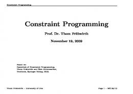
cell, or a core cell. The surface cells define the surface of the structure, and the overlap of surface cells measures the surface of contact. Figure 1 illustrates these concepts, showing on the first two panels a cutaway diagram of the grid representing a protein structure, and on the third panel a cutaway diagram of two grids in contact, showing the contact region corresponding to a set of overlapping surface cells.

Fig. 1. The image on the left shows a protein structure overlaid on a cutaway of the respective grid, with grey spheres representing the atoms of the protein. The centre figure shows only the grid, cut to show the surface in grey and the core region in white. The rightmost image shows the contact between two grids as a black line of grid cells at the interface.

This approach is especially useful for molecular modelling because intermolecular contacts are not crisp like they appear to be at a macroscopic scale, but rather diffuse and a function of electrostatic repulsions between the atoms. The grid can model this feature quite naturally by adjusting the thickness of the surface region and its placement relative to the structure to be modelled. Closer inspection of the first panel on Figure 1 reveals that the surface cells lie outside the Van der Waals surfaces of the atoms (white spheres on the first panel). When these surface cells overlap with those of another grid, the placement of the grids corresponds to a small separation of the Van der Waals surfaces on the protein complex, which is more realistic than actual contact. The placement of the surface region can be modified according to the nature of the objects and contacts that are being modelled, from rigid macroscopic objects to diffuse electron clouds in atoms, so this is a general approach that can cover a wide range of applications. The core cells mark the forbidden overlaps; overlapping core cells indicate that parts of the two structures are occupying the same space and this configuration is disallowed. Overlap between core and surface cells can be ignored because in our model the surface region corresponds to a layer external to the structure, as explained above. 2.1 Protein docking and the Fast Fourier Transform approach. Given these definitions of allowed configurations and of how to measure surface contact, one can search all configurations by moving one grid relative to the other and examining the overlapping cells of the two grids. This translation search must be repeated for each orientation of one partner relative to the other, in order to search the rotation space as well. Typically, the rotational space is sampled in steps of 15º around each of the three orthogonal axes of rotation, for a total of approximately six thousand orientations.

For each relative orientation, the naïve algorithm examines N3 different configurations, where N is the width of the grid, and for each configuration O(N3) cells, for a time complexity of O(N6). Currently the most used algorithm in protein docking is the grid method using Fast Fourier Transform (FFT), in which the grids are three-dimensional matrices, and the surface overlap is measured by the correlation matrix calculated from the two matrices representing the two proteins. The FFT algorithm allows the correlation matrix to be calculated quickly as a matrix multiplication of the Fourier transforms of the two matrices to correlate. This computation has a time complexity of O(N3Log(N)), which clearly outperforms the O(N6)) time complexity of the translational search of the naïve search described above, thus justifying the popularity of the FFT approach. Again, as in all grid-based docking approaches, one grid must be generated for each orientation of one of the partners relative to the other, and whether in BiGGER, the FFT approach, or in the naïve approach, this translational search must be repeated for every orientation, typically thousands of times. Because of the efficiency of FFT, protein docking using grid algorithms with a real (geometrical) space search (instead of using Fourier transforms) were not competitive. However we discuss below how constraint programming techniques improve such search, overcome this basic disadvantage, and even give some advantages in computation time, memory requirements and, especially, in the efficient use of information about the interaction, as shown by the results obtained with BiGGER. 2.2 Using data on contacts and distances In some cases there is information about distances between points in the structures, information that can be used to restrict the search region. If this information is a conjunction of distance limits, then it is trivial to restrict the search to the volumes allowed by all the distances. However, real applications may be more complex. For modelling protein interactions, it is often the case that one can obtain data on important residues or atoms from such techniques as site directed mutagenesis or NMR titrations, or even from theoretical considerations, but it is rare to be absolutely certain of these data. The most common situation is to have a set of likely distance constraints of which not all necessarily hold. Typically, we would like to impose a constraint of the form: At least K atoms of set A must be within R of at least one atom of set B

(1)

where set A is on one protein and set B on the other, and R a distance value. This constraint results in combinatorial problem with a large number of disjunctions, since the distances need only hold for at least one of any combination of K elements of A. The FFT approach is especially unsuited for taking advantage of this type of information, since one cannot use this technique to find the correlation only of parts of all possible configurations of the two grids. With FFT the only way to use constraints is after the search, in a passive generate and test approach, validating or rejecting candidate configurations after the search. Validating each configuration according to constraint (1) is simple, and any docking algorithm can do this. BiGGER itself has been used in this way with considerable success. Chemera, the application

that accompanies BiGGER in our distribution of this software package, allows the user to score the models produced by BiGGER according to inter-atomic distances. Some examples of this approach using BiGGER are in electron transfer complexes [7, 8, 9] or in modelling complexes using NMR and site-directed mutagenesis data [10, 11]. But the best way to use this information is as active constraints, pruning the search space to improve computation time, and in Section 3.4 we show that the combination of grid representations and real (geometrical) space search is particularly suited to enforcing this global constraint due to the structure of the nested loops for the search in the X, Y, and Z directions. Though we discuss this geometry constraints problem as it presents itself in protein docking, this is a general problem. These distance values may be from uncertain NMR data, but they may also be from alternative positions for mooring lines, a lower limit for the number of bolts to secure two parts, or any other case where there are more alternatives to distance limits between points in the two structures than those limits that must be enforced.

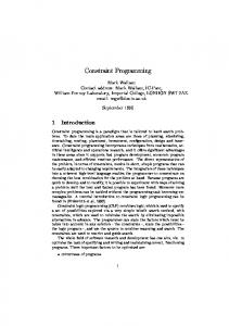
3. Method The basic method of searching through the translation space for the configurations with the largest surface contact is simple and straightforward. This section focuses on the modifications that make this method much more efficient than the O(N6) time complexity of the basic approach. Two constraints contribute to this efficiency, when adequately enforced: a) restricting the search to positions where surface regions overlap, and b) eliminating positions where core regions overlap. In addition, restricting the search to those regions where it is possible to have a greater surface contact than that of the worst solution to be kept can improve efficiency in some cases, but this last constraint is not useful in general, and is only discussed briefly. Finally, we show how the additional constraint (1) discussed above, can be efficiently implemented in this algorithm and further decrease computation time when the relevant information is available. 3.1 Restricting the search to surface overlapping regions. A significant proportion of all possible configurations for the two grids results in no surface overlap. Much can be gained by restricting the search to those configurations where surface cells of one grid overlap surface cells of the other. This is achieved by encoding the grids in a convenient way: instead of individual cells, grids are composed of lists of intervals specifying the segments of similar cells along the X coordinate. These lists are arranged in a two-dimensional array on the Y-Z plane. Figure 2 illustrates this encoding process for two lines, along the horizontal axis, on an X-Y plane where Z = j. The line on the top contains only surface cells, and is encoded as two surface segments, from X coordinates 3 through 7 and 12 through 18. This line in the grid is thus encoded as a list of two intervals Sij = [(3;7), (12;18)] where i is the Y coordinate. The other line in this example contains both surface and

core cells, and is encoded as two lists: a list of surface cells Skj = [(2;3), (7;9), (20;21)] and a list of core cells Ckj = [(4;6), (10;20)]. Y i

Sij = [(3;7), (12;18)]

k

Skj = [(2;3), (7;9), (20;21)] Ckj = [(4;6), (10;20)]

1

5

10

15

20

X

Fig. 2. This figure illustrates the encoding of the grid as segments, with each segment containing only the X coordinates of the start and end points of a row of consecutive grid cells of the same type. Surface grids are represented in light grey and surface segments in black, core grids in dark grey and core segments in white.

This encoding not only reduces the memory requirements for storing the grids, but also leads naturally to searching along the X axis by comparing segments instead of by running through all the possible displacements along this coordinate. Given two surface segments, one from each structure and aligned in the same Y and Z coordinates, we can calculate the displacements where overlap will occur simply from the X coordinates of the extremities of the segments. Representing by variable x the displacement of one structure relative to the other along the X direction, this approach of comparing segments efficiently enforces the constraint requiring surface overlaps by reducing the domain of the variable, to only those values where the constraint is verified, as we explain in the next section. 3.2 Eliminating regions of core overlap Another important constraint in this problem is that the core regions of the grids cannot overlap, for that indicates the structures are occupying the same space instead of being in contact. By identifying the configurations where such overlaps occur, it is possible to eliminate from consideration those surface segments on each structure that cannot overlap surface segments on the other structure without violating the core overlap constraint. Some surface segments can thus be discarded from each search along the X axis. Figure 3 illustrates this procedure. One structure, labelled A, is shown in the centre of the image. The other structure, labelled B, will be moved along the horizontal direction to scan all possible configurations but, from the overlap of core segments, a set of positions along the horizontal direction can be eliminated. Structure B is shown in position 1 to the right of A and in position 39 to the left of A, but, in this case, it cannot occupy positions in the centre.

Discarded Segments

A B

1

3 2

2 1

Allowed

L1

B

1

L5

3

5

30

Pruned

39

Allowed

Fig. 3. Grid B is translated along the horizontal direction relative to grid A. The vertical arrows marked 1 indicate the position of B on the lower horizontal bar, which shows the allowed and forbidden values for the position of B. The arrows marked 2 and 3 show the allowed displacement of B. The group of horizontal arrows indicates segments to be discarded.

The domain of variable x (introduced in the previous section to represent the displacement of one structure relative to the other along the X direction) can be pruned from the values 5 to 30. This is a contiguous interval in this example, but the domain of x can be an arbitrary set of intervals in the general case. This domain reduction due to the core overlap constraint propagates to the surface overlap, since some surface segments of A and B will not overlap in valid configurations. Some of these are shown in Figure 3 by the group of arrows to the left of structure A (Discarded Segments, Figure 3). For the last double arrow, for example, the surface cells of structures A and B would only overlap for x=7, a value pruned from the domain of x. In contrast, in the line below such overlap occurs for x = 3, a value kept in the domain. The top three arrows point to surface segments on structure A which can be ignored in this case. The top three surface segments on structure B cannot be ignored because they may overlap with the surface segments of A on the other side, once B is moved to the right of A, but the following four arrows indicate that both the segments to the left of A and those to the right of B can be ignored. Thus the core overlap constraint allows us to reduce the number of surface segments to consider when counting surface overlaps. Figure 4 outlines the algorithm for the translational search. Three variables, z, y, and x, and their respective domains, Dz, Dy, and Dx, represent the translation of B with respect to A. The domains are initialised to include all translations that may result in contacts by a bounds consistency check: if MaxA/MaxB and MinA/MinB are the maximum/minimum coordinate values along the Z axis for the surface grid cells of the two structures, Dz is initialised to [(MinA-MaxB; MaxB-MinA)] (line 1). The same procedure applies to Dy and Dx (lines 3 and 5), but only considering the parts of the structure that can overlap (Dy depends on the value of z, Dx depends on the values of z and y). We shall see in the next sections that these domains can be further pruned by other constraints on the minimum overlap score (section 3.3) and distances between points in the two structures (Section 3.4), so Dz, Dy, and Dx are not necessarily single intervals but sets of intervals. This pruning (Sections 3.3 and 3.4) occurs at the initialisation of the domains (lines 1, 3, and 5).

For each z and y translation value, Dx is initialized (line 5), and the list CoreSets (line 6) is generated, containing the matching sets of core grid segments for the two structures. Grid segment sets are matching when they are aligned by the z, y translation of the B structure, so each entry on this list corresponds to a location in the Z,Y plane and contains the core segments of both structures that are aligned at that location by translating the B structure by the z, y values. Figure 3 shows two such sets, marked L1 and L5, which would be respectively the first and fifth entries of the list of matching core grid segments. L1 contains one core grid segment from A and one from B, L5 contains two core grid segments from A and one from B. 1. Dz ← Z_Translations 2. for each z ∈ Dz do 3. Dy ← Y_Translations(z) 4. for each y ∈ Dy do 5. Dx ← X_Translations(z,y) 6. CoreSets ← Matching_Core_Segs(z,y,Dy) 7. Dx ← RemoveCoreOverlaps(Dy) 8. SurfSets ← Matching_Surf_Segs(z,y,X) 9. CountContacts(XT,SurfacePairs) Fig. 4. Outline of the BiGGER translation search algorithm. The translation search must be repeated for each relative orientation of the two partners.

The BiGGER algorithm then (line 7) imposes bounds consistency on these sets of core grids segments, comparing the bounds of each segment in one structure with the bounds of all matching segments in the other structure for this z, y displacement. If MaxA, MaxB, MinA, and MinB are respectively the upper and lower bounds in the x coordinate for a pair of matching core segments, the algorithm removes the interval (MinA-MaxB; MaxA-MinB) from Dx. Maintaining such bounds consistency requires O(k2) operations, where k is the number of intervals defined by the core grid segments for each line and for each structure. In line 8 the list of matching surface segments is generated, in a similar manner. Note that both the matching core and the surface segments lists take into account Dx, including only those segments that could overlap given this domain (again, by imposing bounds consistency on the intervals). Also, the list of matching surface segments uses Dx already pruned by ruling out the forbidden overlaps (line 7). Finally, the overlap of surface cells is determined for each allowed translation value in Dx. This requires testing the bounds of the matching surface segments in a way similar to imposing bounds consistency, which is of O(k2) for each line, and then counting the contacts along X, which is of O(N). The algorithm performs O(N2) steps by looping through the Dz and Dy (lines 2 and 4), and in each of these steps it loops through the Z,Y plane twice to find the matching core and surface segments (lines 6 and 8) and compare the segment bounds. So each step in the z, y loop is O(N2k2), where k is the number of segments per line (the counting step in line 9 is O(N) and can be ignored). Except for fractal structures, k is a small constant. For convex shapes, for example, k is always two or less, and even for

complex shapes like proteins k is seldom larger than two. Thus the time complexity of the search algorithm when imposing bounds constraints on the overlap of surface and core grid cells is O(N4), a substantial improvement with respect to the naïve O(N6) algorithm, and much closer to the O(N3Log(N)) of the FFT method. Furthermore, as we show in the Results section, the comparisons done in the BiGGER algorithm are much faster and this constant factor makes BiGGER more efficient for values of N up to several hundred. Finally, the space complexity of BiGGER is O(N2), significantly better and with a lower constant factor than the FFT space complexity of O(N3). 3.3 Restricting the lower bounds on surface contact Branch and Bound is a common technique that Constraint Programming often uses in optimisation problems, to restrict the domains of the variables to where it is still possible to obtain a better value for the function to optimise. In this case, we wish to optimise the overlap of surface cells, and restrict the search to those regions where this overlap can be higher than that of the lowest ranking model to be kept. This constraint is applied to the Z and Y coordinate search loops, by counting the total surface cells for each grid as a function of the Z coordinate (that is, the sum over each X, Y plane) and as a function of each Y, Z pair (that is, the sum of each line in the X axis). When determining the domain of the Z translation (line 1, Figure 4), the Z_Translations function considers the list of total surface cells for each surface along the Z axis. For each Z translation value these two lists will align in a different way, as the one structure is displaced in the Z direction relative to the other. The minimum of each pair of aligned values gives the maximum possible surface overlap for that X,Y plane at this Z translation, and the sum of these minima gives the maximum possible surface overlap for this Z translation. Since there are O(N) possible Z translations to test and, for each, O(N) values to compare and add, this step requires O(N2) operations. The same applies to restricting the Y domain in function Y_Translations (line 3, Figure 4), but taking into account the current value of variable z. This is also an O(N2) operation identical to the pruning of the Z domain, but must be repeated for each value of the z translation variable, adding a total time complexity of O(N3) to the algorithm. Since the BiGGER algorithm has a time complexity of O(N4), these operations do not result in a significant efficiency loss. By setting a minimum value for the surface contact count, or by setting a fixed number of best models to retain, this constraint allows the algorithm to prune the search space so as to consider only regions where it is possible to find matches good enough to include in the set of models to retain. In general, this pruning results in a modest efficiency gain. In the experiments reported on this paper the largest effect was a 30% decrease in computation time for a grid size of approximately 100, but with decreasing returns as higher grid sizes lead to thinner surface regions and shift the balance between the total surface counts and the size of the grid, so for larger values (N>230) the cost of enforcing this constraint can outweigh the benefits. However, this can benefit some applications like soft docking [1], where the surface and core grids are manipulated to model flexibility in the structures to dock, or if the minimum acceptable surface contact is high.

3.4 Constraining the Search Space Conceptually, the real-space (geometrical) search of BiGGER can be seen as three nested cycles spanning the Z, Y, and X coordinates (Figure 4), from the outer to the inner cycle. This allows us to decompose the enforcement of constraint (1) by projecting it in the three directions: (2)

At least K atoms of set A must be within Rω of at least one atom of set B

where Rω replaces the Euclidean distance R and represents the modulus of coordinate differences on one axis Z, Y or X. Rω has the same value of R; the different notation is to remind us that this is not a Euclidean distance value, but its projection on one coordinate axis. This makes the constraint slightly less stringent, by considering the distance to be a cube of side 2R instead of a sphere of diameter 2R, but this can be easily corrected by testing each candidate configuration to see if it also respects Euclidean distance (we have successfully adopted a similar approach when applying constraint programming to determine the 3D structure of proteins from NMR data: rather than representing the region within distance R of some point by a sphere of diameter 2R, we conservatively adopted a cube with side 2R to simplify constraint propagation [15]). The propagation algorithm, is the same for each axis, and consists of two steps. The first step is to determine the neighbourhood of radius R of atoms in group B, projected on the coordinate axis being considered. The next step is to generate a list of segments representing the displacements for which at least K atoms of group A are inside the segments defining the neighbourhood R of the atoms in group B.

Group B

Neighbourhood Rω of B

B1 B2

B3

R?

Atom Displacements A1

-10

-5

0

5

10

A2 1

5

10

15

20

A3 A1

Group A

A3 A2

≥2

Final Displacement Domain 0 22223333233323322222111

Fig. 5. Generating the displacement domain in one dimension. The left panel shows the generation of the neighbourhood of radius R of group B. The panel on the right shows the allowed displacements for each atom, and the final displacement domain for a K value of 2.

The calculation of the neighbourhood of B in some coordinate (either X, Y or Z) is illustrated in Figure 5. The positions of atoms B1, B2 and B3 in this coordinate are respectively 5, 9 and 17. Their neighbourhoods within a distance 3 are (2;8), (6;12) and (14;20). Merging the two first intervals, the neighbourhood 3 of the atom set B is thus (2;12) and (14;20).

To calculate the displacement values that place an atom of group A inside the neighbourhood of group B we only have to shift the segments defining the neighbourhood of B by the coordinate value of the atom. For example, atom A1, with coordinate 9, lies inside the neighbourhood 3 of B if its displacement lies in the range (-7;3) or (5;11). Similarly, atoms A2 and A3, with coordinate values 13 and 18, respectively may be displaced by (-11;-1) or (1;7) and (-16;-6) or (-4;2). Once we have the displacement segments for all atoms, we must generate the segments describing the region at least K atoms are in the neighbourhood of B, which is a simple counting procedure (hence, the constraint (2) need not be limited to specifying a lower bound for the distances to respect. The value of K can also be an upper bound, or a specific value, or even any number of values). In this case, there are at least two atoms of set A within neighbourhood 3 of atom set B if the displacement lies in ranges (-11;3) and (5;7). In ranges (-7;-6) and (-4;-1) all 3 A atoms are in the neighbourhood 3 of B. The algorithm is outlined in Figure 6. 1. 2. 3. 4. 5. 6. 7. 8.

DomainB ← Empty_Domain for each b ∈ AtomsB do DomainB ← DomainB ∪ Domain(b,Dist) D ← Zeroes for each a ∈ AtomsA do D ← D + Shift_Domain(DomainB,AtomsA(a).Coord) for each i ∈ D do Translation(i)← D(i) > Min_Contacts

Fig. 6. Propagation of one distance constraint in one dimension, where Dist is the distance value and Min_Contacts the minimum number of atoms in set B to be in contact with set A.

The propagation of a constraint of the type (2) produces a translation domain (Translation, in the algorithm outlined in Figure 6). The intersection of all translation domains for all constraints of this type for one coordinate axis generates a translation domain that is used to initialise domains Dx, Dy and Dz in the translation search (Figure 4). Thus the propagation of constraint (2) prunes the domain of the allowed displacements in all 3 axes, in a nested sequence. First the domain along the Z axis is determined and pruned adequately; then, for each remaining value of the displacement along Z, the domain of the displacements along Y is pruned; finally, for each remaining (Z, Y) pair, the constraint is enforced on the displacement along X. The time complexity of enforcing constraint (2) in one axis is O(a+b+N), where a is the number of atoms in group A and b the number of atoms in group B, and N is the grid size. Since this must be done for the translation dimensions the overall complexity contribution is O(N3), which does not change the O(N4) complexity of the geometric search algorithm. Nevertheless, pruning the search space makes the search faster, as demonstrated by the experimental results presented in the next section.

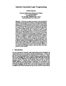
4. Results To determine the performance of BiGGER relative to the FFT approach, we compared the search time with that reported with ZDock for the immunoglobulin complex between IgG1 Idiotypic Fab and Igg2A anti-idiotypic Fab [12]. For this complex the authors reported a run time of 19 CPU hours on an SGI Origin 2000 with 32 R10000 processors, for a search through 6,389 orientations. The performance of each R10000 processor in the SGI Origin workstation is roughly a third (SSBENCH floating point benchmark) to a fourth (SPECfp95 and SPECfp2000) of the performance of a Pentium 4 2.8GHz CPU for floating point operations, so this allows us to make an approximate comparison between the two algorithms. To compare the algorithms we ran BiGGER on the same protein complex as reported in [12] (PDB structure codes 1AIF and 1IAI) at different resolutions to generate different grid sizes (the resolution is the size of the grid cell). The reason for using the same structure is that running time for BiGGER depends slightly on the shape and relative sizes of the docking partners, so in our comparisons with ZDock changes occur in only one variable, the size of the grid. Chart A on Figure 7 shows the plot of the average for 10 orientations for BiGGER for each grid size (black dots) compared to the estimated time for ZDock on a similar platform, represented by the staircase plot. The FFT algorithm requires the grid to be decomposed into shorter sequences, so N must be factorable into powers of small prime numbers for FFT to be usable; ideally, N should be a power of 2. This results in a staircase-like performance plot, using the values of N for which FFT is most efficient. To simplify the plot, we represented the computation time for ZDock on the relevant N values where N is a power of two (64, 128, 256, 512). In protein docking it is unlikely that values outside this range are necessary. Chart B (Figure 7) shows the experimental results using only the propagation of the surface overlap constraint (section 3.1) or both surface and core overlap constraints (sections 3.1 and 3.2). The experimental results are compared with the naïve O(N6) complexity of comparing all the grids in all configurations, and the O(N4) complexity estimated for BiGGER as the grid size tends to infinity. The real-space (geometrical) search in BiGGER seems to be at least as efficient in computation time as the FFT approach, and significantly more efficient in those cases where the size of the structures is just enough to force the grid size in the FFT to a larger increment of N. This conclusion is valid for the practical range of grid sizes used in protein docking, though with a time complexity of O(N4), which is slightly worse than the O(N3Log(N)) of FFT, BiGGER eventually becomes slower than FFT as grid size increases. However, the space complexity of BiGGER is O(N2), except for fractal shapes, whereas the memory requirements for the FFT approach are O(N3), and the necessity of using floating point matrices makes it very demanding in this regard. With a 256 grid size and double precision, FFT docking requires 130Mb per grid. Since 3 grids are necessary, one for each protein and one for the correlation matrix, this amounts to approximately 500Mb, or 8Gb for N=512. The grid representation in BiGGER requires only a few megabytes, and the total memory usage of the program is approximately 10Mb of RAM at running time (15Mb for the largest example in the chart with N=330, 5Mb for the smallest with N=42). Space complexity may be as

relevant as time complexity because the geometric search is trivial to parallelize, since each orientation in the rotation space can be explored independently. 1000

N

N

FFT (Zdock)

10

BiGGER

1

0.1

B

N

N

6

4

100 Time (Seconds).

100 Time (Seconds).

1000

4

6

A

10 Surface Surface+Core

1

0.1

0.01

0.01 0

100

200 Grid Size

300

400

0

100

200

300

400

Grid Size

Fig. 7. Plots of search time as a function of the grid size. Chart A compares BiGGER (dots) to the estimated time for a FFT implementation (ZDock) on the same hardware. Chart B compares BiGGER with only the surface overlap constraint (Section 3.1) and both the surface and core overlap constraints (section 3.1 and 3.2). Both charts also show the theoretical values for O(N6) and O(N4) complexities assuming a constant scaling factor such that both correspond to the estimated factor for the ZDock implementation of the FFT method at N=40.

The other advantage of our approach is the possibility of reducing the search space according to information about the interaction of the two proteins. Previous publications showed the advantages of using such information to score the models generated [4, 10, 11], without using this information to narrow the search, so here we address only the performance gains in restricting the search space with the algorithm described in section 3.4, using as example the CAPRI [1] targets 2 and 4 through 7, corresponding to our submitted predictions for CAPRI rounds 1 and 2 [4]. For the largest protein on each pair of proteins to dock we selected five alphaCarbon atoms: three from the three interface residues that we had used to test the models obtained with an unconstrained search in [4], plus two from two decoy residues picked at random away from the interface region. The constraint imposed on the search was that at least 3 of the alpha-Carbon atoms of these five residues on the largest protein must be within 10Å of at least one atom of the smallest protein, which restricts the search the region of the three correct residues and away from the region with the two decoys. Even this modest information has a significant effect on the quality of the prediction of the protein complex, as shown in [4]. Here we focus exclusively on the performance issues of using the constraints to prune the search space, as a proper discussion of the evaluation of protein complex models would be outside the scope of this paper. Table 1 shows the residues selected as correct interface residues and decoys for each protein, and the time for the constrained search as a fraction of the time for the unconstrained search. The total time for the constrained search (through 6,389 orientations) ranged from three and a half hours for ID 2 to 30 minutes for ID 6 (approximate results on a P4 at 2.8 GHz running Windows XP ™) The time gains depend on how much the search space is pruned by the constraint, so it will depend on the shape and size of the structures as well as the number and

placement of the distance constraints and the stringency of the cardinality constraint over the distances to enforce. Still, these results suggest a significant reduction in computation time (two to five times) even when constraining only a few points on only one of the partners. With more stringent constraints, such as requiring that one specific point on one structure be close to one of a few points in the other, the constrained search time can be less than 5% of the unconstrained search time (for example, 23 minutes instead of 12 hours in the case of complex ID 2).

ID Complex 2 VP6-FAB 4 Amilase-Amy10 5 Amilase-Amy07 6 Amilase-Amy09 7 Exotoxin A1-TC AR

Correct Residues P171,A244,M300 S243,S245,G249 S270,G271,G285 N53,S145,V349 N20,N54,Y84

Decoys D62,G43 N364,D375 R30,N220 S471,T219 N178,G108

Constr. 210 40 90 30 80

Unconst. 720 160 180 150 180

Table 1. Shows the residues selected as correct interface residues and decoys for each CAPRI target, and the time of the constrained and unconstrained searches in minutes.

5. Conclusion By taking advantage of Constraint Programming techniques, BiGGER is faster than the FFT correlation method for matching three-dimensional shapes for N up to approximately 500. With larger grids, the O(N4) time complexity of BiGGER eliminates the advantage of simpler and faster operations, making it slower than the FFT algorithm with its O(N3Log(N)) time complexity. However, at large grid sizes the O(N3) space complexity of FFT is a severe disadvantage compared to the O(N2) space complexity of BiGGER. Although we cannot state categorically that, on performance alone, our approach is superior to the FFT method, this shows that our algorithm is at a similar performance level as the currently most popular approach for modelling protein-protein complexes. The main advantage of BiGGER is in being suited for the efficient implementation of a wide range of constraints on distances between parts of the structures to fit, which is often important in protein docking, and potentially important in other problems of finding optimal surface matches between complex shapes subject to geometrical constraints. For the problem of protein docking, in which we are most interested, the algorithm has been applied successfully to model the interaction between a Pseudoazurin and a Nitrite Reductase [16] and is currently being applied to modelling two other protein interactions (Fibrinogen-MMP2 and FNR-Ferredoxin) with promising results. Acknowledgements: We thank Nuno Palma and José Moura for their role in the development of BiGGER and Chemera, and we thank the financial support of the Fundação para a Ciencia e Tecnologia (BD 19628/99; BPD 12328/03).

References 1.

2.

3. 4. 5.

6.

7.

8.

9.

10.

11.

12. 13.

14. 15. 16.

Palma PN, Krippahl L, Wampler JE, Moura, JJG. 2000. BiGGER: A new (soft) docking algorithm for predicting protein interactions. Proteins: Structure, Function, and Genetics 39:372-84. Katchalski-Katzir E, Shariv I, Eisenstein M, Friesem AA, Aflalo C, Vakser IA. 1992 Molecular surface recognition: determination of geometric fit between proteins and their ligands by correlation techniques. Proc Natl Acad Sci U S A. 1992 Mar 15;89(6):2195-9. Janin J. 2002. Welcome to CAPRI: A Critical Assessment of PRedicted Interactions. Proteins: Structure, Function, and Genetics Volume 47, Issue 3, 2002. Pages: 257 Krippahl L, Moura JJ, Palma PN. 2003. Modeling protein complexes with BiGGER. Proteins: Structure, Function, and Genetics. V. 52(1):19-23. Dominguez C, Boelens R, Bonvin AM. HADDOCK: a protein-protein docking approach based on biochemical or biophysical information. J Am Chem Soc. 2003 Feb 19;125(7):1731-7. Moont G., Gabb H.A., Sternberg M. J. E., Use of Pair Potentials Across Protein Interfaces in Screening Predicted Docked Complexes Proteins: Structure, Function, and Genetics, V35-3, 364-373, 1999 Pettigrew GW, Goodhew CF, Cooper A, Nutley M, Jumel K, Harding SE. 2003, The electron transfer complexes of cytochrome c peroxidase from Paracoccus denitrificans. Biochemistry. 2003 Feb 25;42(7):2046-55. Pettigrew GW, Prazeres S, Costa C, Palma N, Krippahl L, Moura I, Moura JJ. 1999. The structure of an electron transfer complex containing a cytochrome c and a peroxidase. J Biol Chem. 1999 Apr 16;274(16):11383-9. Pettigrew GW, Pauleta SR, Goodhew CF, Cooper A, Nutley M, Jumel K, Harding SE, Costa C, Krippahl L, Moura I, Moura J. 2003. Electron Transfer Complexes of Cytochrome c Peroxidase from Paracoccus denitrificans Containing More than One Cytochrome. Biochemistry 2003, 42, 11968-81 Morelli X, Dolla A., Czjzek M, Palma PN, Blasco, F, Krippahl L, Moura JJ, Guerlesquin F. 2000. Heteronuclear NMR and soft docking: an experimental approach for a structural model of the cytochrome c553-ferredoxin complex. Biochemistry 39:2530-2537. Morelli X, Palma PN, Guerlesquin F, Rigby AC. 2001. A novel approach for assessing macromolecular complexes combining soft-docking calculations with NMR data. Protein Sci. 10:2131-2137. Chen R. & Weng Z. 2002 Docking Unbound Proteins Using Shape Complementarity, Desolvation, and Electrostatics, Proteins 47:281-294 Ten Eyck, L. F., Mandell, J., Roberts, V. A., and Pique, M. E. Surveying Molecular Interactions With DOT. Proceedings of the 1995 ACM/IEEE Supercomputing Conference, San Diego A. Vakser, C. Aflalo, 1994, Hydrophobic docking: A proposed enhancement to molecular recognition techniques, Proteins, 20, 320-329. Krippahl L, Barahona P. PSICO: Solving Protein Structures with Constraint Programming and Optimisation, Constraints 2002, 7, 317-331 Impagliazzo, A., Transient protein interactions: the case of pseudoazurin and nitrite reductase. 2005. Doctoral Thesis, Leiden University