2: Basic stages of the statistical classification process. 2.1.1 Pre-Processing. The data obtained from fMRI neuro-imaging are especially rich and complex [7] and ...
International Conference in Distributed Computing & Internet Technology (ICDCIT-2013) Proceedings published in International Journal of Computer Applications® (IJCA) (0975 – 8887)
Applying Machine Learning Techniques for Cognitive State Classification Shantipriya Parida
Satchidananda Dehuri
Carrier Software & Core Network Huawei Technologies India Pvt Ltd Bangalore, India
Department of Systems Engineering Ajou University, San 5, Woncheon-dong Yeongtong-gu, suwon 443-749, South Korea
ABSTRACT One of the key challenges in cognitive neuroscience is determining the mapping between neural activities and mental representations. The functional magnetic resonance imaging (fMRI) provides measure of brain activity in response to cognitive tasks and proved as one of the most effective tool in brain imaging and studying the brain activities. The complexities involved in fMRI classification are: high dimensionality of fMRI data, smaller size of the dataset, interindividual differences, and dependence on data acquisition techniques. The state-of-the-art machine learning techniques popularly used by neuroimaging community for variety of fMRI data analysis has created exciting possibilities to understand deeply the functioning of inner structure of the human brain. In this paper, we present an overview of different stages involved in cognitive state classification and focuses on different machine learning approaches, their worthiness, and potentiality in identifying brain states into pre-specified classes. The machine learning techniques ranges from conventional to recent hybrid techniques which have shown promising result in fMRI classification are discussed here. Further, this paper suggests direction for further research in this area by synergizing with other related fields.
General Terms Functional Magnetic Resonance Imaging, Principal Component Analysis, Independent Component Analysis, Bayesian classifier, Support Vector Machine, Linear Discrimination Classifier
Keywords Multi-band Connectivity Graphs, Supervised Clustering
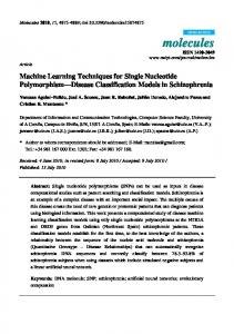
1. INTRODUCTION The fMRI is an extension to the conventional magnetic resonance imaging (MRI) used for detail analysis of neural activity and provide extensive understanding of the relationship between brain activation and subjective human experience [1]. The fMRI technique is based on the measurement of the neural activity through the change in blood oxygen level [2]. It provides a sequence of 3D brain images representing blood oxygenation level dependent (BOLD) brain activations. The obtained brain images are used by machine learning techniques to design decoders to classifying brain states [3] [4] [5]. Figure 1 shows the 3dimensional image of 64x64x34 voxels [6].
Fig. 1: 3-dimensional image of voxels [6]
The basic cognitive task includes the following.
Feature Extraction Pattern Discovery Statistical Inference
The above cognitive tasks discussed with respect to machine learning in the following sections.
2. MACHINE LEARNING APPROACHES FOR COGNITIVE STATE CLASSIFICATION In this paper, the following machine learning approaches are focused based on their performance and applicability in cognitive state classification.
Statistical classification approach, Neural network approach, Kernel based approach, Multiband connectivity graph approach, Supervised clustering approach.
2.1 Statistical Classification Approach The statistical classification approach uses the statistical pattern recognition method for classification, recognition, and identification. The steps include in statistical classification process is shown in Fig. 2.
Fig. 2: Basic stages of the statistical classification process
2.1.1 Pre-Processing The data obtained from fMRI neuro-imaging are especially rich and complex [7] and fMRI generates vast amount of data which are becoming a challenge for machine learning and data mining researchers [8]. Prior to analysis, fMRI data typically undergoes a series of preprocessing steps aimed at removing artifacts and validating model assumptions. Preprocessing or
40
International Conference in Distributed Computing & Internet Technology (ICDCIT-2013) Proceedings published in International Journal of Computer Applications® (IJCA) (0975 – 8887) voxel selection is a common step in many pattern-based classification models of functional neuro-imaging data [9]. The steps involved in fMRI preprocessing are slice timing correction, realignment, co-registration of structural and functional images, normalization, and smoothing [10] (see Figure 3).
decomposition of fMRI time series formulated as the estimation of both matrices of the right side of the following equation:
Xc = A. C,
(1)
subject to the constraint that the processes Ci are spatially independent.
2.1.3 Feature Selection
Fig 3: The fMRI data processing pipeline illustrate the steps involved in a standard fMRI experiment [10]
2.1.2 Feature Extraction The feature extraction creates new features as a function of existing features as shown in Fig. 4. It is one of the form dimensionality reductions. Although in fMRI many algorithms exist for feature selection, the challenges in feature extraction lies in finding common features for the entire subject in the data set and method best fit to the experimental design and classification.
The feature selection is vital in cognitive classification as it is computationally infeasible to use all the available features [13]. The feature selection algorithms search the best feature subset within the set of features aims to reduce the classification error based on various criteria i.e. for a set of 𝐷 features, the algorithm selects a subset of size 𝑑 < 𝐷, which has the greatest potential to discriminate between classes. The feature selection is effective in reducing dimensionality, removing irrelevant data, increasing learning accuracy and improving result comprehensibility. The feature selection techniques broadly divided into wrappers, filters and Embedded. Wrapper: The wrapper approach based on the classifier accuracy where the possible feature subsets input to the model and the subset for which the model perform best is selected. Filter: The filter approach does not depend on the performance of the model for which it’s much faster compared to wrapper approach. Embedded: In this method the variable selection happens in the process of training and usually this method specific to given learning machines.
Fig. 4: Feature extraction The principal component analysis (PCA) and independent component analysis (ICA) are widely used for feature extraction and dimensionality reduction. PCA is the bestknown unsupervised linear feature extraction algorithm.
2.1.2.1 Principal Component Analysis (PCA) The data involve in fMRI scan seen as continuous functions of time sampled at the interscan interval resulting observational noise and used to estimate an image where smooth functions replace the voxels. The functional data analysis techniques are used to apply PCA directly on these functions. The common technique used in PCA is identifying Eigen values (amount for variation) and Eigen vectors (direction of variance) of the covariance matrix of the data [11].
2.1.2.2 Independent Component Analysis (ICA) It is one of the popular techniques for fMRI signals capable of revealing connected brain systems of functional significance [12]. In contrast to conventional statistical methods applied in fMRI analysis, ICA is data-driven and multivariate. The decomposition is determined solely by the intrinsic spatio– temporal structure of the data set, i.e. no a priori assumption about the time profile of the effects of interest is required. Let Xc be the T × Mc (T = number of scans, Mc = number of cortical time-courses) matrix of the observed cortical time courses, C the N × Mc matrix whose rows Ci (i = 1, …, N) contain the spatial processes (N T = number of processes) and A the T N mixing matrix whose columns Aj ( j = 1, …, N ) contain the time courses of the N processes. The ICA-
The following general methods used for selecting informative features with respect to fMRI data analysis [14]. Activity: Selects voxels which are active in at least one condition relative to a control task baseline, the voxel score measured by a t-test on the difference in mean activity level between condition and baseline. Accuracy: Scores a voxel by how accurately a Gaussian Bayesian classifier can predict the condition of each example in the training set, based only on the voxel. Searchlight Accuracy: Same as the Accuracy, but apart from using the data from a single voxel, it uses data from the voxel and its immediately adjacent neighbors in three dimensions. Analysis of Variance (ANOVA): Looks for voxels where there are reliable differences in mean value across conditions (e.g. A is different from B C D, or AB from CD, etc) as measured by an ANOVA. Stability: Picks voxels that react to the various conditions consistently across cross-validation groups in the training set (e.g. if the mean value in A is less than B and greater than C, is this repeated in all groups).
2.1.4 Learning Classifiers One of the popular techniques used in recent development is machine learning classifiers for classifying cognitive states analyzing the fMRI data. The trained classifier represents a function of the form [15]:
41
International Conference in Distributed Computing & Internet Technology (ICDCIT-2013) Proceedings published in International Journal of Computer Applications® (IJCA) (0975 – 8887)
Φ ∶ 𝑓𝑀𝑅𝐼 𝑡, 𝑡 + 𝑛 → 𝑌,
(2)
where 𝐟𝐌𝐑𝐈 𝐭, 𝐭 + 𝐧 is the observed fMRI data during the interval from time t to 𝐭 + 𝐧, and 𝐘 is a finite set of cognitive states to be discriminated. 𝚽 𝐟𝐌𝐑𝐈 𝐭, 𝐭 + 𝐧 the classifier prediction regarding which cognitive state gave rise to the observed fMRI data 𝐟𝐌𝐑𝐈 𝐭, 𝐭 + 𝐧 . The classifiers proved their worthiness for cognitive classifications are:
Gaussian Naïve Bayes(GNB) Classifier Support Vector Machine(SVM) k-Nearest Neighbor(kNN) Linear Discrimination Classifier (LDC)
The GNB classifier uses the training data to estimate the probability distribution over fMRI observations, conditioned on the subject’s cognitive state [16]. It then classifies the new example x = x1 … xn by estimating the probability P ci x of cognitive state ci given fMRI observation x. It estimates this P ci x using Bayes rule, along with the assumption that the features xj are conditionally independent given the class:
P ci Пj P xj ci k
P ck Пj P x j ck
Given row vectors a and x with m features, and their means μa, μb and standard deviation σa , σb the distances/similarities most commonly used are
euclidean2 a, x = a − x a − x ′ ax′ = a x′ a x a − μa x − μx) corelation a, x = m − 1 σa σx
(4)
cosine a, x =
2.1.4.1 Gaussian Naïve Bayes (GNB) Classifier
P ci x =
finding the training set example which is closest to it by some measure (e.g. Euclidean distance) and assigning its label to the test example. With concern to accuracy and stability the kNN is better for MRI data compared to common statistical classifier and found as a relevant technique for segmenting MRI brain abnormalities [18].
(3)
where P denotes distributions estimated by the GNB from the training data. Each distribution of the from P xj ci is modeled as a univariate Gaussian, using maximum likelihood estimates of the mean and variance derived from the training data. Given a new example to be classified, the GNB outputs posterior probabilities for each cognitive state, calculated using the above formula.
2.1.4.2 Support Vector Machine (SVM) The SVM is one of the most popular and state-of-the-art maximum classification algorithm used in fMRI studies. For two classes, the SVM algorithm find a linear decision boundary (separating hyperplane) using the decision function as shown in Fig. 4. The fMRI classification uses the experimental design as the class label such as stimulus A, and stimulus B assigned unique class. The experiment consists of a series of brain images which is being collected for class label changes.
Fig. 5: The geometric interpolation of linear SVMs (H denotes for the hyperplane, S denotes for the support vector) [17].
2.1.4.3 k-Nearest Neighbour (k-NN) It is the simplest classifier in its kind where no parameters are learnt. The classification of test example is performed by
=
(5) ′
(6)
a x′ m−1
where x is a normalized version of the data vector x (making it norm 1 for cosine similarity or z-scored, i.e. mean 0 and standard deviation 1, for correlation similarity.
2.1.4.4 Linear Discrimination Classifier (LDC) The LDC belongs to the generative group of classifiers where the classes assumed to have normal distribution and equal covariance matrices. The optimal classifier reduces to calculating linear discriminant function for each class which is stimulus in case of fMRI experiment. For a given object x (brain state at a given time) is obtained by the tag of the largest discriminant function [19].
2.2 Classifier Evaluation The simplest form of evaluation is in terms of classification accuracy.
2.2.1 The holdout method The simplest method is to take your original dataset and partition it into two, randomly selecting instances for a training set (usually 2/3 of the original dataset) and a test set (1/3 of the dataset). The classifier builds using the training set and then evaluates it on the ‘held-out’ test set. The holdout, method can be made more reliable by repeating it several times, with randomly selected training and test sets each time.
2.2.2 k-Fold Cross Validation In k-fold cross-validation, the original dataset is first partitioned into k subsets of equal size, 𝐏𝟏 , … , 𝐏𝐤 . Each subset is used in turn as the test set, with the remaining subsets being the training set. In other words, first 𝐏𝟐 , … , 𝐏𝐤 form the training set and 𝐏𝟏 is the test set; second 𝐏𝟏 , 𝐏𝟑 . . . , 𝐏𝐤 form the training set and 𝐏𝟐 is the test set; and so on; finally, on the kth fold, 𝐏𝟏 , … , 𝐏𝐤−𝟏 . form the training set and 𝐏𝐤 is the test set. The accuracies from each of the‘folds’ are averaged to given an overall accuracy. This avoids the problem of overlapping test sets and makes very effective use of the available data.
2.2.3 Leave-one-out crosses Validation Leave-one-out cross-validation is a special case of k-fold cross-validation in which k = n, where n is the size of the original dataset. Hence, the test sets are all of size 1. In other words, first instances 𝐱 𝟐 , … , 𝐱 𝐧 form the training set and 𝐱 𝟏 is the only test instance; second 𝐱 𝟏 , 𝐱 𝟑 , … 𝐱 𝐧 form the
42
International Conference in Distributed Computing & Internet Technology (ICDCIT-2013) Proceedings published in International Journal of Computer Applications® (IJCA) (0975 – 8887) training set and 𝐱 𝟐 is the only test instance; and so on; finally, on the nth fold, 𝐱 𝟏 , … , 𝐱 𝐧−𝟏 form the training set and xn is the only test instance. This makes the best use of the available data and avoids the problems of random selections.
2.3 Neural Network Classification Approach In Artificial Neural Network (ANN), a sort of machine learning implementation has been applied to a broad range of fMRI problem. Here we describe the Multi Layer Perception (MLP)-based classification that is essential for describing its application to fMRI [20]. The Fig. 6 shows a representative model of a MLP neural network.
A set of synaptic weights connections: a signal xj in input synapse j, connected to the neuron k, is multiplied by the weight synapse wkj ; Input signals, weighted by the correspondingly synaptic weights, are summed with other input signals on a linear combination fashion; An activation function that limits the amplitude of output signals. The activation function φ(.) defines the output neurons in terms of active signal level in its input and provides a nonlinear characteristic to the MLP.
Φ v =
1 1+e α v
(7)
Fig. 7: The pre-processing of the fMRI data. The black boxes are the key processing steps used in fMRI analysis, while the blue boxes are noise filter and hypothesis-driven feature extraction technique [21]
2.5 Multiband Connectivity Graph approach One more recent approach for brain state classification proposed by Richiardi et al. [22] is multi-band classification of connectivity graphs. The main task of this approach as follows. Estimate connectivity at different temporal scales using the wavelet transform as a preprocessing step(see Figure 8). Build classifier trained on functional connectivity graphs of a group of subjects to distinguish between brain states of an unseen subject. It identifies the connections that are most discriminative between brain states.
Fig. 6: MLP Neural Network Model [20]
2.4 Kernel based approach Recently, kernel based techniques have shown promising results when applied to fMRI analysis for predicting continuous brain states. Typically, a training data set would consist of a series of several hundred volumetric fMRI scans (images), where each scan is a volume of around 64x64x34 voxels. Kernels are essentially square, symmetric and positive definite matrices that encode measures of similarity between each pair of scans.
Fig. 8: Flow chart of the preprocessing procedure. DWT stands for discrete wavelet transform [22]
The useful properties of kernel method is
The kernel trick reduces the computational complexity for high dimensional data as the parameter evaluation domain is reduced from the explicit feature space into the kernel space. With an appropriate kernel function one can map the input feature space into higher dimensions. This allows non-linear approaches in the original feature space to be achieved by linear approaches in the higher dimensional space
Fig. 9: Views of discriminative graphs. Connections with darker colors and thicker lines correspond to more discriminative ability [22]
The Fig. 7 shows an instance of kernel method for brain activity prediction.
43
International Conference in Distributed Computing & Internet Technology (ICDCIT-2013) Proceedings published in International Journal of Computer Applications® (IJCA) (0975 – 8887) The classification obtained deriving the training samples and grows the decision tree using leave-one-subject-out cross validation procedure. The combining decisions of the classifiers in each sub band obtain higher accuracy than the best single band classifier.
Fig. 12: Illustration of the supervised clustering algorithm on a simple simulated data set [23]
3. FUTURE PERSPECTIVES Fig. 10: Flowchart of the classification and ensembling procedure [22]
2.6 Supervised Clustering approach To reduce the dimensionality, Michel et al. [23] proposed a new supervised clustering approach for brain state inference from fMRI image. In the proposed supervised clustering approach, they first constructed a hierarchical subdivision of the search domain using Ward hierarchical clustering algorithm. The output parcel sets constructed from the functional data is isomorphic to a tree and by construction; there is a one-to-one mapping between cuts of this tree and parcellations of the domain. Given a parcellation, the signal can be represented by parcel-based averages, thus providing a low dimensional representation of the data. The steps for the supervised clustering approach as follows. 1.
Bottom-Up step (Ward clustering): The tree T is constructed from the leaves(the voxels in the gray box) to the unique root (full brain volume), following spatial connectivity constraints
2.
Top-Down step(Pruning of the tree):The Ward’s tree is cut recursively into smaller sub-trees, each one corresponding to a parcellation, in order to maximize a prediction accuracy
3.
Model selection: Given the set of nested parcellations, obtained by the pruning step, select the optimal sub-tree
Although the discussed classification techniques proved their worthiness in different application such as lie detection [24], brain activity prediction [25], brain computer interface [26], mental disorder discovery [27]. Still there exist many opportunities for analyzing fMRI data and improving classification accuracy. The new kernel based approach [21] which was tested for single subject learning and shown great improvement in brain activity prediction can further extended to multiple subject for various cognitive activities. The multiband connectivity approach [22] which shown to be applicable for inter-subject brain decoding with low error rate can further extended for more sophisticated segmentation method. The supervised clustering approach [23] which obtained better prediction accuracy can extended to use in any dataset where multi-scale structure is considered. Apart from the above mentioned scope of research of the discussed techniques, some of the potential areas of research in cognitive state classification include [28],
Finding new feature selection method for such high dimensional and periodically changing data.
Improved classifier for multi subject classification with high accuracy.
Explore the applicability of the classifier approach to diagnostic classification problems, such as early detection of mental disease (e.g., Alzheimer, Parkinson). Finding structure underlying high-dimensional neural representations. Relating one person’s neural patterns to another’s.
One of the promising areas in fMRI classification which can further extended is applying hybrid techniques as the hybrid classifier tries to use the desirable properties of each individual classifier and emphasizes to improve the overall accuracy in the combined approach [29] [30].
4. CONCLUSION Fig. 11: Flowchart for supervised clustering approach [23] The illustration of the supervised clustering algorithm as follows(see Figure 12) . The cut of the tree (top, red line) focuses on the regions of the interest (top, green dots), which allows the prediction function to correctly weight the informative features.
This paper explained various machine learning approaches like statistical, neural, kernel based, multiband connectivity graph, and supervised clustering techniques. Additionally, we studied their feasibility in brain state inference using fMRI observations. The most useful machine learning classifiers for cognitive state classification, their efficiencies, and challenges are focused as a part of this study. The scope of research for
44
International Conference in Distributed Computing & Internet Technology (ICDCIT-2013) Proceedings published in International Journal of Computer Applications® (IJCA) (0975 – 8887) the discussed techniques and potential areas in cognitive classification are highlighted in this paper.
5. REFERENCES [1] Savoy, R. L. 1996. Functional magnetic resonance imaging (fMRI). Encyclopedia of Neuroscience, 2nd ed. Boston, MA: Birkhauser. [2] Onut, I. V., Ghorbani, A. A. 2004. Classifying Cognitive States from fMRI Data using Neural Networks. in Proc. IEEE Joint Conf. Neural Networks, vol. 4, 2871-2875. [3] Zanzotto, F. M., Croce, D. 2010. Comparing EEG/ERPlike and fMRI-like Techniques for Reading Machine Thoughts. in Proc. 2010 Int. Conf. Brain Informatics, Berlin, Germany: Springer-Verlag, 133-144. [4] Naselaris, T., Kay, K. N., Nishimoto, S., Gallant, J. L. 2011. Encoding and decoding in fMRI. NeuroImage, vol. 56, no. 2, 400-410. [5] Mitchell, T. M., Hutchinson, R., Niculescu, R. S., Pereira, F., Wang, X. 2004. Learning to Decode Cognitive States from Brain Images. Machine Learning, vol. 57, no. 1-2, 145-175. [6] Schmaler, C. 2008. Infering cognition from fMRI brain images A machine learning approach. Sequence Learning Seminar SS08. [7] Horwitz, B., Tagamets, M., McIntosh, A. R. 1999. Neural modeling, functional brain imaging, and cognition. Trends in Cognitive Sciences, vol. 3, no. 3, 91-98. [8] Nielsen, F. A., Christensen, M. S., Madsen, K. H. Lund, T. E., Hansen, L. K. 2006. fMRI Neuroinformatics. IEEE Engineering in Medicine and Biology Magazine, vol. 25, no. 2, 112-119. [9] O’Toole, A. J., Abdi, F. J. H., Penard, N., Dunlop, J. P., Parent, M. A. 2007. Theoretical, statistical, and practical perspectives on pattern-based classification approaches to the analysis of functional neuroimaging data. Cognitive NeuroScience, vol. 19, 1735-1752. [10] Lindquist, M. A. 2008. The Statistical Analysis of fMRI Data Statistical Science, vol. 23, no. 4, 439-464. [11] Viviani, R., Gron, G., Spitzer, M. 2005. Functional principal component analysis of fMRI data. Human Brain Mapping, vol. 24, 109-129. [12] Anderson, A., Bramen, J., Douglas, P. K., Lenartowicz, A., Cho, A., Culbertson, C., Brody, A. L., Yuille, A. L., Cohen, M. S. 2011. Large Sample Group Independent Component Analysis of Functional Magnetic Resonance Imaging Using Anatomical Atlas-Based Reduction and Bootstrapped Clustering. Int. J. Imaging Syst Technol. vol. 21, no. 2, pp. 223–231. [13] Kohavi, R., John, G. H. 1997. Wrappers for Feature Subset Selection. Artificial Intelligence, vol. 97, no. 1-2, 273-324. [14] Pereira, F., Mitchell, T., Botvinick, M. 2009. Machine learning classifiers and fMRI: a tutorial overview. NeuroImage, vol. 45, no.1 Suppl., S199-S209. [15] Mitchell, T. M., Hutchinson, R., Just, M. A. Niculescu R. S., Wang, X. 2003. Classifying Instantaneous Cognitive States from fMRI data. in American Medical Informatics Association Symposium, 465-469.
[16] Mitchell, T. M., Hutchinson, R., Niculescu, R. S., Pereira, F., Wang X. 2004. Learning to Decode Cognitive States from Brain Images. Machine Learning, vol. 57, no. 1-2, 145-175. [17] Zhang, Y., Wu, L. 2012. An MR brain images classifier via principal component analysis and kernel support vector machine. Progress In Electromagnetics Research, vol. 130, pp. 369-388. [18] Khalid, N. E. A., Ibrahim, S., Haniff, P. N. M. M. 2011. MRI brain abnormalities segmentation using K-nearest neighbors (k-NN). Int. J. Computer Science Engineering, vol. 3, no. 2. [19] Kuncheva, L. I., Rodriguez, J. J. 2010. Classifier Ensembles for fMRI data Analysis: An Experiment. Magnetic Resonance Imaging, vol. 28, no. 4, 583-593. [20] Espirito-Santo, R. D., Sato, J. R., Martin, M. G. M. 2007. Discriminating brain activated area and predicting the stimuli performed using artificial neural network. Exacta, Sao Paulo, vol. 5, no. 2, 311-320. [21] Ni, Y., Chu, C., Sunders, C. J., Ashburner, J., 2008. Kernel Methods for fMRI Pattern Prediction. in Proc. IEEE Int. Joint Conf. Neural Networks, 692-697. [22] Richiardi, J., Eryilmaz, H., Schwartz, S., Vuilleumier, P., Ville, D. V. D. 2011. Decoding brain states from fMRI connectivity graphs. NeuroImage, vol. 56, no. 2, 616626. [23] Michel, V., Gramfort, A., Varoquaux, G., Eger, E., Keribin, C., Thirion, B. 2011. A supervised clustering approach for f-MRI based inference of brain states. CoRR abs/1104.5304. [24] Davatzikos, C., Ruparel, K., Fan, Y., Shen, D. G., Acharyya, M., Loughed, J. W., Gur, R. C., D. D. Langleben, D. D. 2005. Classifying spatial patterns of brain activity with machine learning methods: Application to lie detection. NeuroImage, vol. 28, no. 3, 663-668. [25] Boehm, O., Hardoon, D. R., 2011. Classifying cognitive states of brain activity via one-class neural networks with feature selection by genetic algorithms. Int. Journal of Machine Learning & Cybernetics, vol. 2, no. 3, 125-134. [26] deCharms, R. C. 2008. Application of real-time fMRI. Nature Reviews Neuroscience, vol. 9, No. 9, 720-729. [27] Liu, X., Liu, B., Chen, J., Chen, Z. 2011. Functional magnetic resonance imaging of regional homogeneity changes in parkinsonian resting tremor. Neural Regeneration Research, vol. 6, no. 11, 811-815. [28] Raizada, R. D. S., Kriegeskorte, N. 2010. Patterninformation fMRI: new questions which it opens up, and challenges which face it. Int. J. Imaging Systems Technology, vol. 20, no. 1, 31-41. [29] Wang, Z. 2009. A hybrid SVM-GLM approach for fMRI data analysis. NeuroImage, vol. 46, no. 3, 608-615. [30] Yang, H., Liu, J., Sui, J., Pearlson, G., Calhoun, V. D. 2010. A hybrid machine learning method for fusing fMRI and genetic data: combining both improves classification for schizophrenia. Frontiers in Human Neuroscience, vol. 4.
45