Applying Non-Negative Matrix Factorization on ...

Applying Non-Negative Matrix Factorization on Time-Frequency Reassignment Spectra for Missing Data Mask Estimation Maarten Van Segbroeck∗, Hugo Van hamme Katholieke Universiteit Leuven, Department of Electrical Engineering – ESAT Kasteelpark Arenberg 10, B-3001 Leuven, Belgium {maarten.vansegbroeck,hugo.vanhamme}@esat.kuleuven.be

Abstract The application of Missing Data Theory (MDT) has shown to improve the robustness of automatic speech recognition (ASR) systems. A crucial part in a MDT-based recognizer is the computation of the reliability masks from noisy data. To estimate accurate masks in environments with unknown, non-stationary noise statistics, we need to rely on a strong model for the speech. In this paper, an unsupervised technique using non-negative matrix factorization (NMF) discovers phone-sized time-frequency patches into which speech can be decomposed. The input matrix for the NMF is constructed using a high resolution and reassigned time-frequency representation. This representation facilitates an accurate detection of the patches that are active in unseen noisy speech. After further denoising of the patch activations, speech and noise can be reconstructed from which missing feature masks are estimated. Recognition experiments on the Aurora2 database demonstrate the effectiveness of this technique. Index Terms: noise robust speech recognition, missing data techniques, mask estimation, speech separation, non-negative matrix factorization

1. Introduction Additive noise results in a decrease in performance of ASRsystems due to the mismatch between the speech models obtained in clean conditions and the statistics of speech in the noisy test conditions. Missing Data Techniques have shown their effectiveness in reducing this mismatch. In the MDT approach, a missing data detector decides for each frame which features of the noisy speech are unreliable (missing) or reliable. The latter are treated as clean speech data in the acoustic models of the recognizer’s back-end. The missing features on the other hand are either marginalized or their value is estimated from the reliable data using the state distribution of the ASR as a prior (data imputation), see [1]. For reasons of accuracy, the ASRsystem operates in a domain that is a linear transformation of log-spectra. Therefore, the data imputation technique needs to be extended to cover such linear transformations. An alternative MDT formulation was presented in [2] through the introduction of the ProSpect features and will be briefly restated in section 2. One of the main advantages of missing data techniques over other noise reduction methods is that less assumptions need to be made about the noise type. Therefore, more constraints should be placed on the speech model. In this paper, the speech model consists of a collection of recurring acoustic patterns that are discovered and learned without supervision from clean ∗

This work was supported by “Institute for the Promotion of Innovation through Science and Technology in Flanders (IWTVlaanderen)”.

speech data. The learning algorithm involved makes use of nonnegative matrix factorization (NMF) introduced by [3]. Thanks to the non-negativity constraints, NMF decomposes a matrix in additive (not subtractive) components, resulting in a partsbased representation of the data. NMF can therefore be seen as a learning algorithm that, when applied to an appropriate feature space, finds the parts or objects that the training data are built of. This approach was also used in a variety of other researches, see e.g. [4, 5, 6]. As will be explained in section 3, the patterns are discovered from a combination of two complementary feature representations that either reveal timing or frequency structure and which are derived from a reassigned timefrequency representation (RTFR) [7]. This allows the NMF to find patterns that reveal localized time-frequency structures in high resolution speech spectra. The advantage of learning patterns from a RTFR is that it facilitates the detection of these patterns in unseen noisy test utterances, e.g. the reassignment method improves the localization of the spectral energy in time and frequency, which already separates the speech to some extent from additive noise sources. The acoustic patterns will be referred to as time-frequency patches of speech and are highly interpretable on an acoustic and a phonetic basis. The patches can also model the dynamic spectro-temporal characteristics of speech, such as formant transitions. The proposed missing data detector (MDD) will exploit this speech model by first retrieving the patches that are present in the high resolution representation of the noisy speech. Therefore, a noise model is also involved to explain the presence of the noise in the speech. This approach was also followed in [8] to improve the accuracy of the patch activations. The noise model can be trained offline or online during recognition. It suffices that this noise model roughly captures the spectral shape of the noise and it does not have to be representative for different levels of signal-to-noise ratio (SNR) in noisy speech. After a denoising procedure of the patch activations where only those patches are selected with highest activation energy, we can reconstruct the speech and the noise. Finally, these high resolution spectra are transformed into a low resolution representation in order to construct the missing feature masks for the MDTbased recognizer. A description of the proposed MDD will be outlined in section 4. The experiments on the Aurora2 connected digit recognition task demonstrates the success of our system and are presented in section 5. Conclusions are given in section 6.

2. Missing Data Techniques The speech recognizer is assumed to have a mainstream HMMbased architecture with Gaussian mixture models (GMM). In the front-end, a low resolution Mel-spectral representation is computed by a filter bank with D channels through windowing,

4

3

3

kHertz

kHertz

4 2 1 100

1 300

kHertz

2 1 100

200

300

400

300

400

2 1 100

200

300

400

time [ms]

4

3

200

time [ms]

3

400

time [ms]

4

100 4

2

200

1

400

kHertz

kHertz

300

3

100

kHertz

200

time [ms]

4

3.1. Time-frequency reassignment

2

3 2 1 100

time [ms]

200

300

400

time [ms]

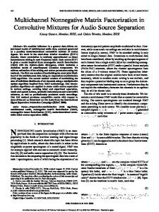
Figure 1: STFT representation (top), RTFR (middle) and enhanced RTFR (bottom) for the word “two” with focus on timing (left) and frequency (right) structure. In the bottom left panel, vertical lines correspond to plosive and vocal fold bursts, while the enhanced RTFR at the bottom right reveals the horizontal structure in the word, e.g. pitch and formant contours. framing, FFT and filter bank integration. At a certain frame, let s, n and y denote the vector of log-Mel spectral features for clean speech, noise and noisy signal respectively. In a missing data approach, the components of y are divided into a reliable, y r , and an unreliable part, y u . The reliable components of s are approximated by y r . In the maximum likelihood per-Gaussian-based imputation [2], the missing part of s is estimated by minimizing the (negative) log-likelihood for each Gaussian mixture component over s: 1 (s − µ)′ P (s − µ) (1) 2 subject to the equality and inequality constraints: sr = y r and su ≤ y u

(2)

where µ is the Gaussian mean and P is an inverse covariance or precision matrix, both estimated on clean training data. In most MDT systems, GMMs with diagonal covariance in the log-spectral domain are used, resulting in a diagonal structure for P and a tractable maximum likelihood estimation for s. Higher accuracies are obtained with GMMs with a diagonal covariance in the cepstral domain, in which case P becomes nondiagonal. Imputation then becomes computationally more complex since the estimation of the unreliable part now requires the solution of a Non-Negative Least Square problem. In this paper, the ProSpect features defined in [2] will be used. Just like cepstra, they are computed by a linear transform of the logarithm of the filter bank energies. While these features can be applied in any speech recognition system, they show especially a clear benefit in MDT-based recognition since they reduce the computational requirements over cepstral MDT while the accuracy is maintained.

3. Discovery of time-frequency patches The production of human speech can be regarded as a process of combining a small number of spectral patterns into many more different sequences. In this section, our goal is to find a set of patterns by analyzing continuous speech recordings. Therefore, we transform the speech data into a time-frequency reassignment spectrogram [7] on which we perform a non-negative matrix factorization (NMF). By imposing non-negativity constraints, NMF generates parts that are additive, unlike factorization techniques such as PCA or SVD. The finally obtained speech patterns are acoustic time-frequency patches of correlated energy.

Time-frequency reassignment [7, 9] allows perfect localization of (well-separated) impulses, cosines and chirps, which constitute a reasonable model for speech. The corresponding reassigned time-frequency representation (RTFR) has an increased sharpness of localization of the signal components without sacrificing the frequency resolution. The RTFR is obtained by moving the spectral density value away from the point in the time-frequency plane where it was computed. It can be applied to different time-frequency representations each characterized by a different analysis kernel. In a RTFR, energy is reallocated from the geometric center of the spectral analysis kernel function to the center of gravity of the energy distribution. In this paper, the reassignment principle is applied to the short time Fourier transform (STFT). Let H(t, ω), D(t, ω) and T (t, ω) denote the STFT of the signal obtained with the window of choice h(t), the derivative of h(t) and the time weighted th(t) respectively and let ℜ(X) and ℑ(X) be the real and imaginary part of X, then the energy at (t, ω) is reassigned to the center of gravity [7]: – » –« „ » ` ´ D(t, ω) T (t, ω) ,ω −ℑ (3) tˆ, ω ˆ = t+ℜ H(t, ω) H(t, ω) where the time and frequency offsets are computed from the ratios of the three STFTs. To improve the visibility of acoustic events with short duration, we further enhance the localization of the energy along the time axis. Therefore, we first search for zero-crossing points in the time offsets of (3) and only those of them that are connected in the vertical direction (i.e. along the frequency axis) are retained. Finally, the corresponding energy of the RTFR is assigned to the retained points. When applied to speech with a sufficiently short analysis window, the enhanced RTFR clearly shows the vertical (i.e. well-localized in time) lines that are related to the burst of plosives and affricatives and energy releases by the vocal folds. By repeating the same procedure using the frequency offsets of (3), the tracks of time-varying spectral features such as pitch and formants can be clearly localized in frequency. We have found that formant structure is more apparent if we use shorter windows in the RTFR. The different steps of the enhanced reassignment procedure are shown figure 1 for the word “two”. Firstly, a time-frequency representation is computed using a N -point STFT (N = 128). Subsequently, a RTFR is produced by reallocating the spectral energy to the gravity centers according to (3). The above mentioned enhancement steps are then applied to the RTFR to reveal either the timing or the frequency structure. Experiments have shown that an optimal choice for the window length is respectively 11 ms and 7 ms for male speakers and 6 ms and 4 ms for female speakers. The analysis window is shifted by 1 ms. Experiments not included in this paper due to space constraints, have revealed that the enhanced RTFR is more robust than the STFT and produces better results for the approaches that will be described next. 3.2. Constructing the input matrix In this section, we explain how the input matrix is created to which we will apply NMF for finding acoustic time-frequency patterns in speech signals. These patterns are discovered on clean training data. After pre-emphasizing the speech signals, we compute the enhanced RTFRs by the approach described in section 3.1. Both representations will be used to exploit the spectral information that is more apparent in either the vertical or the horizontal direction.

Freq. Bins

128 96

3.4. Time-frequency patches of speech

64 32

Freq. Bins

1

2

3

4

5

6

7

8

9

10

17

18

19

20

Basic Units Index

128 96 64 32 11

12

13

14

15

16

Patch Index

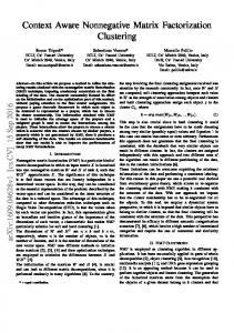
Figure 2: A collection of the discovered time-frequency patches with a duration of 60 ms. Some patches correspond to formant patterns and formant transitions (top row); others model interphone or silence-phone transitions, bursts and wideband spectra (bottom row). Let us now define the spectral vector at a certain time t as v t and ht , corresponding to the feature representation that reveals respectively the timing (vertical) and frequency (horizontal) structure. These representations will contain complementary information and therefore both are combined in the input matrix to discover the speech patches. Let us now define the real and non-negative column vector of dimension N as ct = max(v t , ht ) (4) where the max-operator works element-wise. At each time step t, we take k consecutive columns of ct representing the spectrotemporal structure of a short-time speech segment (i.e. of length k ms). These k columns are reshaped into a single column vector Ct of dimension kN , from which we construct a data matrix C of size kN × T by concatenating T columns from the clean training set. 3.3. Matrix factorization for unsupervised learning By applying non-negative matrix factorization to the matrix C, it is approximated by: C ≈ BA (5) subject to the constraint that all matrices are non-negative and where the common dimension of B and A is much smaller than T and kN . Hence, equation (5) contains only additive linear combinations such that the factorization leads to a parts-based representation. These parts are found in the columns of B and their activation across time are given by the corresponding rows of A. To retrieve a sparse representation of the data and to assure that each basic vector models a different time-frequency pattern, additional sparsity constraints must be enforced on A. Therefore, we use sparse NMF [10] where the factorization is approximated by minimizing the objective function: X G(C||BA, λ) = D(C||BA) + λ Aij (6) i,j

where the left term of (6) is the generalized version of the Kullback-Leibler divergence [3], while the right term in equation (6) enforces sparsity on A by minimizing the L1 -norm of its columns. The trade-off between reconstruction accuracy and sparseness is controlled by the parameter λ. An algorithm for finding B and A given C based on multiplicative updates and with the additional sparseness constraint, can be found in [11]. To address scaling, the constraint that each column of B sums to unity is imposed. Experiments have shown that with the settings used in this paper, a good choice for λ is 1000. Alternatively, convolutive NMF could be used to obtain a parts-based representation of the data [11]. Although this variant is appealing from a theoretical point of view, experiments, not reported in this paper, have shown that the activations of these patches are less robust to additional noise sources.

The columns of matrix B correspond to spectral patches which describe the recurrent time-varying spectra of speech. A set of 1000 time-frequency patches were discovered from the training set as described above with a patch length of 60 ms. A selection of these patches are shown in figure 2. Most patches describe formant movements over the duration of about a phone. A smaller set of time-frequency patches are modeling the beginning or ending of phones and phone-pair transitions. Others resemble wideband sounds and short-time energy bursts. Experiments have shown that a patch duration of 60 ms is optimal to obtain the recognition results of section 5.

4. NMF-based mask estimation In the MDD, the high resolution RTFR of the noisy speech is described in terms of the discovered time-frequency patches. Patch activations are then computed and express to what extent each patch is present across time. To improve the accuracy of the activation matrix, some denoising steps are also performed during this process. From the final selected patches, speech and noise are reconstructed to estimate the spectral mask. 4.1. Denoising of patch activations during testing To discover the patches that are present in test utterances of the Aurora2 database, the same procedure is used as in training except that we compute A in equation (5) by holding B fixed to the one obtained from training. However, to prevent that some of the speech patches are activated to explain the noise in the unseen noisy speech, some modifications are required during this process. Firstly, an extra noise model is included to explain the presence of additive noise sources. This noise model can be trained offline using the same method as described in section 3 or can be trained online. If we refer to the speech model with Bs , to the noise model with Bn and use the subscript y to denote the noisy speech, than we can write: – » ˆ ˜ As . (7) Cy ≈ B s B n An A second necessary step to further denoise the speech activation matrix As is similar to a winner-takes-all strategy and is done during the iterative computation of eq. (7). Once convergence is reached, we select only those patches of Bs and Bn with highest activation. Therefore, we zero out, per column of As and An , all the rows that do not correspond to these patches. Due to the property of the multiplicative update rules, these patches stay unactivated in further iterations. To this end, the total energy of speech and noise will be redistributed over the patches that are most probable to describe speech and noise. In our experiments, 15 iterations are sufficient to reach convergence using a full activation matrix after which 5 iterations are performed using only the patches with highest activation energy. 4.2. Constructing the mask Once equation (7) is solved using the additional denoising steps as mentioned in the previous section, we can reconstruct the data matrix of speech Cs ≈ Bs As and noise Cn ≈ Bn An . After reshaping these matrices and a weighted summation to obtain N -dimensional high resolution spectra, a smoothing in time and frequency is performed to convert these spectra into a low resolution time-frequency representation. Time smoothing is performed by reframing with a sliding triangular window of 30 frames and a frameshift of 10 frames, after which a

mask type

SNR (dB) 15 binary 10 5 15 fuzzy 10 5

Oracle masks Subw. Babble Car Exhib. 98.96 98.73 99.11 98.89 97.70 98.19 97.82 96.73 93.34 95.50 92.07 90.28 98.77 98.58 98.78 98.52 97.67 97.94 98.42 97.13 94.66 96.01 94.09 91.92

Avg. 98.92 97.61 92.80 98.66 97.79 94.17

Table 1: Recognition accuracy (%) on Aurora2 test set A using ProSpect MDT with binary and fuzzy oracle masks. mask type

SNR (dB) 15 binary 10 5 15 fuzzy 10 5

Harmonicity masks Subw. Babble Car Exhib. 97.61 97.04 98.12 97.87 94.87 93.29 95.02 93.86 83.14 81.92 81.90 79.51 97.61 97.40 98.33 98.09 95.12 94.50 95.47 94.14 85.97 85.37 83.48 81.73

mask type

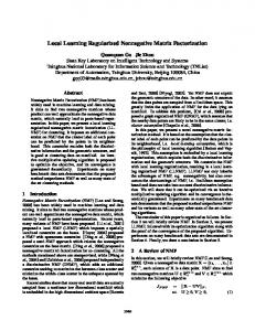
SNR (dB) 15 binary 10 5 15 fuzzy 10 5

NMF-based masks Subw. Babble Car Exhib. 97.88 97.22 98.39 97.66 95.39 95.10 95.02 94.11 88.95 87.22 86.88 86.15 97.97 97.61 98.54 98.24 95.70 95.59 96.00 94.82 89.13 88.97 88.25 87.47

Avg. 97.79 94.90 87.30 98.10 95.53 88.46

Table 3: Recognition accuracy (%) for NMF-based masks.

6. Conclusions Avg. 97.66 94.26 81.62 97.86 94.81 84.14

Table 2: Recognition accuracy (%) for harmonicity masks. Mel-scaled filterbank is applied to smooth in the frequency domain. After logarithmic compression, the reconstructed spectra for speech and noise approximate the log-Mel feature vectors as ˆ and n ˆ respectively. used in section (2) and will be denoted by s Finally, the missing data masks are constructed by substituting these estimates into the binary or fuzzy mask decision criterion [12], i.e. respectively 1 ` ´ ˆ