Jul 29, 2013 - Decimation algorithm is excellent. The algorithmic rate-distortion curve approaches the optimal curve of the ensemble as the width.
1
Approaching the Rate-Distortion Limit with Spatial Coupling, Belief propagation and Decimation Vahid Aref, Nicolas Macris and Marc Vuffray
arXiv:1307.5210v2 [cs.IT] 29 Jul 2013
School of Computer and Communication Science Ecole Polytechnique F´ed´erale de Lausanne LTHC - IC - EPFL - Station 14 CH - 1015 Lausanne, Switzerland
Abstract—We investigate an encoding scheme for lossy compression of a binary symmetric source based on simple spatially coupled Low-Density Generator-Matrix codes. The degree of the check nodes is regular and the one of code-bits is Poisson distributed with an average depending on the compression rate. The performance of a low complexity Belief Propagation Guided Decimation algorithm is excellent. The algorithmic rate-distortion curve approaches the optimal curve of the ensemble as the width of the coupling window grows. Moreover, as the check degree grows both curves approach the ultimate Shannon rate-distortion limit. The Belief Propagation Guided Decimation encoder is based on the posterior measure of a binary symmetric testchannel. This measure can be interpreted as a random Gibbs measure at a “temperature” directly related to the “noise level of the test-channel”. We investigate the links between the algorithmic performance of the Belief Propagation Guided Decimation encoder and the phase diagram of this Gibbs measure. The phase diagram is investigated thanks to the cavity method of spin glass theory which predicts a number of phase transition thresholds. In particular the dynamical and condensation “phase transition temperatures” (equivalently test-channel noise thresholds) are computed. We observe that: (i) the dynamical temperature of the spatially coupled construction saturates towards the condensation temperature; (ii) for large degrees the condensation temperature approaches the temperature (i.e. noise level) related to the information theoretic Shannon test-channel noise parameter of rate-distortion theory. This provides heuristic insight into the excellent performance of the Belief Propagation Guided Decimation algorithm. The paper contains an introduction to the cavity method. Index Terms—Lossy source coding, rate-distortion bound, Low-Density Generator Matrix codes, Belief Propagation, decimation, spatial coupling, threshold saturation, spin glass, cavity method, density evolution, dynamical and condensation phase transitions.
I. I NTRODUCTION
L
OSSY source coding is one of the oldest and most fundamental problems in communications. The objective is to compress a given sequence so that it can be reconstructed up to some specified distortion. It was established long ago [1] that Shannon’s rate distortion bound for binary sources (under Hamming distance) can be achieved using linear codes. However, it is of fundamental importance to find low complexity encoding schemes that achieve the rate distortion limit. An early attempt used trellis codes [2], for memoryless sources and bounded distortion measures. It is possible to approach
the Shannon limit as the trellis constraint length increases, but the complexity of this scheme, although linear in the block length N , becomes exponential in the trellis constraint length. In [3] an entirely different scheme is proposed (also with linear complexity and diverging constants) based on the concatenation of a small code and optimal encoding of it. More recently, important progress was achieved thanks to polar codes [4] which were shown to achieve the rate-distortion bound with a successive cancellation encoder of complexity O(N ln N ) [5]. Further work on the efficient construction of such codes followed [6]. Another interesting recent direction, that is also the one investigated in this paper, uses Low-Density Generator-Matrix (LDGM) codes, for which Belief Propagation (BP) and/or Survey Propagation (SP) equipped with a decimation process yield low complexity1 encoding schemes. Using a plain message passing algorithm without decimation is not effective in lossy compression. Indeed the estimated marginals are either nonconverging or non-biased because there exists an exponentially large number of compressed words that lead to roughly the same distortion. In this respect the lossy compression schemes based on random graphs are an incarnation of random constraint satisfaction problems and, from this perspective it is not too surprising that their analysis share common features. The general idea of BP or SP guided-decimation algorithms is to: i) Compute approximate marginals by message passing; ii) Fix bits with the largest bias, and if there is no biased bit take a random decision; iii) Decimate the graph and repeat this process on the smaller graph instance. For naive choices (say regular, or check-regular) of degree distributions the Shannon rate-distortion limit is not approached by such algorithms. However it has been observed that it is approached for degree distributions that have been optimized for channel LDPC coding [7], [8], [9]. These observations are empirical: it is not clear how to analyze the decimation process, and there is no real principle for the choice of the degree distribution. In this contribution we investigate a simple spatially coupled LDGM construction. The degree distributions that we consider are regular on the check side and Poisson on the codebit side. The average of the Poisson distribution is adjusted to achieve the desired compression rate. We explore a low 1 O(N 2 )
or O(N ) depending on the exact implementation.
complexity Belief Propagation Guided Decimation (BPGD) encoding algorithm, that takes advantage of spatial coupling, and approaches the Shannon rate-distortion limit for large check degrees and any compression rate. No optimization on the degree distributions is needed. The algorithm is based on the posterior measure of a test binary symmetric channel (BSC). We interpret this posterior as a random Gibbs measure with an inverse temperature parameter equal to the halflog-likelihood parameter of the test-BSC. This interpretation allows us to use the cavity method of spin glass theory in order to investigate the phase diagram of the random Gibbs measure. Although the cavity method is not rigorous, it makes definite predictions about the phase diagram of the measure. In particular it predicts the presence of phase transitions that allow to gain insight into the reasons for the excellent performance of the BPGD encoder on the spatially coupled lossy compression scheme. Spatially coupled codes were first introduced in the context of channel coding in the form of convolutional LDPC codes [10] and it is now well established that the performance of such ensembles under BP decoding is consistently better than the performance of the underlying ensembles [11], [12], [13]. This is also true for coupled LDGM ensembles in the context of rateless codes [14]. The key observation is that the BP threshold of a coupled ensemble saturates towards the maximum a posteriori MAP threshold of the underlying ensemble as the width of the coupling window grows. A proof of this threshold saturation phenomenon has been accomplished in [15], [16]. An important consequence is that spatially coupled regular LDPC codes with large degrees universally achieve capacity. Recently, more intuitive proofs based on replica symmetric energy functionals have been given in [17], [18]. Spatial coupling has also been investigated beyond coding theory in other models such as the Curie-Weiss chain, random constraint satisfaction problems [19], [20], [21], and compressed sensing [22], [23], [24]. Let us now describe in more details the main contents of this paper. Summaries have appeared in [25], [26]. In [25] we had investigated regular spatially coupled graph constructions with constant degrees for both check and code-bits. The performance of the BPGD algorithm are similar to the case of Poisson degree for code-bit nodes, on which we will concentrate here. In section II we set up the framework for lossy source coding with spatially coupled LDGM ensembles for a binary symmetric Bernoulli source and Hamming distortion. We investigate ensembles with regular check degrees and Poisson code-bit node degrees. Important parameters of the spatial constructions are the number of positions L, the number of nodes n at each position, and the window width w over which we couple the nodes. The infinite block length limit investigated in this paper corresponds to limL→+∞ limn→+∞ in the specified order. Optimal encoding consists in finding the compressed word that minimizes the Hamming distortion between a given source realization and the reconstructed word. Since we will use methods from statistical mechanics, we will translate the problem in this language. Optimal encoding can be viewed as the search for the minimum energy
configurations of a random spin Hamiltonian. Although the optimal encoder is computationally impractical, it is important to determine the optimal distortion of the ensemble in order to set a limit on what cannot be achieved algorithmically for the ensemble. In this respect, an important rigorous result that is reviewed in section II is that, in the infinite block length limit limL→+∞ limn→+∞ , for any fixed w the optimal distortion for a spatially coupled ensemble is equal to the optimal distortion for the underlying uncoupled ensemble (and is therefore independent of w). This result follows from an equivalent one proved in [21] for the random XORSAT problem for any values of the constraint density. There are various results in the literature about the optimal encoder for the uncoupled ensemble. So we can essentially transfer them directly to our spatially coupled setting. In [7] it is proven by second moment methods that, LDGM based codes with Poisson degrees for code-bit nodes and regular degree for check nodes, achieve the ultimate Shannon rate-distortion limit under optimal encoding when the check degrees grow large. A similar conclusion was reached (by non-rigorous means) from the cavity [27] and replica [28] methods from statistical physics. These studies also showed that the gap to the ratedistortion bound vanishes exponentially in the large check degree limit. As explained in section II optimal encoding can be viewed as the study of the zero temperature limit of the Gibbs measure associated with a Hamiltonian. This Gibbs measure forms the basis of the BP based algorithms that we use. This Gibbs measure is nothing else than the posterior measure of the dual test-channel problem, and that the inverse temperature is the half-log-likelihood parameter of a test-BSC2 . The free energies of the spatially coupled and underlying ensembles are the same [21] in the infinite block length limit (fixed w) and therefore their static phase transition temperature (the condensation temperature) is also the same (see below). The Gibbs measure (or posterior measure of the dual test-channel problem) is the basis for setting up the BPGD algorithms. This is explained in detail in Section III. The crucial point is the use of the spatial dimension of the graphical construction. The main idea is that when the biases are small a random bit from the boundary of the chain is fixed to a random value, and as long as there exist bits with large biases they are eliminated from the chain by fixing them and decimating the graph. We consider two forms of BPGD. The first one, which as it turns out performs slightly better, is based on hard decisions. The second one uses a randomized rounding rule for fixing the bits. Sections IV reviews the simulation results and discusses the performance for the two versions of the BPGD encoders. For both algorithms we observe that the rate-distortion curve of the coupled ensemble approaches the Shannon limit when n >> L >> w >> 1 and the node degrees get large. We cannot assess if the Shannon limit is achieved based on our numerical results. However we observe that in order to avoid finite size effects the degrees have to become large only 2 More precisely, if p is the flip parameter of the BSC test-channel then the ). inverse temperature is β = 12 ln( 1−p p
after the other parameters grow large in the specified order. In practice though n = 2000, L = 64, w = 3 and check degrees equal to l = 3 yield good results for a compression rate 1/2. The performance of the BPGD algorithms depend on the inverse temperature parameter in the Gibbs measure, and one can optimize with respect to this parameter. Interestingly, for the coupled ensemble, we observe that for large degrees (when Shannon’s rate-distortion limit is approached) the optimal parameter corresponds to the information theoretic value of the flip probability given by the Shannon distortion. This is non-trivial: indeed it is not true for the uncoupled ensemble. The behavior of BPGD algorithms is to some extent controlled by the phase transitions in the phase diagram of the Gibbs measure. In section V we review the predictions of the cavity method, and in particular the predictions about the dynamical and condensation phase transition temperatures. At the condensation temperature the free energy displays a singularity and is thus a thermodynamic or static phase transition threshold. The dynamical temperature on the other hand is not a singularity of the free energy, but Markov Chain Monte Carlo algorithms have an equilibration time which diverges at (and below) this temperature. Similarly, BPGD with randomized rounding correctly samples the Gibbs measure down to temperatures slightly higher than the dynamical threshold. We observe a threshold saturation phenomenon for the spatially coupled construction. First as said above, since the condensation threshold is a singularity of the free energy it is the same for the uncoupled and coupled ensembles for any w. Second, as the window width w grows the dynamical threshold saturates towards the condensation one. In practice we observe this saturation for values of w as low as w = 3, 4, 5. Thus for spatially coupled codes the BPGD algorithm is able to correctly sample the Gibbs measure down to a temperature approximately equal to the condensation threshold. This explains why the algorithm performs well, indeed it is able to operate at much lower temperatures than in the uncoupled case. A large degree analysis of the cavity equations shows that the condensation temperature tends to the information theoretic value corresponding to the flip parameter of the BSC test-channel given by Shannon’s distortion. These facts, put together, provide insight as to the excellent performance of the BPGD algorithm for the spatially coupled ensemble. Section VI presents the cavity equations for the coupled ensemble on which the results of the previous paragraph are based. These equations are solved by population dynamics in Section VII. The cavity equations take the form of six fixed point integral equations. However we observe by population dynamics that two of them are satisfied by a trivial fixed point. This is justified by a theoretical analysis in section VIII. When this trivial fixed point is used the remaining four equations reduce to two fixed point integral equations which have the form of usual density evolution equations for a BSC channel. This simplification is slightly surprising because although the original Gibbs measure does not possess channel symmetry3 this symmetry emerges as a solution of the cavity equations. Within this framework the saturation of the 3 In
the context of spin glass theory this is the Nishimori gauge symmetry.
dynamical temperature towards the condensation one appears to be very similar than threshold saturation in the context of channel coding with LDPC codes. For an introduction to the cavity theory we refer the reader to the book [29]. This theory is not easy to grasp both conceptually and technically. This paper contains a high level introduction of the main concepts in Section V and a summary of the main technical ideas in Appendix A. We hope that this will be helpful for unfamiliar readers. The necessary derivations and adaptations to the present setting of a spatially coupled Gibbs measure are summarized in Appendices B and C. The main sections II-V and the conclusion can be read without explicitly going into the cavity formalism. II. C OUPLED LDGM E NSEMBLES FOR LOSSY COMPRESSION
A. Lossy Compression of Symmetric Bernoulli Sources Let X = {X1 , X2 , . . . , XN } represent a source of length N , where Xa , a = 1, . . . , N are i.i.d Bernoulli(1/2) random variables. We compress a source word x by mapping it to one of 2N R index words u ∈ {0, 1}N R , where R ∈ [0, 1] is the compression rate. This is the encoding operation. The decoding operation maps the stored sequence u to a reconstructed sequence x b(u) ∈ {0, 1}N . b), we measure the distortion by the For a given pair (x, x relative Hamming distance dN (x, x b) =
N 1 X |xa − x ba | . N a=1
(1)
The quality of reconstruction is measured by the average distortion DN (R) = EX [dN (x, x b)] (2) where EX is the expectation with respect to the symmetric Bernoulli source. For the symmetric Bernoulli source considered here, it is well-known that for any encoding-decoding scheme, the average distortion is lower bounded by Shannon’s rate-distortion curve [30] Dsh (R) = h−1 (3) 2 (1 − R) where h2 (x) = −x log2 x − (1 − x) log2 (1 − x) is the binary entropy function. The rate-distortion curve is convex decreasing with Dsh (0) = 1/2 and Dsh (1) = 0. B. Spatially Coupled Low-Density Generator Matrix Constructions Our lossy source coding scheme is based on a spatially coupled LDGM code ensemble. We first describe the underlying ensemble. 1) Underlying Poisson LDGM(l, R) Ensemble: These are bipartite graphs with a set C of n check nodes of constant degree l, a set V of m code-bit nodes of variable degree, and a set E of edges connecting C and V . The ensemble of graphs is generated as follows: each edge emanating from a check node is connected uniformly at random to one of the code-bit nodes. The degree of code-bit nodes is a random variable with
x1 x2 x3 x4 x5
x b1 x b2 x b3 x b4 x b5
x6 x7
x b6 x b7
x8
x b8
for i ∈ V , ∂i = {a ∈ C| (i, a) ∈ E}. For spatially coupled graphs the sets of nodes at a specified position z are Cz and Vz .
u1 u2 u3
C. Decoding Rule and Optimal Encoding
u4
We “attach” a code bit ui to each code-bit node i ∈ V . To each check node a ∈ C we “attach” two type of bits: the reconstructed bit x ba and the source bit xa . By definition the source sequence has length N . So we have n = N for the underlying ensembles, and nL = N for the coupled ensembles. A compressed word u has length m for the underlying ensemble, and m(L + w − 1) for the coupled ensemble. Thus the compression design rate is R = m/n for the underlying ensemble, and it is Rcou = m(L + w − 1)/nL = R(1 + w−1 L ) for the coupled ensemble. The compression design rate of the coupled ensembles is slightly higher, due to the codebit nodes at the boundary, but in the asymptotic regime n, m >> L >> w the difference with the design rate R of the underlying ensemble vanishes. 1) Decoding Rule: The reconstruction mapping is given by the linear operation (modulo 2 sum)
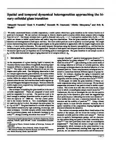
Fig. 1. A bipartite graph from the underlying LDGM(2, 0.5) ensemble. Here n = 8, m = 4 and l = 2. Labels represent code-bits ui , reconstructed bits x ˆi and source bits xi .
boundary set
boundary set
w=2 Fig. 2. The ”protograph” representation of the spatially coupled LDGM(2, 0.5, L = 8, w = 2) ensemble. The code-bit nodes in boundary sets have smaller degree than the code-bit nodes in the other sets.
Binomial distribution Bi(ln, 1/m). In the asymptotic regime of large n, m with m/n = R the code-bit node degrees are i.i.d Poisson distributed with an average degree l/R. 2) Spatially Coupled LDGM(l, R, L, w, n) Ensemble: We first lay out a set of positions indexed by integers z ∈ Z on a one dimensional line. This line represents a “spatial dimension”. We fix a “window size” which is an integer w ≥ 1. Consider L sets of check nodes each having n nodes, and locate the sets in positions 1 to L. Similarly, locate L + w − 1 sets of m code-bit nodes each, in positions 1 to L + w − 1. All checks have constant degree l, and each of the l edges emanating from a check at position z ∈ {1, . . . , L} is connected uniformly at random to code-bit nodes within the range {z, . . . , z + w − 1}. It is easy to see that for z ∈ {w, . . . , L − w + 1}, in the asymptotic limit n → +∞, the code-bit nodes have Poisson degrees with average l/R. For the remaining positions close to the boundary the average degree is reduced. More precisely for positions on the left side z ∈ {1, . . . , w − 1} the degree is asymptotically i.i.d Poisson with average l/R × z/w. For positions on the right side z ∈ {L + 1, . . . , L + w − 1} the degree is asymptotically Poisson with average l/R × (L + w − z)/w. Figures 1 and 2 give a schematic view of an underlying and a spatially coupled graph. 3) Notation: Generic graphs from the ensembles will be denoted by Γ or Γ(C, V, E). We will use letters a, b, c for check nodes and letters i, j, k for code-bit nodes of a given graph (from underlying or coupled ensembles). We will often make use of the notation ∂a for the set of all code-bit nodes connected to a ∈ C, i.e. ∂a = {i ∈ V | (i, a) ∈ E}. Similarly,
x ba (u) = ⊕i∈∂a ui .
(4)
In this paper we do not investigate non-linear decoding rules, although the whole analysis developed here can be adapted to such rules. Source coding with such “non-linear check nodes” have been investigated for underlying LDGM(l, R) ensembles [31]. 2) Optimal Encoding: Given a source word x, the optimal encoder seeks to minimize the Hamming distortion (1), and so searches among all u ∈ {0, 1}N R to find a configuration u∗ such that b(u)) . u∗ = argminu dN (x, x
(5)
The resulting minimal distortion is dN,min (x) = min dN (x, x b(u)) . u
(6)
3) Optimal Distortion of the Ensemble: A performance measure is given by the optimal distortion of the ensemble (not to be confused with Shannon’s optimal distortion) DN,opt = ELDGM,X [dN,min (x)]
(7)
where ELDGM,X is an expectation over the graphical ensemble at hand and the symmetric Bernoulli source X. Finding the minimizers in (5) by exhaustive search takes exponential time in N ; and there is no known efficient algorithmic procedure to solve the minimization problem. Nevertheless, the cavity method proposes a formula for the asymptotic value of (7) as N → +∞. It is conjectured that this formula is exact. We come back to this point at the end of paragraph II-D.
D. Statistical Mechanics Formulation NR
We equip the configuration space {0, 1} with the condiNR tional probability distribution (over u ∈ {0, 1} ) 1 e−2βN dN (x,bx(u)) Zβ (x) 1 Y −2β|xa −Li∈∂a ui | = e Zβ (x)
3
4
5
6
Dopt
0.1179
0.1126
0.1110
0.1104
TABLE I
O PTIMAL DISTORTION FOR LDGM(l, R = 0.5) ENSEMBLES COMPUTED IN [31]; S HANNON ’ S BOUND FOR R = 0.5 IS Dsh ≈ 0.1100.
µβ (u | x) =
(8)
a∈C
where β > 0 is a real number and X e−2βN dN (x,bx(u)) Zβ (x) =
l
(9)
There exists also another useful relationship that we will use between average distortion and free energy. Consider the ”internal energy” defined as b(u))i] uN (β) = 2ELDGM,X [hdN (x, x
u
(15)
a normalizing factor. The expectation with respect to u is denoted by the bracket h−i. More precisely the average of a function A(u) is X 1 hA(u)i = e−2βN dN (x,bx(u)) . (10) Z N
It is straightforward to check that the internal energy can be computed from the free energy (use (9), (14), (15)) ∂ uN (β) = (βfN (β)) (16) ∂β and that in the zero temperature limit it reduces to the average minimum energy or optimal distortion (use (6), (7), (15))
An important function that whose average we consider below is the distortion of a pair (x, x b(u)), A(u) = dN (x, x b(u)). Note that the minimizer u∗ in (5) maximizes this conditional distribution, (11) u∗ = argmaxu µβ (u | x) .
2DN,opt = lim uN (β).
u∈{−1,+1}
The source coding problem can thus be interpreted as an estimation problem where x is an observation and u has to be estimated. In this paper we prefer the statistical mechanics interpretation, because we use related methods and concepts. Equation (8) defines the Gibbs distribution associated to a ”spin glass” Hamiltonian 2N dN (x, x b(u)). This Hamiltonian is a costfunction for assignments of ”dynamical” variables, the spins (or bits) ui ∈ {0, 1}. The Hamiltonian is random: for each realization of the source sequence x and the graph instance we have a different realization of the cost-function. The source and graph instance are qualified as ”quenched” or ”frozen” random variables, to distinguish them from dynamical variables, because in physical systems - as well as in algorithms - they fluctuate on vastly different time scales. The parameter β is the “inverse temperature” in appropriate units, and the normalizing factor (9) is the partition function. Finding u∗ amounts to find the ”minimum energy configuration”. The minimum energy per node is equal to 2dN,min , and it is easy to check the identity (use 6 and 9) 2dN,min (x) = − lim
β→∞
1 ln Zβ (x) . βN
(12)
As this identity already shows, a fundamental role is played by the average free energy fN (β) = −
1 ELDGM,X [ln Zβ (x)]. βN
(13)
For example the average free energy allows to compute the optimal distortion of the ensemble 2DN,opt = lim fN (β). β→+∞
(14)
β→+∞
(17)
What is the relation between the quantities fN (β), uN (β), and DN,opt for the underlying and coupled ensembles? The following theorem states that they are equal in the infinite block length limit. This limit is defined as lim
N →+∞
= lim
n→+∞
with m/n fixed for the underlying ensemble; and as lim
N →+∞
= lim
lim
L→+∞ n→+∞
with m/n fixed for the coupled ensemble. We stress that for the coupled ensemble the order of limits is important. Theorem 1. Consider the two ensembles LDGM(l, R, n) and LDGM(l, R, L, w, n) for an even l and R. Then the respective limits limN →+∞ fN (β), limN →+∞ uN (β) and limN →+∞ DN,opt exist and have identical values for the two ensembles. This theorem is proved in [21] for the max-XORSAT problem. The proof in [21] does not depend on the constraint density, so that it applies verbatim to the present setting. We conjecture that this theorem is valid for a wider class of graph ensembles. In particular we expect that it is valid for odd l and also for the regular LDGM ensembles (see [32] for similar results concerning LDPC codes). It is conjectured that the one-step-replica-symmetrybreaking-formulas (1RSB), obtained from the cavity method [33], for the N → +∞ limit of the free, internal and ground state energies are exact. Remarkably, it has been proven [34], using an extension of the Guerra-Toninelli interpolation bounds [35], that these formulas are upper bounds. The 1RSB formulas allow to numerically compute [31], using population dynamics, Dopt ≡ limN →+∞ DN,opt . As an illustration, Table I reproduces Dopt for increasing check degrees. Note that Dopt approaches Dsh as the degrees increase. One observes that with increasing degrees the optimal distortion of the ensemble attains Shannon’s rate-distortion limit.
III. B ELIEF P ROPAGATION G UIDED D ECIMATION Since the optimal encoder (5) is intractable, we investigate suboptimal low complexity encoders. In this contribution we focus on two encoding algorithms based on the belief propagation (BP) equations supplemented with a decimation process. 1) Belief Propagation Equations: Instead of estimating the block u (as in (5)) we would like to estimate bits ui with the help of the marginals X µi (ui | x) = (18) µβ (u | x) where the sum is over u1 , . . . uN with ui omitted. However computing the exact marginals involves a sum with an exponential number of terms and is also intractable. For sparse random graphs, when the size of the graph is large, any finite neighborhood of a node i is a tree with high probability. As is well known, computing the marginals on a tree-graph can be done exactly and leads to the BP equations. It may therefore seem reasonable to compute the BP marginal distribution in place of (18), ui 1 eβ(−1) ηi 2 cosh βηi
(19)
where the biases ηi are computed from solutions of the BP equations. The later are a set of fixed point equations involving 2 |E| real valued messages ηi→a and ηba→i associated to the edges (i, a) ∈ E of the graph. We have ( � Q ηba→i = (−1)xa β −1 tanh−1 tanh β j∈∂a\i tanh βηj→a P ηi→a = b∈∂i\a ηbb→i (20) and ηi =
X
ηba→i .
(21)
a∈∂i
For any solution of the BP equations one may consider the estimator u bBP = argmaxui µBP i i (ui | x) ( 1 (1 + sign tanh βηi ), if ηi 6= 0 = 2 Bernoulli( 21 ), if ηi = 0.
(i,a)∈E
for some t < T , then tdec = t. ii) If (23) does not occur for all t ≤ T then tdec = T . (t
(22)
One may then use the decoding rule (4) to determine a reconstructed word and the corresponding distortion. Unfortunately, given x, the number of solutions of the BP equations which lead to a roughly identical distortion grows exponentially large in N . This has an undesirable consequence: it is not possible to pick the relevant solution by a plain iterative method. To get around this problem, the BP iterations are equipped with a heuristic decimation process. 2) Decimation Process: We start with a description of the first round of the decimation process. Let Γ, x be a graph and (0) source instance. Fix an initial set of messages ηi→a at time t = 0. Iterate the BP equations (20) to get a set of messages (t) (t) ηi→a and ηba→i at time t ≥ 0. Let � > 0 be some small positive number and T some large time. Define a decimation instant tdec as follows:
)
At instant tdec each code-bit has a bias given by ηi dec . Select and fix one particular code-bit idec according to a decision rule (idec , uidec ) ← D(η (tdec ) ).
u\ui
µBP i (ui | x) =
i) If the total variation of messages does not change significantly in two successive iterations, 1 X (t) (t−1) |b ηa→i − ηba→i | < � (23) |E|
(24)
The precise decision rules that we investigate are described in the next paragraph. At this point, update xa ← xa ⊕ uidec for all a ∈ ∂idec , and decimate the graph Γ ← Γ \ idec . This defines a new graph and source instance, on which we repeat a new round. The initial set of messages of the new round is the one obtained at time tdec of the previous round. 3) Belief-Propagation Guided Decimation: The decision rule (24) involves two choices. One has to choose idec and then set uidec to some value. Let us first describe the choice of idec . We evaluate the maximum bias (tdec )
Btdec = max |ηi i∈V
|
(25)
at each decimation instant. If Btdec > 0, we consider the set of nodes that maximize (25), we choose one of them uniformly at random, and call it idec . If Btdec = 0 and we have a graph of the underlying ensemble, we choose a node uniformly at random from {1, . . . m}, and call it idec . If Btdec = 0 and we have a graph of the coupled ensemble, we choose a node uniformly at random from the w left-most positions of the current graph, and call it idec . Note that because the graph gets decimated the w left-most positions of the current graph form a moving boundary. With the above choice of decimation node the encoding process is seeded at the boundary each time the BP biases fail to guide the decimation process. We have checked that if we choose idec uniformly at random from the whole chain (for coupled graphs) the performance is not improved by coupling. In [25] we adopted periodic boundary conditions and the seeding region was set to an arbitrary window of length w at the beginning of the process, which then generated its own boundary at a later stage of the iterations. We now describe two decision rules for setting the value of uidec in (24). 1) Hard Decision ( (tdec ) θ(ηidec ), if Btdec > 0 (26) uidec = Bernoulli( 12 ), if Btdec = 0 where θ(.) is the Heaviside step function. We call this rule and the associated algorithm BPGD-h. 2) Randomized Decision ( (tdec ) 0, with prob 21 (1 + tanh βηidec ) uidec = (27) (tdec ) 1 1, with prob 2 (1 − tanh βηidec ).
In other words, we fix a code-bit randomly with a probability given by its BP marginal (19). We call this rule and the associated algorithm BPGD-r. Algorithm 1 summarizes the BPGD algorithms for all situations. Algorithm 1 BP Guided Decimation Algorithm Generate a graph instance Γ(C, V, E) from the underlying or coupled ensembles. Generate a Bernoulli symmetric source word x. (0) Set ηi→a = 0 for all (i, a) ∈ E. while V 6= ∅ do Set t = 0. while Convergence (23) is not satisfied and t < T do (t) Update ηˆa→i according to (20) for all (a, i) ∈ E. (t+1) Update ηi→a according to (20) for all (i, a) ∈ E. t ← t + 1. P (t) (t) Compute bias ηi = a∈∂i ηˆa→i for all i ∈ V (t) Find B = maxi∈V |ηi |. if B = 0 then For an instance from the underlying ensemble randomly pick a code-bit i from V . For a graph from the coupled ensemble randomly pick a code-bit from the w left-most positions of Γ and fix it randomly to 0 or 1. else (t) Select i = arg maxi∈V |ηi |. Fix a value for ui according to rule (26) or (27). Update xa ← xa ⊕ ui for all a ∈ ∂i. Reduce the graph Γ ← Γ \ {i}. 4) Initialization and Choice of Parameters �, T and β: We (0) initialize ηi→a to zero just at the beginning of the algorithm. After each decimation step, rather than resetting messages to zero we continue with the previous messages. We have observed that resetting the messages to zero does not lead to very good results. The parameters � and T are in practice set to � = 0.01 and T = 10. The simulation results do not seem to change significantly when we take � smaller and T larger. The performance of the BPGD algorithm does depend on the choice of β which enters in the BP equations (20) and in the randomized decision rule (27). It is possible to optimize on β. This is important in order to approach (with coupled codes) the optimal distortion of the ensemble, and furthermore to approach the Shannon bound in the large degree limit. While we do not have a first principle theory for the optimal choice of β we provide empirical observations in section IV. We observe that knowing the dynamical and condensation (inverse) temperatures predicted by the cavity method allows to make an educated guess for an estimate of the optimal β. In particular, it turns out that for coupled codes with large degrees the best β approaches the information theoretic test-channel value. 5) Computational Complexity: It is not difficult to see that the complexity of the plain BPGD algorithm 1 is O(N 2 ), in other words O(n2 ) for underlying and O(n2 L2 ) for coupled
ensembles. By employing window decoding [36, 37], one can reduce the complexity of the coupled ensemble to O(n2 L) with almost the same performance. This can be further reduced to O(nL) by noticing that the BP messages do not change significantly between two decimation steps. As a result, we may decimate δn code-bits at each step for some small δ, so that the complexity becomes O(nL/δ). To summarize, it is possible to get linear in block length complexity without significant loss in performance. IV. S IMULATIONS In this section we discuss the performance of the BPGD algorithms. The comparison between underlying ensembles LDGM(l, R, n), coupled ensembles LDGM(l, R, w, L, n) and the Shannon rate-distortion curve is illustrated. The role played by the parameter β is investigated. A. BPGD performance and comparison to the Shannon limit Fig. 3 and 4 display the average distortion DBPGD (R) obtained by the BPGD algorithms (with hard and randomized decision rules) as a function of R, and compares it to the Shannon limit Dsh (R) given by the lowest curve. The distortion is computed for fixed R and for 50 instances, and the empirical average is taken. This average is then optimized over β, giving one dot on the curves (continuous curves are a guide to the eye). The plots on the right are for the underlying ensembles with l = 3, 4, 5 and n = 128000. We observe that as the check degree increases the BPGD performance gets worse. But recall from Table I that with increasing degrees the optimal distortion of the ensemble (not shown explicitly on the plots) gets better and approaches the Shannon limit. Thus the situation is similar to the case of LDPC codes where the BP threshold gets worse with increasing degrees, while the MAP threshold approaches Shannon capacity. The plots on the left show the algorithmic performance for the coupled ensembles with l = 3, 4, 5, n = 2000, w = 3, and L = 64 (so again a total length of N = 128000). We see that the BPGD performance approaches the Shannon limit as the degrees increase. One obtains a good performance, for a range of rates, without any optimization on the degree sequence of the ensemble, and with simple BPGD schemes. The simulations, suggest the following. Look at the regime n >> L >> w >> 1. When these parameters go to infinity in the specified order for the coupled ensemble DBPGD (R) approaches Dopt (R). In words, the algorithmic distortion approaches the optimal distortion of the ensemble. When furthermore l → +∞ after the other parameters DBPGD (R) approaches Dsh (R). At this point it is not possible to assess from the simulations whether these limits are exactly attained. B. The choice of the parameter β We discuss the empirical observations for the dependence of the curves DBPGD (β, R) on β at fixed rate. We illustrate our results for R = 1/2 and with the underlying LDGM(l = 5, R = 0.5, N = 128000) and coupled LDGM(l = 5, R = 0.5, w = 3, L = 64, n = 2000) ensembles.
0.50
0.50
DBPGD−h (R)
0.45
0.45
0.40
0.40
0.35
0.35
0.30
0.30
0.25
0.25
0.20
0.20
0.15
0.15
0.10
0.10
0.05
R 0.05
0.0
0
.1
.2
.3
.4
.5
.6
.7
.8
.9
0.0 1.0 0
DBPGD−h (R)
R .1
.2
.3
.4
.5
.6
.7
.8
.9
1.0
Fig. 3. The BPGD-h algorithmic distortion versus compression rate R compared to the Shannon rate-distortion curve at the bottom. Points are obtained by optimizing over β and averaging over 50 instances. Left: spatially coupled LDGM(l, R, L = 64, w = 3, n = 2000) ensembles for l = 3, 4, 5 (top to bottom). Right: LDGM(l, R, N = 128000) ensembles for l = 3, 4, 5 (bottom to top). 0.50
0.50
DBPGD−r (R)
0.45
0.45
0.40
0.40
0.35
0.35
0.30
0.30
0.25
0.25
0.20
0.20
0.15
0.15
0.10
0.10
0.05
R 0.05
0.0
0
.1
.2
.3
.4
.5
.6
.7
.8
.9
0.0 1.0 0
DBPGD−r (R)
R .1
.2
.3
.4
.5
.6
.7
.8
.9
1.0
Fig. 4. The BPGD-r algorithmic distortion versus compression rate R compared to the Shannon rate-distortion curve at the bottom. Points are obtained sh ) and averaging over 50 instances. Continuous lines are a guide to the eye. Left: spatially coupled LDGM(l, R, L = by choosing β = βsh = 12 log( 1−D Dsh 64, w = 3, n = 2000) ensembles for l = 3, 4, 5 (top to bottom). Right: LDGM(l, R, N = 128000) ensembles for l = 3, 4, 5 (bottom to top). 0.21 0.20
DBPGD-h (β)
ensemble. The most important feature is a clear minimum at a value β ∗ which is rate dependent. The rate distortion curve for the hard decision rule on Figure 3 is computed at this β ∗ and is the result of the optimization
(5, 0.5, 1, 1)
0.19 0.18 0.17 0.16
∗ β(5,0.5)
DBPGD−h (R) = min DBPGD−h (β, R).
∗ β(5,0.5,64,3)
β>0
0.15 0.14 0.13 0.12
(5, 0.5, 64, 3)
β
0.11 0.0 0.25 0.5 0.75 1.0 1.25 1.5 1.75 2.0 2.25 2.5 2.75 3.0 Fig. 5. The BPGD-h algorithmic distortion versus β. Results are obtained for coupled LDGM(5, 0.5, L = 64, w = 3, n = 2000) and LDGM(5, 0.5, 128000) ensemble. Results are averaged over 50 instances. ∗ ∗ The minimum distortion occurs at β(5,0.5,64,3) ≈ 1.03±0.01 and β(5,0.5) ≈ 0.71 ± 0.01.
On Fig. 5 we plot the distortion DBPGD−h (β, R = 1/2) of the hard decision rule. For all values of 0 < β < 3, the algorithmic distortion DBPGD−h (β, R) of the coupled ensemble is below the corresponding curve of the underlying
(28)
∗ We observe that the optimal value βcou for the coupled en∗ semble is always larger than βun for the underlying ensemble. ∗ Moreover we observe that as the check-degree l increases βun ∗ tends to zero, whereas βcou saturates to βsh (R) where � � 1 − Dsh (R) 1 . (29) βsh (R) ≡ ln 2 Dsh (R)
This is the information theoretic value corresponding to the half-loglikelihood parameter of a test-BSC with the noise tuned at capacity. On Figure 6 we plot the curve DBPGD−r (β, R = 1/2) for the randomized algorithm. The behavior of the underlying and coupled ensemble have the same flavor. The curves are first decreasing with respect to β and then flatten. The minimum is reached in the flattened region and as long as β is chosen in the flat region, the optimized distortion is not very sensitive to this choice. We take advantage of this feature, and compute
1.0
0.50 0.46
DBPGD-r (β)
0.9 0.8
0.42
0.7
0.38 ∗ β(5,0.5,64,3)
∗ β(5,0.5)
0.34
0.6
0.30
0.5
0.26
0.4
0.22
0.3
(5, 0.5)
β
0.18 0.14 0.10 0.0
C0.01 (β)
0.5
0.75
1.0
1.25
1.5
1.75
2.0
∗ β(5,0.5,64,3)
0.2 (5, 0.5, 64, 3)
0.1
(5, 0.5, 64, 3) 0.25
(5, 0.5, 1, 1) ∗ β(5,0.5)
2.25
2.5
0.0 0.0
β 0.25
0.5
0.75
1.0
1.25
1.5
1.75
2.0
2.25
2.5
Fig. 6. The BPGD-r algorithmic distortion versus β. Results are obtained for coupled LDGM(5, 0.5, L = 64, w = 3, n = 2000) and LDGM(5, 0.5, 128000) ensemble. Results are averaged over 50 instances. The values β ∗ of Figure 5 are reported for comparison.
Fig. 7. C0.01 (β) versus β. Empirical convergence probability for underlying LDGM(5, 0.5, 128000) and coupled LDGM(5, 0.5, L = 64, w = 3, n = 2000) ensembles. Solid (resp. dashed) lines are for the hard (resp. random) decision rule. Results are averaged over 50 instances.
the rate distortion curve of the randomized decision rule at a predetermined value of β. This has the advantage of avoiding optimizing over β. For reasons that are discussed in Section V a good choice is to take βsh (R) given by Equ. 29. With these considerations the distortion curve on Figure 4 is
derivations for the present problem are given in appendices B, C. As we vary β the nature of the Gibbs measure and the geometry of the space of its typical configurations changes at special dynamical and condensation thresholds βd and βc . In paragraph V-A we explain what these thresholds are and what is their significance. We discuss how they are affected by spatial coupling in paragraph V-B. Finally in paragraph V-E we discuss some heuristic insights that allow to understand why Shannon’s limit is approached with the BPGD algorithm for coupled ensembles with large check degrees. In this section f and u denote the limits limN →+∞ fN and limN →+∞ uN .
DBPGD−r (R) = DBPGD−r (βsh , R).
(30)
C. Convergence We have tested the convergence of the BPGD algorithms for both decision rules. We compute an empirical probability of convergence C�,T (β) defined as the fraction of decimation rounds that results from the convergence condition (23). In other words C�,T (β) = 1 means that at every round of the decimation process the BP update rules converge in less than T iterations to a fixed point of the BP equations (20) up to a precision �. Figure 7 shows C�,T (β) at (�, T ) = (0.01, 10) for the underlying and coupled ensembles. The hard decision rule is represented by solid lines and the random decision rule by dashed lines. The first observation is that both decision rules have identical behaviors. This is not a priori obvious since the decimation rules are different, and as a result the graph evolves differently for each rule during the decimation process. This suggest that the convergence of the algorithms essentially depends on the convergence of the plain BP algorithm. The second observation is that the values of β where C�,T (β) drops below one are roughly comparable to the values where DBPGD−r flattens and where DBPGD−h attains its minimum. V. T HE P HASE D IAGRAM : P REDICTIONS OF THE C AVITY M ETHOD It is natural to expect that the behavior of belief propagation based algorithms should be in a way or another related to the phase diagram of the Gibbs distribution (8). The phase diagram can be derived by using the cavity method. As this is pretty involved, in the present section we provide a high level picture. The cavity equations are presented in section VI. We give a primer on the cavity method in appendix A and the technical
A. Dynamical and Condensation Thresholds The cavity method assumes that the random Gibbs distribution (8) can, in the limit of N → +∞, be decomposed into a convex superposition of ”extremal measures” µβ (u | x) =
N X
wp µβ,p (u | x)
(31)
p=1
each of which occurs with a weight wp = e−βN (fp −f ) , where fp is a free energy associated to the extremal measure µβ,p . Such convex decompositions of the Gibbs distribution into bona fide extremal measures are under mathematical control for ”simple” models such as the (deterministic) Ising model on a square grid [38]. But for spin glass models is it not known how to construct or even precisely define the extremal measures. One important conceptual difference with respect to the Ising model, which has a small number of extremal states, is that for spin glasses one envisions the possibility of having an exponentially large in N number of terms in the decomposition (31). In the context of sparse graph models it is further assumed that there are ”extremal” Bethe measures which are a good proxy for the ”extremal measures”. The Bethe measures are those measures that have marginals given by BP marginals. When the BP equations have many fixed point solutions there
are many possible Bethe measures. Heuristically, the extremal ones correspond to minima of the Bethe free energy4 . Similarly, it is assumed that the Bethe free energies corresponding to solutions of the BP equations are good proxy’s for the free energies fp . Moreover one expects that the later concentrate. Since the weights wp have to sum to 1, we have e
−βN f
≈
N X
e−βN fp ≈ e−βN minϕ (ϕ−β
−1
Σ(ϕ;β))
(32)
p=1
βd
βc
β
Pictorial representation of the decomposition of the Gibbs distribution into a convex superposition of extremal states. Balls represent extremal states (their size represents their internal entropy). For β < βd there is one extremal state. For βd < β < βc there are exponentially many extremal states (with the same internal free energy ϕint ) that dominate to the convex superposition. For β > βc there is a finite number of extremal states that dominate the convex superposition. Fig. 8.
N Σ(ϕ;β)
where e counts the number of extremal states µβ,p with free energy fp ≈ ϕ. Once one chose to replace fp by the Bethe free energies, the counting function Σ(ϕ; β) and the free energy f can be computed through a fairly technical procedure, and a number of remarkable predictions about the decomposition (31) emerge. The cavity method predicts the existence of two sharply defined thresholds βd and βc at which the nature of the convex decomposition (31) changes drastically. Figure 8 gives a pictorial view of the transitions associated with the decomposition (31). For β < βd the measure µβ (u | x) is extremal, in the sense that N = 1 in (31). For βd < β < βc the measure is a convex superposition of an exponentially large number of extremal states. The exponent ϕ − β −1 Σ(ϕ; β) in (32) is minimized at a value ϕint (β) such that Σ(ϕint (β); β) > 0. Then Σ(β) ≡ Σ(ϕint (β); β) = β(ϕint (β) − f (β))
(33)
is strictly positive and gives the growth rate (as N → +∞) of the number of extremal states that dominate the convex superposition of pure states (31). This quantity is called the complexity. It turns out that the complexity is a decreasing function of β which becomes negative at βc where it looses its meaning. To summarize, above βd and below βc an exponentially large number of extremal states with the same free energy ϕint contribute significantly to the Gibbs distribution. For β > βc the number of extremal states that dominate the measure is finite. One says that the measure is condensed over a small number of extremal states. In fact, there may still be an exponential number of extremal states but they do not contribute significantly to the measure because their weight is exponentialy smaller than the dominant ones. There exist a mathematicaly more precise definition of βd and βc in terms of correlation functions. When these correlation functions are computed within the framework of the cavity method the results for βd and βc agree with those given by the complexity curve Σ(β). Although these definitions nicely complete the perspective, we refrain from giving them here since we will not use them explicitly. What is the significance of the transitions at βd and βc ? The condensation threshold is a thermodynamic phase transition point: the free energy f (β) and internal energy u(β) are not analytic at βc . At βd the free and internal energies have no singularities: in particular their analytical expressions do not change in the whole range 0 < β < βc . At βd the (phase) 4 Remarkably, it is not very important to be able to precisely select the ”extremal” ones because at low temperatures one expects that they outnumber the other ones.
transition is dynamical: Markov chain Monte Carlo algorithms have an equilibration time that diverges when β ↑ βd , and are unable to sample the Gibbs distribution for β > βd . For more details we refer to [29]. B. Complexity and Thresholds of the Underlying and Coupled ensembles We have computed the complexity and the thresholds from the cavity theory. These have been computed both from the full cavity equations of Section VI-A and from the simplified ones of Section VI-C. Tables II and III illustrate the results. l
L
uncoupled
β
ensemble
32
64
128
3
βd βc
0.883 0.940
0.942 0.958
0.941 0.948
0.941 0.946
4
βd βc
0.875 1.010
1.010 1.038
1.010 1.023
1.009 1.017
5
βd βc
0.832 1.032
1.032 1.067
1.030 1.048
1.029 1.039
TABLE II T HE NUMERICAL VALUES OF βd AND βc FOR COUPLED P OISSON LDGM(l, R = 0.5, L, w = 3) ENSEMBLES WITH l = 3, 4, AND 5 AND DIFFERENT VALUES OF L. T HE RESULTS ARE OBTAINED BY POPULATION DYNAMICS ( SEE S ECT. VII.
Since the free energies of the coupled and underlying ensembles are the same in the limit of infinite length (known from theorem 1) and the condensation threshold is a singularity of the free energy (known from the cavity method), we can conclude on theoretical grounds that lim βc (L, w) = βc (w = 1).
L→+∞
(34)
Table II shows that the condensation threshold βc (L, w) of the coupled ensemble is higher than βc (w = 1) and decreases as L increases. The finite size effects are still clearly visible at lengths L = 128 and are more marked for larger w. This is
0.50
not surprising since we expect the finite size corrections to be of order O(w/L). Let us now discuss the behavior of the dynamical threshold. Table III displays the results for the ensembles LDGM(l = 5, R = 0.5) and LDGM(l = 5, R = 0.5, L, w). The column
0.46 0.42 0.38 0.34 0.30
L
w
β 2
128
256
3
βd
βd
0.26 0.22
4
(5, 0.5)
β
βd βc
1.028 1.038
1.029 1.039
1.030 1.043
0.18
βd βc
1.023 1.035
1.027 1.037
1.029 1.038
0.10 0.0 0.25 0.50 0.75 1.00 1.25 1.50 1.75 2.00 2.25 2.50
0.14
TABLE III T HE NUMERICAL VALUES OF βd AND βc FOR COUPLED P OISSON LDGM(5, R = 0.5, L, w) ENSEMBLES WITH DIFFERENT VALUES OF L AND w. T HE RESULTS ARE OBTAINED BY POPULATION DYNAMICS ( SEE S ECT. VII).
w = 1 gives the dynamical and condensation thresholds of the underlying ensemble, βd (w = 1) and βc (w = 1). We see that for each fixed L the dynamical threshold increases as a function of w. Closer inspection suggests that lim
u(β)/2
lim βd (L, w) = βc (w = 1).
w→+∞ L→+∞
(35)
Equ. 35 indicates a threshold saturation phenomenon: for the coupled ensemble the phase of non-zero complexity shrinks to zero and the condensation point remains unchanged. This is analogous to the saturation of the BP threshold of LDPC codes towards the MAP threshold [16]. It is also analogous to the saturation of spinodal points in the Curie-Weiss chain [20]. Similar observations have been discussed for constraint satisfaction problems in [21]. C. Comparison of β ∗ with βd We systematically observe that the optimal algorithmic value β ∗ of the BPGD-h algorithm is always lower, but somewhat close to βd . For example for the uncoupled case l = 5 we have (β ∗ , βd ) ≈ (0.71, 0.832). For the coupled ensembles with (L = 64, w = 3) we have (β ∗ , βd ) ≈ (1.03, 1.038). In fact, in the coupled case we observe β ∗ ≈ βd ≈ βc . Thus for the coupled ensemble BPGD-h operates well even close to the condensation threshold. This is also the case for BPGD-r as we explain in the next paragraph. We use this fact in the next section to explain the good performance of the algorithm for coupled instances. D. Sampling of the Gibbs distribution with BPGD-r Threshold saturation, equation (35), indicates that for L large, the phase of non-zero complexity, occupies a very small portion of the phase diagram close to βc . This then suggests that for coupled ensembles Markov chain Monte Carlo dynamics, and BPGD-r algorithms are able to correctly sample the Gibbs measure for values of β up to ≈ βc . Let us discus in more detail this aspect of the BPGD-r algorithm.
(5, 0.5, 64, 3)
Fig. 9. The performance of the BPGD-r algorithm. The plot shows that the algorithm can approximate average distortion quite precisely for 0 β < β ≈ βd . The black curve shows the average distortion u(β)/2 = (1 − tanh β)/2 for β < βc . The results are obtained for the the underlying LDGM(5, 0.5, 128000) and coupled LDGM(5, 0.5, 64, 3, 2000) ensembles. The results are averaged over 50 instances. Numerical values of various thresholds are βd,un = 0.832, βd,cou = 1.030, βc = 1.032.
By the Bayes rule: µβ (u | x) =
m Y
µβ (ui |x, u1 , . . . , ui−1 ).
(36)
i=1
Thus we can sample u by first sampling u1 from µβ (u1 |x), then u2 from µβ (u2 |x, u1 ) and so on. Then, computing xa = ⊕i∈∂a ui and the resulting average distortion, yields half the internal energy u(β)/2. With the BPGD-r algorithm the average distortion is computed in the same way except that the sampling is done with the BP marginals. So as long as the BP marginals are a good approximation of the true marginals, the average distortion DBPGD−r (β) should be close to u(β)/2. This can be conveniently tested because the cavity method predicts the simple formula5 u(β)/2 = (1 − tanh β)/2 for β < βc . On Fig. 9 we observe DBPGD−r (β) ≈ (1 − tanh β)/2 for β < β 0 , with a value of β 0 lower but comparable to βd . In particular for a coupled ensemble we observe β 0 ≈ βd ≈ βc . So Fig. 9 strongly suggests that BPGD-r correctly samples the Gibbs distribution of coupled instances all the way up to ≈ βc , and that BP correctly computes marginals for the same range. E. Large Degree Limit According to the information theoretic approach to ratedistortion theory, we can view the encoding problem, as a decoding problem for a random linear code on a testBSC(p) test-channel with noise p = Dsh (R). Now, the Gibbs distribution (8) with β = 12 ln(1 − p)/p is a MAPdecoder measure for a channel problem with the noise tuned to the Shannon limit. Moreover, for large degrees the LDGM ensemble is expected to be equivalent to the random linear code ensemble. These two remarks suggest that, since in the case of coupled ensembles with large degrees the BPGD-h 5 For β > β the formula is different. Indeed, β is a static phase transition c c point.
encoder with optimal β ∗ , approaches the rate-distortion limit, we should have 1 1 − Dsh (R) 1 1−p ≡ ln . (37) β ∗ ≈ ln 2 p 2 Dsh (R) In fact this is true. Indeed on the one hand, as explained above, for coupled codes we find β ∗ ≈ βd ≈ βc (even for finite degrees). On the other hand an analytical large degree analysis of the cavity equations in section VI-D allows to compute the complexity and to show the remarkable relation βc ≈
1 1 − Dsh (R) ln , for l >> 1. 2 Dsh (R)
(38)
These remarks also show that the rate-distortion curve can be interpreted as a line of condensation thresholds for each R.
only on the position of the node and not on the direction of the edge. It is convenient to define two functions g and gb (see the BP equations (20)) ( Pr−1 g(b h1 , ...b hr−1 ) = i=1 b hi � Ql−1 gb (h1 , ...hl−1 | J) = Jβ −1 tanh−1 tanh β i=1 tanh βhi where J ≡ (−1)x is the random variable representing the r −l/R e for the source bits. Furthermore we set P (r) = (l/R) r! Poisson degree distribution�of�code-bit nodes. Distributions qz (h), qbz b h satisfy a set of closed equa6 tions Z Y w−1 r ∞ X P (r) X db ha qbz−ya (b ha ) qz (h) = wr y ,...y =0 a=1 r=0 1
VI. C AVITY E QUATIONS FOR LDGM C OUPLED E NSEMBLES We display the set of fixed point equations needed to compute the complexity (33) of the coupled ensemble. To get the equations for the underlying ensembles one sets w = 1 and drops the positional z dependence in all quantities. In order to derive the fixed point equations one first writes down the cavity equations for a single instance of the graph and source word. These involve a set of messages on the edges of the graph. These messages are random probability distributions. If one assumes independence of messages flowing into a node, it is possible to write down a set of integral fixed point equations - the cavity equations - for the probability distributions of the messages. It turns out that the cavity equations are much harder to solve numerically than usual density evolution equations because of ”reweighting factors”. Fortunately for β < βc it is possible to eliminate the reweighting factor, thus obtaining a much simpler set of six integral fixed point equations. This whole derivation is quite complicated and for the benefit of the reader, we choose to present it three stages in appendices A, B and C. The calculations are adapted from the methods of [39] for the KSAT problem in the SAT phase. Paragraphs VI-A and VI-B give the set of six integral fixed point equations and the complexity (derived in appendices A, B and C). We will see that in the present problem for β < βc , not only one can eliminate the reweighting factors, but there is a further simplification of the cavity equations. With this extra simplification the cavity equations reduce to standard density evolution equations associated to a coupled LDGM code over a test-BSC-channel. This is explained in paragraph VI-C. A. Fixed Point Equations of the Cavity Method for β ≤ βc Our fixed point equations involve six distributions qz (h), qbz (b h), qzσ (η|h) and qbzσ (b η |b h) with σ = ±1. The subscript z indicates that the distributions are position dependent, z = 1, . . . , L + w − 1. A hat (resp. no hat) indicates that this is the distribution associated to messages that emanate from a check node (resp. code-bit node). All messages emanating from a node have the same distribution. Thus the distributions depend
k
× δ(h − g(b h1 , ..., b hr ))
(39)
and 1 qbz (b h) = l−1 w ×
w−1 X
Z l−1 Y
y1 ,...,yl−1 =0
dhi qz+yi (hi )
i=1
1 X b δ(h − gb(h1 , ..., hl−1 | J)). 2
(40)
J=±1
Let σi = ±1 denote auxiliary ”spin” variables. We introduce the conditional measure over σ1 , . . . , σl−1 , ν1 (σ1 , ..., σl−1 |J, h1 , ..., hl−1 ) Ql−1 l−1 Y 1 + σi tanh βhi 1 + J tanh β i=1 σj = . Ql−1 2 1 + J tanh β i=1 tanh βhi i=1 (41) η |b h) are The equations for distributions qzσ (η|h) and qbzσ (b qzσ (η|h)qz (h) =
∞ X P (r) r=0
×
Z Y r
wr
w−1 X y1 ,...,yr =0
σ db ha db ηa qbz−y (b ηa |b ha )b qz−ya (b h) a
a=1
× δ(η − g(b η1 , ..., ηbr ))δ(h − g(b h1 , ..., b hr ))
(42)
and qbzσ (b η |b h)b qz (b h)
w−1 X
1
=
Z l−1 Y
dhi qz+yi (hi ) wl−1 y ,...,y =0 i=1 1 l−1 X 1 X × ν1 (σ1 , ..., σl−1 |Jσ, h1 , ..., hl−1 ) 2 σ ,...,σ =±1 J=±1
1
l−1
× δ(b h − gb(h1 , ...hl−1 | J)) Z l−1 Y σi × dηi qz+y (ηi |hi )δ(b η − gb(η1 , ...ηl−1 | J)). i i=1
(43) Equations (39), (40), (42), (43) constitutes a closed set of fixed point equations for six probability distributions. 6 We use the convention that if z is out of range the corresponding distribution is a unit mass at zero.
B. Complexity in Terms of Fixed Point Densities
C. Further Simplications of Fixed Point Equations and Complexity
Let ( Ql Z1 (h1 , ..., hl | J) = 1 + J(tanh β) i=1 tanh βhi P Qr hi ). Z2 (b h1 , ..., b hr ) = 21 σ=±1 i=1 (1 + σ tanh β b We are now ready to give the expression for the complexity in terms of the densities qz (h), qbz (b h), qzσ (η|h) and σ b qbz (b η |h). Recall formula (33) which expresses the complexity as Σ(β) = β(ϕint (β) − f (β)). In the formulas below it is understood that n → +∞. The expression of f is the simplest −βf = ln(1 + e−2β ) + (R − 1) ln 2 L w−1 l X Z Y l−1X 1 − dhi qz+yi (hi ) L z=1 wl y ,...,y =0 i=1 1 l 1 X × ln Z1 (h1 , ..., hl | J) 2 J=±1
∞ L+w−1 X X P (r) R L + w − 1 z=1 r=0 wr r w−1 X Z Y × db ha qbz−ya (b ha ) ln Z2 (b h1 , ..., b hr ). (44)
+
y1 ,...,yr =0
a=1
To express ϕint we first need to define the conditional measure over σ = ±1 ν2 (σ|b h1 , ..., b hk )
It is immediate to check that qz (h) = δ(h) and qbz (b h) = δ(b h) is a trivial fixed point of (39), (40). When we solve these equations by population dynamics with a uniform initial condition over [−1, +1] for b h, we find that for fixed degrees and β fixed in a finite range depending on the degrees, the updates converge towards the trivial fixed point. Up to numerical precision, the values of h, b h are concentrated on 0. It turns out that the range of β for which this is valid is wider than the interval [0, βc ]. At first sight this may seem paradoxical, and one would have expected that this range of β is equal to [0, βc ]. In fact, one must recall that beyond βc the equations of paragraph VI-A are not valid (see Appendix A), so there is no paradox. Theorem 2 in section VIII shows that, for a wide class of initial conditions and given β, for large enough degree l the iterative solution of (39), (40) tends to the trivial point. This theorem, together with the numerical evidence, provides strong support for the exactness of the following simplification. We assume that for β < βc , equations (39), (40) have a unique solution qz (h) = δ(h) and qbz (b h) = δ(b h). For ˆ h = h = 0 the distributions in (42), (43) possess a symmetry qzσ=1 (η|0) = qzσ=−1 (−η|0), qbzσ=1 (b η |0) = qbzσ=−1 (−b η |0). It is therefore natural to look for symmetrical solutions, and set qz+ (η) = qzσ=+1 (η|0),
b a=1 (1 + σ tanh β ha ) = Qk . Q k b b a=1 (1 + tanh β ha ) + a=1 (1 − tanh β ha )
qz+ (η) =
∞ X P (r) r=0
We have ×
−βϕint = ln(1 + e−2β ) + (R − 1) ln 2 L w−1 l X Z Y l−1X 1 dhi qz+yi (hi ) − L z=1 wl y ,...,y =0 i=1 1 l X 1 X × ν1 (σ1 , ..., σl |J, h1 , ..., hl ) 2 J=±1 σ1 ,...,σl =±1 Z Y l σi × dηi qz+y (ηi |hi ) ln Z1 (η1 , ..., ηl | J) i
qbz+
Z Y r 1
y1 ,...,yr =0
+ db ηa qbz−y (b ηa )δ(η − g(b η1 , ..., ηbr )) a
σ
(45)
a=1
Thanks to (44), (45) the complexity Σ(β; L, w) of the coupled ensemble is computed, one reads off the dynamical and condensation thresholds βd (L, w) and βc (L, w). The corresponding quantities for the underlying ensemble are obtained by setting L = w = 1.
w−1 X
Z l−1 Y
wl−1 y ,...,y =0 1 l−1 X 1 + J tanh β J=±1
L+w−1 ∞ X X P (r) R L + w − 1 z=1 r=0 wr w−1 r X Z Y X × db ha qbz−ya (b ha ) ν2 (σ|b h1 , ..., b hr )
σ db ηa qbz−y (b ηa |b ha ) ln Z2 (b η1 , ..., ηbr ). a
(b η) = ×
+
a=1
wr
w−1 X
(46)
a=1
i=1
×
qbz+ (b η ) = qbzσ=+1 (b η |0)
Finally, equations (42), (43) simplify drastically, Qk
y1 ,...,yr =0 Z Y r
and
2
+ dηi qz+y (ηi ) i
i=1
δ(b η − gb(η1 , ...ηl−1 | J)). (47)
Remarkably, these are the standard density evolution equations for an LDGM code over a test-BSC-channel with half-loglikelihood parameter equal to β. The free energy (44) now takes a very simple form − βf = ln(1 + e−2β ) + (R − 1) ln 2.
(48)
At this point let us note that this simple formula has been proven by the interpolation method [40], for small enough β. Since it is expected that there is no (static) thermodynamic phase transition for β < βc , the free energy is expected to be analytic for β < βc . Thus by analytic continuation, formula (48) should hold for all β < βc . This also provides a posteriori support for the triviality assumption made above for the fixed point. Indeed, a non-trivial fixed point leading to the same free energy would entail miraculous cancellations.
When we compute the complexity, expression (48) cancels with the first line in ϕint (see equ. (45)). We find Σ(β; L, w) =
−
L w−1 l−1X 1 X + Σe [qz+y , qbz+ ] L z=1 w y=0 L L+w−1 X � � � � R l X Σv qbz+ + Σv qz+ , L z=1 L + w − 1 z=1
where Σv [q + ] = Σe [q + , qb+ ] =
Z Z
dη q + (η) ln(1 + tanh βη) dηdb η q + (η)b q + (b η ) ln(1 + tanh βη tanh βb η ).
For the underlying ensemble (L = w = 1) the complexity reduces to Σ(β) = (l − 1)Σe [q + , qb+ ] − lΣv [b q + ] + RΣv [q + ].
(49)
The average distortion or internal energy (see (15), (16)) at temperature β is obtained by differentiating (48), which yields the simple formula (1 − tanh β)/2. This is nothing else than the (bottom) curve plotted in Figure 9. It has to be noted that this expression is only valid for β < βc . To obtain the optimal distortion of the ensemble Dopt (see table I) one needs to recourse to the full cavity formulas in order to take the limit β → +∞. D. Large degree limit Inspection of the fixed point equations (46) and (47) shows that the distributions7 X 1 + J tanh β δ(b η − J). qz+ (η) = δ+∞ (η), and qbz+ (b η) = 2 J=±1 (50) are a fixed point solution in the limit l → +∞, R fixed. This is (partially) justified by theorem 3 in section VIII. The fixed point (50) leads to a complexity for the underlying model for l → +∞, lim Σ(β) = (R − 1) ln 2
l→+∞
−
X 1 + J tanh β 1 + J tanh β � ln . 2 2
J=±1
The condensation threshold liml→+∞ βc is obtained by setting this expression to zero 1 + tanh βc � 1 − R = lim h2 , (51) l→+∞ 2 which is equivalent to 1 1 − Dsh (R) � lim βc = βsh ≡ ln . (52) l→+∞ 2 Dsh (R) In the large degree limit the condensation threshold is equal to the half-log-likelihood of a BSC test-channel with probability of error Dsh (R), i.e. tuned to capacity. Moreover the average distortion or internal energy is given by � 1 1 2 (1 − tanh β) β < βsh (R) u(β) = (53) Dsh (R) β ≥ βsh (R) 2 7 Here
we adopt the notation δ+∞ for a unit mass distribution at infinity.
VII. P OPULATION DYNAMICS C OMPUTATION OF THE C OMPLEXITY In this section, we describe the population dynamics solutions of the various fixed point equations. Let us first discuss the solution of (39), (40), (42) and (43). To represent the densities qz (h), qz± (η|h), qbz (b h), and qbz± (b η |b h) we use two populations: a code-bit population and a check population. The code-bit population is constituted of L + w − 1 sets labeled by z ∈ [1, L + w − 1]. Each set, say z, has a population of size n, constituted of triples: + − (h(z,i) , η(z,i) , η(z,i) ), 1 ≤ i ≤ n. The total size of the code-bit population is (L + w − 1)n. Similarly, we have a population of triples with size Ln for check nodes, i.e. + − (b h(z,a) , ηb(z,a) , ηb(z,a) ), z = 1, . . . , L, a = 1, . . . , n. As inputs, they require the population size n, the maximum number of iterations tmax , and the specifications of the coupled LDGM ensemble l, r, L, w. First we solve the two equations (39) and (40) with Algorithm 2. Then we solve (42) and (43) with Algorithm 2 Population Dynamics for (39) and (40) for z = 1 to L + w − 1 do for i = 1 to n do Draw b h(z,i) uniformly from [−1, +1]; for t ∈ {1, . . . , tmax } do for z = 1 to L + w − 1 do for i = 1 to n do Generate a new h(z,i) ; Choose l − 1 pair indices a1 , . . . , al−1 uniformly from nw pairs (y, j), y ∈ [z − w + 1, z] and j ∈ {1, ..., n}; if for some index k, ak = (y, j) and y < 1 then Set b hak = 0; Pl−1 b Set h(z,i) = ha ; k=1
k
for z = 1 to L do for a = 1 to n do Generate J randomly and generate a new b h(z,a) ; Choose r − 1 indices i1 , . . . , ir−1 uniformly from nw pairs (y, j), y ∈ [z, z + w − 1] and j ∈ {1, ..., n}; Compute b h(z,a) according to (40);
the Algorithm8 3. From the final populations obtained after tmax iterations it is easy to compute the complexity and the thresholds βd , βc . It is much simpler to solve the simplified fixed point equations (46), (47). The population dynamics algorithm is almost the same than in Table 2. The only difference is that J is generated according to the p.d.f (1 + J tanh β)/2 instead of Ber(1/2). The big advantage is that there is no need to 8 In the next to last line marked (*) the chosen index is not in a valid range. In an instance of a coupled ensemble, this happens at the boundary, in which the corresponding node has smaller degree. In the message passing equation we discard these indices or equivalently assume that their triples are (0, 0, 0).
Algorithm 3 Population Dynamics for (42) and (43) for z = 1 to L do for i = 1 to n do ± Set η(z,i) = ±∞ and draw h(z,i) from qz (h); for t ∈ {1, . . . , tmax } do for z = 1 to L do for a = 1 to n do Generate J randomly and generate a new triple + − (b h(z,a) , ηb(z,a) , ηb(z,a) ): Choose r − 1 indices i1 , . . . , ir−1 uniformly from nw pairs (y, j), y ∈ [z, z + w − 1] and j ∈ {1, ..., n}; Compute b h(z,a) according to (40); Generate a configuration σ1 , . . . , σr−1 from ν1 (. . . | + J, hi1 , . . . , hir−1 ) in (41); σr−1 + in Compute ηb(z,a) by plugging ηiσ11 , . . . , ηir−1 (43); Generate a configuration σ1 , . . . , σr−1 from ν1 (. . . | − J, hi1 , . . . , hir−1 ) in (41); σr−1 − in Compute ηb(z,a) by plugging ηiσ11 , . . . , ηir−1 (43); for z = 1 to L + w − 1 do for i = 1 to n do + − Generate a new triple (h(z,i) , η(z,i) , η(z,i) ): Choose l − 1 pair indices a1 , . . . , al−1 uniformly from nw pairs (y, j), y ∈ [z − w + 1, z] and j ∈ {1, ..., n}; if for some index k, ak = (y, j) and y < 1 then Set (b hak , ηba+k , ηba−k ) = (0, 0, 0);(*) Pl−1 b Pl−1 ± Set h(z,i) = ha and η ± = ηb ; k=1
k
(z,i)
k=1
ak
generate the 2r−1 configurations σ1 , ..., σr−1 which reduces the complexity of each iteration. As expected the complexity obtained in either way is the same up to numerical precision. Numerical values of the dynamical and condensation thresholds are presented in tables II and III. Results are obtained with population sizes n = 30000 (uncoupled), n = 500 − 1000 (coupled), and iteration number tmax = 3000. VIII. T WO T HEOREMS Theorem 2 provides theoretical support for the simplifications of the cavity equations discussed in section VI-C. Theorem 2. Consider the fixed point equations (39) and (40) for the individual Poisson LDGM(l, R) ensemble with a fixed ˆ and consider β. Take any initial continuous density qˆ(0) (h) (t) ˆ iterations qˆ (h). There exists l0 ∈ N such that for l > l0 , limt→∞ b h(t) = 0 almost surely. The proof9 is presented in Appendix D. Note that l0 depends on β and R. However we expect that as long as β < βc the 9 It
can be extended to other irregular degree distributions.
result holds for all l ≥ 3 and R. This is corroborated by the numerical observations. When we solve equations (39) and (40) ˆ the uniform distribution, by population dynamics with qˆ(0) (h) we observe that for a finite range of β depending on (l, R), the densities q (t) (h), qb(t) (b h) tend to a Dirac distribution at the origin. The range of β for which this occurs always contains the interval [0, βc ] irrespective of (l, R). These observations also hold for many other initial distributions. We note that these observations break down for β large enough. Theorem 3 partially justifies (50) which is the basis for the computation of the complexity in the large degree limit in section VI-D. Theorem 3. Consider the fixed point equations (46) and (47) associated to the individual Poisson LDGM(l, R) ensemble for some l, R and β (w = 1 in the equations). Let ηb(t) be a random variable distributed according to qb+(t) (b η ) at iteration t. Assume that the initial density is X 1 + J tanh(β) δ(ˆ η − J). qb+(0) (ˆ η) = 2 J=±1
Then, i) For all t, qb+(t) (−b η ) = e−2β ηbqb+(t) (b η) , q
+(t)
(−η) = e
−2βη +(t)
q
(η) .
(54) (55)
ii) For any δ > 0, � > 0 and B > 0 , there exits l1 such that for l > l1 and all t. n o e2β P 1 − � ≤ ηb(t) ≤ 1 > (1 − δ), (56) 1 + e2β n o 1 P −1 ≤ ηb(t) ≤ −1 + � > (1 − δ). (57) 1 + e2β The proof is presented in Appendix E. IX. CONCLUSION Let us briefly summarize the main points of this paper. We have investigated a simple spatially coupled LDGM code ensemble for lossy source coding. No optimization on the degree distribution is required: the check degree is regular and the code-bit degree is Poisson. We have shown that the algorithmic rate-distortion curve of a low complexity encoder based on BPGD allows to approach the ultimate Shannon rate-distortion curve, for all compression rates, when the check degree grows large. The inverse temperature parameter (or equivalently test-channel parameter) of the encoder may be optimized. However we have observed numerically, and have argued based on large degree calculations, that a good universal choice is βsh (R), given by tuning the test channel to capacity. We recall that for the underlying (uncoupled) ensemble the same encoder does not perform well, indeed as the degree grows large, the difference between the algorithmic rate-distortion and Shannon rate-distortion curves grows. Insight into the excellent performance of the BPGD algorithm for spatially coupled ensemble is gained by studying the phase diagram of the Gibbs measure on which the BPGD encoder is based. We have found, by applying the cavity method to
the spatially coupled ensemble, that the dynamical (inverse temperature) threshold βd saturates towards the condensation (inverse temperature) threshold βc . For this reason the BPGD encoder can operate close to the condensation threshold βc , which itself tends in the large degree limit to βsh (R), the test channel parameter tuned at capacity. For the underlying (uncoupled) ensemble the dynamical threshold moves in the opposite direction in the large degree limit so that the BPGD algorithm cannot operate close to the Shannon limit. We mention some open questions that are left out by the present study and which would deserve more investigations. For fixed degrees the best value of the inverse temperature β∗ of the BPGD algorithm is close to, but systematically lower, than the dynamical temperature βd . While the value of βd can be calculated by the cavity theory, here we determine β∗ by purely empirical means and it is not clear what are the theoretical principles that allow to determine its value. As the graph is decimated the degree distribution changes and the effective dynamical temperature of the decimated graphs should evolve to slightly different values. It is tempting to conjecture that β∗ is the limit of such a sequence of dynamical temperatures. A related phenomenon has been observed for the dynamical threshold with respect to clause density for random constraint satisfaction problems in their SAT phase [41]. The decimation process used in this paper is hard to analyze rigorously because it is not clear how to keep track of the statistics of the decimated graph. However we would like to point out that a related process has been successfully analyzed in recent works [42] for the K-SAT problem in the large K limit up to the dynamical threshold(in the SAT phase). These methods could be of use also in the present case. Finally, while a rigorous control of the full cavity method is, in general, beyond present mathematical technology, there are sub-problems for which progress can presumably be made. For example in the present case we have observed that the cavity equations reduce (in the dynamical phase βd < β < βc ) to density evolution equations for an LDGM code on a BSC. The saturation of the dynamical temperature βd to the condensation temperature βc appears to be very similar to the threshold saturation phenomenon of channel coding theory. We have by now a host of mathematical methods pertaining to this effect for LDPC on general binary memoryless channels [16], [18]. We think that these methods could be adapted to prove the saturation of βd towards βc . One extra difficulty faced in the present problem is that the ”trivial” fixed point of density evolution equations of LDPC codes is not always present in the LDGM case.
ACKNOWLEDGMENT We thank R. Urbanke for insightful discussions and encouragement during initial stages of this work. Vahid Aref was supported by grant No. 200021-125347, and Marc Vuffray by grant No. 200020-140388 of the Swiss National Science Foundation.
A PPENDIX A A P RIMER ON THE CAVITY M ETHOD We give a brief introduction to the cavity method for general spin systems on sparse graphs. As explained in Sect. V-A, turning this formalism into a rigorous mathematical theory is a long standing open problem. However, it allows to compute many quantities of interest. In appendices B and C we specialize to the probability distribution (8). The treatment given here applies to single instances. Let Γ = (V, C, E) a factor graph which is assumed to be locally tree like. We attach spins σj , j ∈ V to variable nodes, and constraint functions ψa ({σi , i ∈ ∂a}), a ∈ C to check nodes. We sometimes use the notation σ ∂a = {σi , i ∈ ∂a} as a shorthand. The formalism developed in this appendix is valid for general spin variables belonging to a finite alphabet σj ∈ X . The constraint functions depend only on the set of spins connected to a. We are interested in the thermodynamic limit where |V | = N and |C| = M tend to infinity and the ratio M/N is kept fixed. We consider the general class of Gibbs distributions of the form 1 Y ψa ({σi , i ∈ ∂a}) , (58) µ (σ) = Z a∈C
where Z is the partition function. The free energy of an instance is defined as usual 1 φ (β) = − ln Z (β) . (59) Nβ One of the goals of the cavity method is to compute this free energy in the limit N → +∞. Let us first outline the general strategy. For locally tree like graphs, one can compute the marginals for a given node by restricting the measure to a tree. In the absence of long range correlations10 the marginal does not depend on the boundary conditions at the leaf nodes, and the BP equations have one relevant solution. The BP marginals then constitute a good description of the measure (58). In particular, the true free energy is well approximated by replacing this solution in the Bethe free energy functional. As the control parameters vary long range correlations may appear. In such a situation the marginals computed on a tree will depend on the boundary conditions at the leaf nodes, and the BP equations will have many relevant solutions yielding nearly the same Bethe free energy. The cavity method assumes that the measure (58) is then described by a convex superposition of ”extremal measures”. There may be a large number of extremal measures. A good proxy for the extremal measures is given by the BP marginals. The convex superposition of extremal measures yields a new statistical model on the same factor graph, the so-called level-one model. Assuming that the level one model does not display long range correlations, one can solve it using BP equations and the Bethe free energy. Otherwise, the cavity method iterates the previous considerations and constructs a level-two model. However, this usually becomes bewildering and one stops at the first level. In the following paragraphs we give a concrete implementation of these ideas. 10 More
precisely point-to-set correlations [29].
The BP equations are a set of fixed point equations satisfied by messages {νi→a , νba→i } = (ν, νb), � � � � νb→i }b∈∂i\a , νba→i = gbBP {νj→a }j∈∂a\i , νi→a = gBP {b (60) where Q P � � σ ∂a\i ψa (σ ∂a ) j∈∂a\i νj→a (σj ) Q gbBP {νj→a }j∈∂a\i = P ψa (σ ∂a ) j∈∂a\i νj→a (σj ) σ Q∂a � � bb→i (σi ) b∈∂i\a ν gBP {b νb→i }b∈∂i\a = P Q . bb→i (σi ) σi b∈∂i\a ν
variables of this model are the BP messages (ν, νb). According to (62), (63) the probability distribution over (ν, νb) is
When there is only Q one relevant solution, the BP marginal for σj is ν(σj ) = a∈∂j νa→j (σj ). The set of messages is a proxy for the measure (58) in the sense that in principle one can “reconstruct” the measure from this set. The Bethe free energy functional which approximates φ(β) is given by � � X X 1 X φi + φa − φai (61) φBethe (ν, νb) = N
From (63) it should be clear that φ(β) ≈ φlevel−1 (β). The average Bethe free energy, or level-one internal energy, is given by 1 (67) ϕint (β) = hφBethe [ν, νb]ilevel−1 N Here the bracket denotes the average with respect to (64). One also needs to compute the Shannon-Gibbs entropy Σ(β) of µlevel−1 . An important ”trick” is to replace the explicit β dependence in (64), (65), (66) by βx where x is for the moment an arbitrary parameter11 . This parameter turns out to play a crucial role and is called the Parisi parameter. This gives us an x-dependent level-one auxiliary model
i∈V
a∈C
(i,a)∈E
where � 1 XY νbb→i (σi ) φi {b νb→i }b∈∂i = − ln β σi b∈∂i � � Y 1 X φa {νj→a }j∈∂a = − ln ψa (σ ∂a ) νj→a (σj ) β σ j∈∂a ∂a 1 X φai (νi→a , νba→i ) = − ln νi→a (σi ) νba→i (σi ) . β σ
Bethe
µlevel−1 (ν, νb) = and
(ν,b ν )∈BP
The measures µ(ν,bν ) are the ones whose marginals are given by the BP marginals computed from (ν, νb). They play the role of the ”extremal measures”. The sum is over solutions of the BP equations. In principle one should sum only over stable solutions, i.e. local minima of the Bethe free energy. However at low temperatures these are expected to be exponentially more numerous than the other critical points and it is assumed to be a good approximation to sum over all BP solutions. The normalization factor yields the partition function X Bethe (ν,b ν) Z≈ e−βN φ . (63) (ν,b ν )∈BP
In order to compute this partition function and uncover the properties of the convex decomposition (62) we introduce the level-one statistical mechanical model. The dynamical
Bethe
X
Zlevel−1 =
e−βN φ
(ν,b ν)
,
(64)
(65)
ν )∈BP (ν,b
The level-one free energy is defined as usual, φlevel−1 (β) = −
1 ln Zlevel−1 . βN
(66)
Bethe
µlevel−1 (ν, νb; x) =
(ν,b ν) e−βxN φ 1 ((ν, νb) ∈ BP) , (68) Zlevel−1(x)
and Zlevel−1 (x) =
i
As explained before, in the presence of long range correlations this formalism is too simplistic. The cavity method assumes that: (i) the Gibbs distribution (58) is a convex sum of extremal measures; (ii) to leading exponential order, the number of solutions of the BP equations is equal to the number of extremal measures; (iii) the free energy of an extremal measure is well approximated by the Bethe free energy of the BP fixed point. These assumptions suggest that the Gibbs distribution (58) is well approximated by the following convex superposition Bethe 1 X (ν,b ν) µ (σ) ≈ e−βN φ µ(ν,bν ) (σ) (62) Z
(ν,b ν) e−βN φ 1 ((ν, νb) ∈ BP) , Zlevel−1
X
Bethe
e−βxN φ
(ν,b ν)
,
(69)
1 ln Zlevel−1 (x). βxN
(70)
(ν,b ν )∈BP
and also φlevel−1 (β; x) = −
It is then a matter of simple algebra to check that the ShannonGibbs entropy Σ(β) is given by Σ(β) = Σ(β; x) ≡ βx2
∂ φlevel−1 (β; x) |x=1 , ∂x
(71)
and that Σ(β) = β(ϕint (β) − φlevel−1 (β)).
(72)
Considering formulas (65), (67) and (72), it is not hard to argue that eN Σ(β) is (to leading exponential order) the number of BP solutions with free energy ϕint (β) contributing to the sum (65). The quantity Σ(β) (a kind of entropy) is called the complexity. It is the growth rate of the number of extremal measures dominating the convex decomposition (62). We explain later on how to concretely compute φlevel−1 (β), ϕint (β) and Σ(β). Let us immediately describe how Σ(β) informs us about the convex decomposition of the Gibbs distribution. For a large class of problems one finds that Σ(β) = 0 for β < βd , which signals that only one extremal measure contributes to the Gibbs distribution. At βd the complexity jumps to a non-zero value and then decreases as a function of β till βc after which it takes negative values. In the range βd < β < βc where Σ(β) > 0 an exponentially 11 Note
ν ]. that there is also an implicit β dependence in φBethe [ν, b
Fig. 10. On the left, an example of an original graph Γ. On the right its corresponding graph Γ1 for the level-one model.
large (with respect to N ) number of extremal measures with the same internal free energy ϕint (β) contribute to the Gibbs distribution. Beyond βc one finds a negative complexity: this is inconsistent with the fact that it is an entropy. In order to enforce this constraint correctly one is forced to take the Parisi parameter 0 < x < 1 in (71). More precisely, one sets x to the largest possible value (less than 1) such that Σ(β) = 0. With this prescription12 for the correct value of x when β > βc , one computes the internal free energy and the free energy and the complexity from the x-dependent level-one model. The complexity is zero by construction which means that there exist at most a sublinear (believed to be finite) number of extremal measures contributing to the Gibbs distribution. This phenomenon is called condensation. The nature of the thresholds βd and βc has been discussed in Sect. (V-A) and we do not come back to this issue here. We now show how the (x-dependent) level-one model is solved in practice. The main idea is to apply again the BP and Bethe equations for this model. The first step is to recognize that, if Γ = (V, C, E) is the original factor graph, then the level-one model has the factor graph Γ1 = (V1 , C1 , E1 ) described on Fig. 10. A variable node i ∈ V , becomes a function node i ∈ C1 , with the function Y (1) ψi = I (νi→a = gBP ) e−xβφi . (73) a∈∂i
A function node a ∈ C remains a function node a ∈ C1 with factor Y ψa(1) = I (b νa→i = gbBP ) e−xβφa . (74) i∈∂a
An edge (a, i) ∈ E, becomes a variable node (a, i) ∈ V1 . The dynamical variables are now couples of distributions (νa→i , νba→i ). There is also an extra function node attached to each variable node of the new graph, or equivalently attached to each edge of the old graph. The corresponding function is (1)
ψai = exβφai .
(75)
With these definitions, Equ. (68) can be written as Y (1) Y (1) Y (1) 1 ψi ψi ψai . µlevel−1 (ν, νb; x) = Zlevel−1 (x) i∈V a∈C ai∈E (76) For the distributions (ν, νb) that satisfy the BP equations (60), some algebra leads to the useful formulas ( x e−xβ(φa −φai ) = zba→i −xβ(φi −φai ) x e = zi→a 12 One can argue that the Parisi parameter is a kind of “Lagrange multiplier” that enforces the non-negativity of the complexity in the level-one model.
Fig. 11. Messages are labeled by m if they are outgoing from a variable node in V1 and by m b if they are outgoing from a function node in C1 .
where (
P Q = σi b∈∂i\a νbb→i (σi ) P Q = σ∂a ψa (σ∂a ) ∂j∈a\i νbj→a (σi )
zi→a zba→i
The BP equations for (76) involve four kind of messages as shown on figure 11. Messages from a (new) function node to a (new) variable node satisfy X Y maj→a m b a→ai ' ψa(1) (ν,b ν )\(νi→a ,b νa→i ) xβφai
=e
X
aj∈∂a\ai
I (b νa→i = gbBP ) (b za→i )
Y
x
ν\νi→a
maj→a
aj∈∂a\ai
and X
m b i→ai '
(ν,b ν )\(νi→a ,b νa→i )
= exβφai
X
(1)
ψi
Y
m b bi→i
bi∈∂i\ai
I (νi→a = gBP ) (zi→a )
ν b\b νa→i
x
Y
m b bi→i .
bi∈∂i\ai
where the symbol ' means equal up to a normalization factor. Messages from a (new) function node to a (new) variable node satisfy ( mai→i ' exβφai m b a→ai (77) xβφai mai→a ' e m b i→ai . Notice that mai→i (resp. mai→a ) becomes independent of νba→i (resp. νi→a ). This allows us to make a simplification by defining the following distributions ( Qi→a (νi→a ) = mai→a (νi→a , νba→i ) b a→i (b Q νa→i ) = mai→i (νi→a , νba→i ) . b are called cavity messages, and live Distributions Q and Q on the edges of the original factor graph Γ = (V, C, E). From now on we can forget about the factor graph Γ1 = (V1 , C1 , E1 ). The cavity messages satisfy X Y x b a→i (b Q νa→i ) ' I (b νa→i = gbBP ) zba→i Qj→a (νj→a ) ν
Qi→a (νi→a ) '
X ν b
j∈∂a\i
I (νi→a =
x gBP ) zi→a
Y
b b→i (b Q νb→i ) .
b∈∂i\a
(78) The Bethe free energy functional of the level-one model can be expressed as a functional of the cavity messages (one way to determine this functional is to write down the functional whose critical points are given by Equ. (78)). This is an
approximation for the true free energy (66) of the level-one model. � 1 X b Fi φBethe Q; x) := (Q, level−1 N i∈V � X X Bethe + Fa − Fai (79) a∈C
(i,a)∈E
where Ja atanh(tanh β β Y × tanh βηj→a )
gbBP ({ηj→a }j∈∂a\i | Ja ) =
and gBP ({b ηb→i }b∈∂i\a ) =
where �n o b b→i Fi Q
� =−
b∈∂i
1 ln xβ
X
e−xβφi
Y
b b→i Q
� � X Y 1 ln e−xβφa Qj→a Fa {Qj→a }j∈∂a = − xβ ν j∈∂a � � X b a→i . b a→i = − 1 ln e−xβφai Qi→a Q Fai Qi→a , Q xβ ν,b ν
(80) In principle one has to solve the cavity equations (78) for 0 < x ≤ 1, and compute the x-dependent free energy φBethe level−1 . From this free energy we obtain the complexity by computing the derivative in equation (71). This allows to determine the thresholds βd and βc . For β < βc the free energy is given by φBethe level−1 |x=1 . This function has no singularities, which means that there are no static (thermodynamic) phase transitions for β < βc . In this phase one has Σ(β; x = 1) ≥ 0. For β > βc one enforces a zero complexity by setting the Parisi parameter to a value 0 < x∗ < 1 s.t. Σ(β; x∗ ) = 0. The free energy is not analytic at βc , due to the change of x parameter. This a static phase transition threshold. In practice, as long as we are interested only in the range β < βc we can set x = 1. It is then possible to simplify the cavity equations (78) and the level-1 free energy (79). In the next appendix we perform these simplifications for the case at hand.
A PPLICATION OF THE CAVITY EQUATIONS TO THE LOSSY SOURCE CODING
We apply the formalism of appendix A to the measure µβ (u|x) (see Equ.(8)). Instead of working with the alphabet {0, 1}, we find it convenient to use the mapping σi = (−1)ui and Ja = (−1)xa to the alphabet {−1, +1}. The measure (8) is of the form (58) with Q
i∈∂a
σi )
.
(81)
The probability distributions νi→a (σi ) and νba→i (σi ) are entirely characterized by their means, tanh βηi→a and tanh βb ηa→i , as follows (we drop the subscripts) 1 + σ tanh βη . (82) 2 With this parameterization, the BP equations (60) for the model (8) become ( ηba→i = gbBP ({ηj→a }j∈∂a\i | Ja ) ηi→a = gBP ({b ηb→i }b∈∂i\a ), ν(σ) =
ηbbi .
(84)
The Bethe free energy per variables (61) reads � � η = −β −1 (ln 1 + e−2β + (R − 1) ln 2) φBethe η, b 1 X − (1 − |∂a|) ln Z1 ({ηj→a }j∈∂a | Ja ) βN a∈C R X ln Z2 ({b ηb→i }b∈∂i ), (85) − βM i∈V
where ( Q Z1 ({ηj→a }j∈∂a | Ja ) = 1 + Ja (tanh β) i∈∂a tanh βηi→a P Q ηa→i ). Z2 ({b ηa→i }a∈∂i ) = 12 s∈{−1,1} a∈∂i (1 + s tanh βb Since we have parameterized the BP messages by real numb a→i become distributions bers, the cavity messages Qi→a , Q on ηi→a , ηba→i . The cavity equations (78) reduce to Z Y b b→i (b Qi→a (ηi→a ) ' db ηb→i Q ηb→i ) b∈∂i\a
×
Z2x ({b ηb→i }b∈∂i\a )δ
�
� ηi→a − gBP ({b ηb→i }b∈∂i\a ) (86)
and Z b a→i (b Q ηa→i ) '
Y
dηj→a Qj→a (ηj→a )
j∈∂a\i
×
A PPENDIX B
ψa ({σi , i ∈ ∂a}) = e−β(1−Ja
X b∈∂i\a
b∈∂i
ν b
(83)
j∈∂a\i
Z1x ({ηj→a }b∈∂i\a )δ
� ηba→i − gbBP ({ηj→a }j∈∂a\i
� | Ja ) . (87)
For the Bethe free energy of the level-one model one finds � φBethe η ; x = −β −1 (ln(1 + e−2β ) + (R − 1) ln 2) level−1 η, b �Z Y 1 X (1 − |∂a|) ln dηi→a Qi→a (ηi→a ) − βxN a∈C i∈∂a � x × Z1 ({ηi→a }i∈∂a | Ja ) �Z Y R X b a→i (b − ln db ηa→i Q ηa→i ) βxM i∈V a∈∂i � × Z2x ({b ηa→i }a∈∂i ) . (88) We are interested in the range β < βc for which the Parisi parameter is set to x = 1. In this case the above equations greatly simplify. We first define average cavity messages ( hi→a = Av[Qi→a ] b b a→i ], ha→i = Av[Q
where the functional Av[P ] is � �Z 1 dηP (η) tanh βη . Av[P ] = atanh β
(89)
Thus tanh βhi→a and tanh β b ha→i are real valued messages and are averages of tanh βηi→a and tanh βb ηa→i with respect b a→i (b to the cavity distributions Qi→a (ηi→a ) and Q ηa→i ) respectively. The free energy of the level-one model for x = 1 can be expressed in terms of these real valued messages, and one finds � � −1 b (ln(1 + e−2β ) + (R − 1) ln 2) φBethe level−1 h, h = −β 1 X − (1 − |∂a|) ln Z1 ({hj→a }j∈∂a | Ja ) βN a∈C R X − ln Z2 ({b hb→i }b∈∂i ). (90) βM i∈V
Remarkably, is the same � than the original Bethe free energy η defined in (85), but now evaluated for functional φBethe η, b the average fields hi→a and b ha→i . From the cavity equations (86)-(87) for x = 1, one can deduce that the average fields hi→a and b ha→i satisfy ( b ha→i = gbBP ({hj→a }j∈∂a\i | Ja ) (91) hi→a = gBP ({b hb→i }b∈∂i\a ). Thus the average fields satisfy the BP equations (83). Bethe To summarize, when x = 1, φBethe comlevel−1 equals φ puted at a certain appropriate BP fixed point. This fixed point corresponds to messages tanh βhi→a , tanh β b ha→i which are an average of the BP solutions tanh βηi→a , tanh βb ηa→i over b a→i (b the cavity distributions Qi→a (ηi→a ) and Q ηa→i ). The messages tanh βηi→a , tanh βb ηa→i describe the ”extremal states” whereas the messages tanh βhi→a , tanh β b ha→i describe their convex superposition. A PPENDIX C D ENSITY EVOLUTION FOR THE CAVITY EQUATIONS OF
We can write down probability distributions for the average fields hi→a and ha→i , ( R qz (h) = DQz [Q]δ(h − Av[Q]) R bz [Q]δ( b b b qbz (b h) = DQ h − Av[Q]). With the independence assumption on the cavity messages, relations (91) imply that these distributions satisfy (39) and (40). Furthermore from (90) we deduce formula (44) for the average level-one free energy. We define the conditional distributions qz (η|h) and qbz (b η |b h) ( R qz (η|h)qz (h) = DQz [Q]Q(η)δ(h − Av[Q]) R bz [Q] b Q(b b η )δ(b b qbz (b η |b h)b qz (b h) = DQ h − Av[Q]), and for σ = ±1, ( qzσ (η|h) = qbzσ (b η |b h) =
1+σ tanh βη 1+σ tanh βh qz (η|h) 1+σ tanh β η b qz (b η |b h). 1+σ tanh β b h
These distributions satisfy (42)-(43). With the six distributions qz (h), qbz (b h), qzσ=±1 (η|h) and σ=±1 b (b η |h) we can compute the complexity. We use (see (72)) qbz Σ(β) = β(ϕBethe (β) − φBethe int level−1 (β)).
(92)
Since we already know that φBethe level−1 (β) is given by (44), it remains to compute the internal free energy in the Bethe approximation. For this purpose we use ∂ (xφBethe (93) level−1 (β; x))|x=1 . ∂x We compute the x-derivative on (88), and average over the cavity distributions, the graph ensemble and the Bernoulli source. After some algebra one finds that ϕBethe (β) is given int by (45). ϕBethe (β) = int
A PPENDIX D P ROOF OF T HEOREM 2 We first state two useful lemmas
SOURCE CODING
The discussion in appendices A and B is valid for a single instance. It is expected that the free energy, internal free energy and complexity concentrate on their ensemble average, and in practice one computes their ensemble average. The ensemble average is performed over the graph ensemble and the Bernoulli source. In the present context this leads to the complicated set of fixed point equations (39)-(43) that links six densities. To perform the ensemble average we assume that the cavity b a→i (b messages Qi→a (ηi→a ) and Q ηa→i ) can be considered b z (b as i.i.d. realizations of random variables Qz (η) and Q η ). The random variables depend only on the position z along the spatial dimension and not on the direction of the edges i → a and a → i. The distributions of these random variables bz . Note that the cavity messages are are denoted Qz and Q bz already distributions over real numbers, so that Qz and Q are distributions of distributions. From the cavity equations (86), (87) it is easy to formally write down the set of integral equations that these distributions of distributions satisfy.
Lemma 1. Let the random variable X is distributed according to a Poisson distribution with mean λ. λt λt P(X < ) < exp(− ), t ≤ 1, 2 10 3λt λt P(X > ) < exp(− ), t ≥ 1. 2 10 Proof: Use the Chernoff bound. Lemma 2. Let 3 1/4 3l (tanh �0 )(lR ) 2R √ l l �0 Rl � √ δ1 = exp(− ) + exp − . 10R R β 3π
�1 = β
with �0 = min(1/2, β/2). Consider the recursions for t ≥ 1 3 1/4 3l (tanh �t )(lR ) , 2R � l l p = exp − (t + 1) + (2 δt )l−1 . 10R R
�t+1 = (t + 1)β δt+1
There exist an integer l0 (depending only on R and β) such that for l ≥ l0 , 1 for t ≥ 0. i) �t ≤ 2t+1 l ii) δt < 2 exp(− 5R t) for t ≥ 2.
Proof: Consider (i). At t = 0, �0 ≤ 1/2. Assume that �t−1 ≤ 21t for t ≥ 1, then 3 1/4 3 1/4 3l 3l (tanh �t−1 )(lR ) ≤ tβ (�t−1 )(lR ) 2R 2R tβ 3l 3l 1 (lR3 )1/4 1 ≤ tβ = t((lR3 )R × t+1 . ( ) 1/4 −1) 2R 2t 2 2
�t = tβ
√ 4
Take l such that λ = l/R ≥ l0 /R = 2r0 , then � � �0 (0) p0 = P |h | < β � � ∞ X �0 (r,0) = P (r)P |h |< β r=0 � � 3λ/2 X �0 (r,0) ≥ P (r)P |h |< β r=λ/2
3λ/2 X � √0 P (r) β 3πλ r=λ/2 λ �0 (1 − 2e− 10 ). > √ β 3πλ
≥
3
t( lR −1) The proof is complete if tβ 3l for t ≥ 1. It is R < 2 clear that this is true for l large enough. Now consider (ii). Clearly for l large enough such that � � � � l l l p δ2 = exp − + (2 δ1 )l−1 ≤ 2 exp − . 5R R 5R
To complete �the proof by induction, we remark that δt < l t) < 1 implies 2 exp − 5R � � l l p l−1 (2 δt ) < exp − (t + 1) R 5R for l large enough independent of t. We now turn to the proof of Theorem 2. It is organized in three steps: 1) We first show that for any small δ1 and �1 , one can find an integer l1 such that for l ≥ l1 � � �1 p1 ≡ P |h(1) | ≤ ≥ 1 − δ1 . β 2) We then show by induction on t ≥ 1 that � � �t pt ≡ P |h(t) | < ≥ 1 − δt . β 3) Finally using Lemma 2 we deduce that h(t) → 0 almost surely as t → +∞. Proof of theorem 2: We begin by noting that regardless of the initial distribution, qb(t) (b h) has a symmetric density due to the symmetric (t) distribution of J. Moreover, b h ≤ 1 from (40). Thus, h2 ) ≤ 1. Eqb(t) (b h(t) ) = 0 and Var(b h(t) ) = Eqb(t) (b r
Step 1: We set P (r) = e−λ λr! and λ = l/R. Let h(r,t) = Pr b (t) b (t) a=1 ha where ha are i.i.d random variables with proba(0) (t) b bility density qb (h). Let σ02 = E((b ha )2 ) ≤ 1. According to [43, Theorem 3.5.3] we have � � √ �0 2�0 (r,0) lim rP |h |< = p , r→∞ β β 2πσ02
for any �0 > 0. Thus, there exists r0 (�0 , β) ∈ N such that for r > r0 , � � �0 �0 (r,0) P |h |< ≥ √ . β β 2πr
The last inequality follows from lemma 1. Thus for l large enough � � �0 � (0) √0 p0 = P |h | < > ≡ 1 − δ0 . (94) β 2β 3πλ Ql−1 (t) � Recall b h(t+1) = β1 tanh−1 J tanh β i=1 tanh βhi . � From tanh−1 a tanh β ≤ aβ for 0 < a < 1, we have l−1 b (t+1) Y (t) tanh βhi . h ≤ i=1
Define (t) Zl
≡ ln
l−1 Y i=1
(t)
(t) tanh βhi
! =
l−1 X
� � (t) ln tanh βhi .
i=1 (t)
Note that Zl is always negative and if one of hi tends to zero, it diverges to −∞. Consider t = 0. We will show that (0) Zl has a large negative value with high probability. Define ( (0) ui−1 , if hi−1 > �β0 , ui ≡ ui−1 + ln tanh �0 , otherwise, (0)
with u0 = 0. One can check for later use that Zl ≤ ul . Moreover, because of (94) one can consider ul as a random walk (with negative jumps), ( ui−1 , with prob. 1 − p0 ui = ui−1 + ln tanh �0 , with prob. p0 . Let s = ln (tanh(�0 )). Using the Chernoff’s theorem [44, Page 151], � � � � 1 ul −3/4 x ln(x), p0 � � � � 1−x 1−x (1 − x) ln > (1 − x) ln , 1 − p0 δ0
x ln(
we have D(λ−3/4 ||p0 ) > −H2 (λ−3/4 ) ln(2) − (1 − λ−3/4 ) ln (δ0 ) , (95)
for δ0 defined in (94). By a large λ expansion of the right hand side of (95): −H2 (λ−3/4 ) ln 2−(1 − λ−3/4 ) ln δ0 1 � √0 + o( √ ). = 2β 3πλ λ 00 Thus, there exists l ∈ N depending on R, β and �0 such that for l > l00 , � � � � 1 ul �0 (l − 1) −3/4 P (lR ) ln tanh �0 ) < exp − √ 4β 3π Note that the inequality in P(. . . ) is reversed since s < 0. (0) Now recall Zl ≤ ul . Therefore, n o (0) P Zl ≤ (lR3 )1/4 ln tanh �0 √ ! n o �0 Rl 3 1/4 ≥ P ul ≤ (lR ) ln tanh �0 ≥ 1 − exp − √ . 4β 3π Consequently, n o (1) (lR3 )1/4 P b h ≤ (tanh �0 )
√ ! n o �0 Rl (0) 3 1/4 . ≥ P Zl ≤ (lR ) ln tanh �0 ≥ 1 − exp − √ 4β 3π P Pr (1) (1) r ha . we deduce ha ≤ a=1 b From r, h(r,1) = a=1 b n o 3 1/4 P h(r,1) ≤ r(tanh �0 )(lR ) n or 3 1/4 (1) h ≤ (tanh �0 )(lR ) ≥ P b ( √ !)r �0 Rl ≥ 1 − exp − √ 4β 3π √ ! �0 Rl ≥ 1 − r exp − √ . 4β 3π
for l large enough. Therefore we have, � � 3 3 1/4 P h(1) ≤ λ(tanh �0 )(lR ) 2 � � ∞ 3 X 3 1/4 = P (r)P h(r,1) ≤ λ(tanh �0 )(lR ) 2 r=0 � � 3λ/2 3 X 3 1/4 ≥ P (r)P h(r,1) ≤ λ(tanh �0 )(lR ) 2 r=0 3λ/2
≥
X r=0 3λ/2
n o 3 1/4 P (r)P h(r,1) ≤ r(tanh �0 )(lR )
√ !! �0 Rl ≥ P (r) 1 − r exp − √ 4β 3π r=0 √ ! �0 Rl ≥ 1 − exp(−0.1λ) − λ exp − √ . 4β 3π X
To summarize, we have obtained � � (1) �1 p1 = P h ≤ ≥ 1 − δ1 . β
(97)
This completes step 1. Step 2: The proof is by induction. Assume that � � �t pt = P |h(t) | ≤ ≥ 1 − δt . β We prove that this holds also for t + 1. This mainly consists in repeating the derivations (94) to (97) for pt , �t and δt . We briefly repeat them here: o n (t+1) (lR3 )1/4 P b h ≤ (tanh �t ) n o (t) ≥ P Zl ≤ (lR3 )1/4 ln (tanh �t ) � � ≥ 1 − exp −(l − 1)D(λ−3/4 ||pt ) . Assume that δt � 1. From (95), D(λ−3/4 ||pt ) > −H2 (λ−3/4 ) ln(2) − (1 − λ−3/4 ) ln (δt ) . If λ−3/4
24/3 R), D(λ−3/4 ||pt ) > − ln 2 −
1 ln δt . 2
Thus, n o p (t+1) (lR3 )1/4 P b h ≥ 1 − (2 δt )l−1 , ≤ (tanh �t ) and finally, � � 3 (t+1) (lR3 )1/4 P h ≤ (t + 1) λ(tanh �t ) 2 � � 3(t+1)λ/2 X 3 (r,t+1) (lR3 )1/4 P (r)P h ≥ ≤ (t + 1) λ(tanh �t ) 2 r=0 3(t+1)λ/2
≥
n o 3 1/4 P (r)P h(r,t+1) ≤ r(tanh �t )(lR )
X r=0 3(t+1)λ/2
≥
X
� � p P (r) 1 − r(2 δt )l−1
r=0
≥ 1 − exp(−(t + 1)
p λ ) − λ(2 δt )l−1 . 10
Or equivalently, �
(t+1)
pt+1 = P |h
�t+1 |< β
� ≥ 1 − δt+1 .
This completes step 2. Step 3: Using lemma 2, for l large enough (depending on β and R, but independent of t) � � � � 1 l (t) P h > ≤ δt ≤ 2 exp − t . 5R β2(t+1) The Borel-Cantelli lemma [43, Theorem 2.3.1] states that, h(t) → 0 almost surely if for all α > 0, ∞ n o X P h(t) > α < +∞. t=1
Let us verify that h(t) has this property. For any α, there is τ such that 1/2τ +1 < βα. Therefore, for t ≥ τ , � � o n 1 < δt P h(t) > � ≤ P h(t) > (t+1) 2 β and hence, ∞ ∞ o o n n X X P h(t) > � P h(t) > � ≤ τ + t=τ
t=1
0 and � > 0 at iteration t. It is obviously true at t = 0. Let us first show that ≥
E(η (t) ) = λE(b η (t) ) ≥ 2λs. for s
= 12 (1 − δ)(1 − �)(1 − e−2β(1−�) )/(1 + e−2β ). Z 1 (t) +(t)
E(b η )=
−1 Z 0
ηbqb
(98) We have
(b η )db η
−1
ηbqb+(t) (b η )db η+
Z
1
ηbqb+(t) (b η )db η Z 1 Z 1 =− ηbe−2β ηbqb+(t) (b η )db η+ ηbqb+(t) (b η )db η 0 0 Z 1 = ηb(1 − e−2β ηb)b q +(t) (b η )db η 0 Z 1 ≥ ηb(1 − e−2β ηb)b q +(t) (b η )db η 1−� Z 1 ≥ (1 − e−2β(1−�) )(1 − �) qb+(t) (b η )db η =
0
1−� −2β(1−�)
> (1 − δ)(1 − �)
1−e 1 + e−2β
.
This proves (98). By applying Hoeffding’s inequality [44] for λ/2 < r < 3λ/2, ( r ) X s (t) P ηba < λ 2 a=1 ( r ) X s =P (b ηa(t) − E(b η (t) )) < λ − rE(b η (t) ) 2 (a=1 ) r X s (t) (t) ≤P (b ηa − E(b η )) < λ − 2rs 2 a=1 ( r ) X s (t) (t) ≤P (b ηa − E(b η )) < −λ 2 a=1 λ2 s2 ) 8r 2 s < exp(−λ ). 12 < exp(−
From ( r ) ∞ n X s so X (t) (t) ηba < λ P (r)P P η λ > 1 − 2 exp − − exp(−λ ). (99) 2 10 12 Now consider the density evolution equation (47). We have � � �� h 1 s il−1 P ηb(t+1) > atanh tanh(β) tanh(βλ ) β 2 � � λs λs (t) (t) , . . . , ηl−1 > ≥ P J = 1, η1 > 2 2 � � ��l−1 1 + tanh(β) λs = P η (t) > 2 2 � � � �l−1 1 + tanh(β) λ s2 ≥ 1 − 2 exp − − exp(−λ ) 2 10 12 � � �� e2β l ls2 ≥ 1 − (l − 1) 2 exp(− ) + exp(− ) 1 + e2β 10R 12R Let � �l−1 ! l 1 1 − ε(l, R, β) = atanh tanh(β) tanh(βs ) , β 2R � � l ls2 ∆(l, R) = (l − 1) 2 exp(−0.1 ) + exp(− ) . R 12R Inequality (56) holds at t + 1 , if ε(l, R, β) ≤ � and ∆(l, R) ≤ δ. This is true for l > l1 large enough since ε(l, R, β) and ∆(l, R) are decreasing functions of l (for large values of l).
R EFERENCES [1] T. J. Goblick, “Coding for discrete information source with a distortion measure,” Ph.D. dissertation, MIT, 1963. [2] A. Viterbi and J. Omura, “Trellis encoding of memoryless discrete-time sources with a fidelity criterion,” Information Theory, IEEE Transactions on, vol. 20, no. 3, pp. 325 – 332, may 1974. [3] V. Kostina and S. Verd´u, “Fixed-length lossy compression in the finite blocklength regime,” Information Theory, IEEE Transactions on, vol. 58, no. 6, pp. 3309–3338, 2012. [4] E. Arikan, “Channel polarization: A method for constructing capacityachieving codes for symmetric binary-input memoryless channels,” Information Theory, IEEE Transactions on, vol. 55, no. 7, pp. 3051 –3073, july 2009. [5] S. Korada and R. Urbanke, “Polar codes are optimal for lossy source coding,” IEEE Trans. Inf. Th., vol. 56, no. 4, pp. 1751 –1768, 2010. [6] I. Tal and A. Vardy, “How to construct polar codes,” arXiv preprint arXiv:1105.6164, 2011. [7] M. Wainwright, E. Maneva, and E. Martinian, “Lossy source compression using low-density generator matrix codes: Analysis and algorithms,” IEEE Trans. Inf. Th., vol. 56, no. 3, pp. 1351 –1368, 2010. [8] T. Filler and J. Fridrich, “Binary quantization using belief propagation with decimation over factor graphs of ldgm codes,” in Proc. Allerton Conf., 2007. [9] D. Castanheira and A. Gameiro, “Lossy source coding using belief propagation and soft-decimation over LDGM codes,” in PIMRC, 2010, pp. 431 –436. [10] A. J. Felstrom and K. S. Zigangirov, “Time-varying periodic convolutional codes with low density parity check matrix,” IEEE Trans. Inf. Th., vol. 45, no. 5, pp. 2181–2190, 1999. [11] M. Lentmaier, A. Sridharan, D. J. Costello, and K. S. Zigangirov, “Iterative decoding threshold analysis for LDPC convolutional codes,” Information Theory, IEEE Transactions on, vol. 56, no. 10, pp. 5274– 5289, 2010. [12] M. Lentmaier, A. Sridharan, K. S. Zigangirov, and D. Costello, “Terminated ldpc convolutional codes with thresholds close to capacity,” in Information Theory, 2005. ISIT 2005. Proceedings. International Symposium on. IEEE, 2005, pp. 1372–1376. [13] M. Lentmaier, D. G. M. Mitchell, G. P. Fettweis, and D. J. Costello, “Asymptotically regular LDPC codes with linear distance growth and thresholds close to capacity,” in Information Theory and Applications Workshop (ITA), January 2010, pp. 1–8. [14] V. Aref and R. L. Urbanke, “Universal rateless codes from coupled lt codes,” in Information Theory Workshop (ITW), 2011 IEEE. IEEE, 2011, pp. 277–281. [15] S. Kudekar, T. J. Richardson, and R. L. Urbanke, “Threshold saturation via spatial coupling: Why convolutional ldpc ensembles perform so well over the bec,” Information Theory, IEEE Transactions on, vol. 57, no. 2, pp. 803–834, 2011. [16] S. Kudekar, T. Richardson, and R. Urbanke, “Spatially coupled ensembles universally achieve capacity under belief propagation,” in Information Theory Proceedings (ISIT), 2012 IEEE International Symposium on. IEEE, 2012, pp. 453–457. [Online]. Available: http://arxiv.org/abs/1201.2999 [17] A. Yedla, Y.-Y. Jian, P. S. Nguyen, and H. D. Pfister, “A simple proof of threshold saturation for coupled scalar recursions,” in Turbo Codes and Iterative Information Processing (ISTC), 2012 7th International Symposium on. IEEE, 2012, pp. 51–55. [18] S. Kumar, A. Young, N. Macris, and H. Pfister, “A proof of threshold saturation for irregular LDPC codes on BMS channels,” in Proc. of 50th Annual Allerton Conference on Communication, Control, and Computing (October 2012), 2012. [19] S. H. Hassani, N. Macris, and R. L. Urbanke, “Coupled graphical models and their thresholds,” in Information Theory Workshop, Dublin, 2010. [20] S. H. Hassani, N. Macris, and R. Urbanke, “Chains of mean-field models,” Journal of Statistical Mechanics: Theory and Experiment, vol. 2012, no. 02, p. P02011, 2012. [21] S. H. Hassani, N. Macris, and R. L. Urbanke, “Threshold saturation in spatially coupled constraint satisfaction problems,” J. Stat. Phys, pp. 1–44, 2012. [22] S. Kudekar and H. Pfister, “The effect of spatial coupling on compressive sensing,” in 48th Annual Allerton Conference, Aug. 2010, pp. 347 –353. [23] F. Krzakala, M. M´ezard, F. Sausset, Y. Sun, and L. Zdeborov´a, “Statistical-physics-based reconstruction in compressed sensing,” Physical Review X, vol. 2, no. 2, p. 021005, 2012. [24] D. L. Donoho, A. Javanmard, and A. Montanari, “Informationtheoretically optimal compressed sensing via spatial coupling and
[25] [26] [27] [28] [29] [30] [31] [32] [33] [34] [35] [36] [37] [38] [39] [40] [41]
[42] [43] [44] [45]
approximate message passing,” in Information Theory Proceedings (ISIT), 2012 IEEE International Symposium on. IEEE, 2012, pp. 1231–1235. [Online]. Available: http://arxiv.org/pdf/1112.0708.pdf V. Aref, N. Macris, R. Urbanke, and M. Vuffray, “Lossy source coding via spatially coupled LDGM ensembles,” in ISIT, 2012, pp. 373–377. V. Aref, N. Macris, and M. Vuffray, “Approaching the rate-distortion limit by spatial coupling with belief propagation and decimation,” in ISIT, 2013. S. Ciliberti and M. M´ezard, “The theoretical capacity of the parity source coder,” JSTAT, p. P10003, 2005. T. Murayama, “Thouless-Anderson-Palmer approach for lossy compression,” Phys. Rev. E, vol. 69, no. 3, p. 035105, 2004. M. M´ezard and A. Montanari, Information, physics, and computation. Oxford University Press, 2009. T. M. Cover and J. A. Thomas, Elements of information theory. Wileyinterscience, 2012. S. Ciliberti, M. M., and R. Zecchina, “Message-passing algorithms for non-linear nodes and data compression,” Complexus, vol. 3, no. 1-3, pp. 58–65, 2006. A. Giurgiu, N. Macris, and R. Urbanke, “Spatial coupling as a proof technique,” in ISIT, 2013. [Online]. Available: http: //arxiv.org/abs/1301.5676v2 M. M´ezard and G. Parisi, “The bethe lattice spin glass revisited,” The European Physical Journal B-Condensed Matter and Complex Systems, vol. 20, no. 2, pp. 217–233, 2001. S. Franz and M. Leone, “Replica bounds for optimization problems and diluted spin systems,” Journal of Statistical Physics, vol. 111, no. 3-4, pp. 535–564, 2003. F. Guerra and F. L. Toninelli, “The thermodynamic limit in mean field spin glass models,” Communications in Mathematical Physics, vol. 230, no. 1, pp. 71–79, 2002. A. Iyengar, P. Siegel, R. Urbanke, and J. Wolf, “Windowed decoding of spatially coupled codes,” in ISIT, 2011, pp. 2552–2556. N. ul Hassan, A. E. Pusane, M. Lentmaier, G. P. Fettweis, and D. J. Costello, “Reduced complexity window decoding schedules for coupled ldpc codes,” in ITW, 2012, pp. 20 –24. H.-O. Georgii, Gibbs measures and phase transitions. Walter de Gruyter, 2011, vol. 9. A. Montanari, F. Ricci-Tersenghi, and G. Semerjian, “Clusters of solutions and replica symmetry breaking in random k-satisfiability,” JSTAT, p. P04004, 2008. F. Guerra and F. L. Toninelli, “The high temperature region of the Viana– Bray diluted spin glass model,” Journal of statistical physics, vol. 115, no. 1-2, pp. 531–555, 2004. F. Ricci-Tersenghi and G. Semerjian, “On the cavity method for decimated random constraint satisfaction problems and the analysis of belief propagation guided decimation algorithms,” Journal of Statistical Mechanics: Theory and Experiment, vol. P09001, 2009. A. Coja-Oghlan, “On belief propagation guided decimation for random k-sat,” in Proceedings of the Twenty-Second Annual ACM-SIAM Symposium on Discrete Algorithms. SIAM, 2011, pp. 957–966. R. Durrett, Probability: theory and examples. Cambridge university press, 2010. P. Billingsley, Probability and measure. John Wiley & Sons, 1995. T. Richardson and R. Urbanke, Modern Coding Theory. Cambridge University Press, 2008.