Approximate Bayesian tracking of two targets that ... - CiteSeerX

UNCLASSIFIED

Nationaal Lucht- en Ruimtevaartlaboratorium National Aerospace Laboratory NLR

Executive summary

Approximate Bayesian tracking of two targets that maneuver in and out formation flight

Problem area For closely spaced targets, the main issue is that the probability of resolution typically is worse than the probability of correct measurement association. Hence, the problem of possibly unresolved measurements plays a key role when two targets maneuver in and out of a formation flight amidst false measurements. If the possibility of unresolved measurements is not modeled then one of the tracks may diverge on false measurements, or the two tracks may coalesce. In order to improve this situation, during a series of studies we have developed exact and novel approximate Bayesian filtering approaches to address this problem. First, we developed a combination of a joint IMM for the joint target maneuver modes with an enhanced version of JPDA that takes coupling between target state estimates into account. We refer to this algorithm as Joint IMM Coupled PDA (JIMMCPDA) filter. Subsequently, for this JIMMCPDA filter we developed three enhanced versions.

The first enhancement addresses track coalescence avoidance and yields the JIMMCPDA* filter, where the * stands for avoiding track coalescence. The second enhancement addresses possibly unresolved measurements from two closely spaced targets and yields the JIMMCPDA Resolution (JIMMCPDAR) filter. Thirdly, both enhancements have been combined into the JIMMCPDAR* filter. Description of work The current report evaluates the performance of these four novel JIMMCPDA type filters in maintaining track for scenarios where two targets maneuver in and out formation flight amidst possibly unresolved, missing and false measurements. First the mathematical setting of the two target tracking problem is specified. Next, the scenarios where two targets maneuver in and out formation flight are specified. This is followed by Monte Carlo simulation results for each of the four novel filters. And finally the conclusions are presented.

Report no. NLR-TP-2006-736 Author(s) H.A.P. Blom E.A. Bloem Report classification Unclassified Date December 2006 Knowledge area(s) Planning, advanced (sensor-) information processing, and control Descriptor(s) Surveillance Tracking Multitarget tracking Bayesian estimation Data fusion Descriptor system Formation flight Stochastic hybrid system False measurements

This report is based on a paper presented at MFI 2006, at Heidelberg, Germany on September 3 - 6, 2006 UNCLASSIFIED

UNCLASSIFIED

Approximate Bayesian tracking of two targets that maneuver in and out formation flight

Results and conclusions Monte Carlo simulation results of the four filters for the problem of tracking two targets that maneuver in and out formation flight, show a significant advantage of the JIMMCPDAR* filter which takes both limited resolution and track coalescence avoidance into account.

Applicability The applicability of the work comprises the implementation of the JIMMCPDAR* filter in a multitarget tracker, in particular ARTAS, yielding a significant performance improvement for tracking targets that maneuver in close approach situations.

Nationaal Lucht- en Ruimtevaartlaboratorium, National Aerospace Laboratory NLR

UNCLASSIFIED

Anthony Fokkerweg 2, 1059 CM Amsterdam, P.O. Box 90502, 1006 BM Amsterdam, The Netherlands Telephone +31 20 511 31 13, Fax +31 20 511 32 10, Web site: www.nlr.nl

Nationaal Lucht- en Ruimtevaartlaboratorium National Aerospace Laboratory NLR

NLR-TP-2006-736

Approximate Bayesian tracking of two targets that maneuver in and out formation flight

H.A.P. Blom and E.A. Bloem

This report is based on a paper presented at MFI 2006, at Heidelberg, Germany on September 3 - 6, 2006 The contents of this report may be cited on condition that full credit is given to NLR and the authors. This publication has been refereed by the Advisory Committee AIR TRANSPORT. Customer

National Aerospace Laboratory NLR

Contract number

AT.1.E.3

Owner

National Aerospace Laboratory NLR

Division

Air Transport

Distribution

Unlimited

Classification of title

Unclassified November 2007

Approved by:Author

Reviewer

Managing department

NLR-TP-2006-736

Summary The paper evaluates four recently developed advanced target tracking algorithms on their performance in maintaining tracks of two targets that maneuver in and out formation flight, whereas the sensor and measurement extraction chain produces false and possibly unresolved or missing measurements. The baseline algorithm uses a Joint IMM for the joint maneuver modes of the two targets, in combination with an enhanced version of JPDA that takes the coupling between target state estimates into account. The other three algorithms have been developed as further enhancements over this baseline algorithm. The first incorporates a track coalescence avoidance approach, the second takes unresolved measurements into account, and the third incorporates both enhancements. The effectiveness of the four advanced filters is evaluated through Monte Carlo simulations.

5

NLR-TP-2006-736

Contents

1

Introduction

7

2

The two target track maintenance problem

8

3

Two target scenarios

11

4

Monte Carlo simulations

14

5

Conclusion

18

References

19

Appendix A

Acronyms

21

Appendix B

List of Symbols

22

6

NLR-TP-2006-736

1 Introduction The relevance of incorporating unresolved measurements in target tracking has been well explained by Daum [1],[2]. For closely spaced targets, the main issue is that the probability of resolution typically is worse than the probability of correct measurement association. Hence, the problem of possibly unresolved measurements plays a key role when two targets maneuver in and out of a formation flight amidst false measurements. If the possibility of unresolved measurements is not modelled then one of the tracks may diverge on false measurements, or the two tracks may coalesce. In literature there are a few papers that develop resolution models and incorporate them into effective track maintenance filter equations. Chang & Bar-Shalom [3] introduces a hard measurement distance threshold model regarding yes/no resolution, and incorporates the corresponding error function density within JPDA for two targets. The scenarios considered do not involve targets that maneuver in and out formation flights. Mori et al. [4] incorporate this error function model within Multiple Hypothesis Tracking (MHT) for non-maneuvering targets. Koch and VanKeuk [5] introduces a Gaussian shaped measure for the probability of resolution for two targets, and shows that this combines smoothly and effectively with MHT for non-maneuvering targets. Koch [6],[7] combines the resolution-MHT with IMM for two targets that maneuver in and out formation. Koch [6] also demonstrates that, under appropriate hypothesis management, this approach performs significantly better than the standard IMM/PDA kind of hypothesis merging approximation of the exact Bayesian filter. In [8], particle filters have also been developed to tracking a formation of two or more targets from false and possibly unresolved or missing measurements, but no targets maneuver in or out the formation. In order to improve this situation, during a series of studies we have developed exact and novel approximate Bayesian filtering approaches to address this problem. First, we developed a combination of a joint IMM for the joint target maneuver modes with an enhanced version of JPDA that takes coupling between target state estimates into account [9],[10]. We refer to this algorithm as Joint IMM Coupled PDA (JIMMCPDA) filter. 1) Subsequently, for this JIMMCPDA filter we developed three enhanced versions. The first enhancement addresses track coalescence avoidance [11],[10] and yields the JIMMCPDA* filter, where the * stands for avoiding track coalescence. The second enhancement addresses possibly unresolved measurements from two closely spaced targets [12] and yields the JIMMCPDA Resolution (JIMMCPDAR) filter Thirdly, both enhancements have been combined [12] into the JIMMCPDAR* filter.

1)

Tugnait [13] develops a similar algorithm under a slightly different name (IMMJPDA-Coupled filter) and shows that it may outperform IMMJPDA [14]

7

NLR-TP-2006-736

The current paper evaluates the performance of these four novel JIMMCPDA type filters in maintaining track for scenarios where two targets maneuver in and out formation flight amidst possibly unresolved, missing and false measurements. First, section 2 specifies the mathematical setting of the two target tracking problem considered. Next, section 3 specifies scenarios where two targets maneuver in and out formation flight. Section 4 presents Monte Carlo simulation results for each of the four novel filters. Section 5 draws conclusions.

2 The two target track maintenance problem We consider two targets and assume that the state of each target is modelled as a jump linear system: xti = a i (θ ti ) xti−1 + b i (θ ti ) wti , i = 1, 2

(1)

where xti is the n -vectorial state of the i -th target, θ ti is the Markovian switching mode of the i -th target which assumes values from M

{1,.., N } according to a transition probability matrix

Π , a (θ ) and b (θ ) are ( n × n) - and ( n × n′) -matrices and wti is a sequence of i.i.d. i

i

i t

i

i t

(independent identically distributed) standard Gaussian variables of dimension n′ with wti and wtj independent for all i ≠ j and wti , ( x0i ,θ 0i ) , ( x0j ,θ 0j ) independent for all i ≠ j . At t = 0 , the

density of ( x0i ,θ 0i ) is known for each i, and in general these densities are i-variant. We assume that a potential measurement originating from target i is also modelled as a jump linear system: zti = h i (θ ti ) xti + g i (θ ti )vti ,

i = 1, 2

(2)

where zti is an m -vector, hi (θ ti ) is an ( m × n )-matrix and g i (θ ti ) is an ( m × m′ )-matrix, and vti is a sequence of i.i.d. standard Gaussian variables of dimension m′ with vti and vtj independent for all i ≠ j . Moreover vti is independent of x0j and wtj for all i , j . Col{zt1 , zt2 } , θ t

Let xt

Col{ xt1 , xt2 } , zt

B (θ t )

Diag{b1 (θ t1 ), b 2 (θ t2 )} , H (θ t )

wt

Col{wt1 , wt2 } and vt

Col{θ t1 , θ t2 } , A(θ t )

Diag{a1 (θ t1 ), a 2 (θ t2 )} ,

Diag{h1 (θ t1 ), h 2 (θ t2 )} , G (θ t )

Diag{g 1 (θ t1 ), g 2 (θ t2 )} ,

Col{vt1 , vt2 } , then (1) and (2) yield:

xt = A(θ t ) xt −1 + B(θ t ) wt

(3)

zt = H (θ t ) xt + G (θ t )vt

(4)

with A , B , H and G of size 2n × 2n , 2n × 2n′ , 2m × 2n and 2m × 2m′ respectively, with {θt } assuming values from M 2 according to transition probability matrix Π = ⎡⎢⎣ Πη ,θ ⎤⎥⎦ , which is a

8

NLR-TP-2006-736

function of Π 1 and Π 2 . Several types of mode switching dependencies between two targets can be modelled. If target modes are independent of each other, i.e. Prob{θ t1 = θ ,θ t2 = η } = Prob{θ t1 = θ }Prob{θ t2 = η} , then Πη ,θ = ∏ i =1 Πηi i ,θ i , for η ∈ M 2 and θ ∈ M 2 . 2

(5.a)

If the target modes are equal, i.e. θ t2 = θ t1 for all t, then Πη ,θ = Πη1 1 ,θ 1 , for η 2 = η 1 and θ 2 = θ 1 =0

(5.b)

, else.

Between equality and independence of target modes, a spectrum of partial mode dependency models exists. The choice of a specific model from this spectrum is a matter of tracking design. Best would be if a tracking algorithm that assumes (5.a) also works well for targets flying according to (5.b). In that case (5.a) can be used as the default design. If two targets come nearby each other, then there is a non-zero probability of merging. This event of merging or not is represented by a zero-one-valued process κ t , where κ t = 1 refers to merging, and κ t = 0 refers to non-merging. This implies pκt |xt ,θt (0 | x, θ ) = 1 − pκt |xt ,θt (1 | x, θ )

(6)

The probability, that two targets are resolved or not, depends on the distance between the targets. For zero distance the probability of merging equals unity, whereas for increasing distance the probability of merging converges to zero. In between these two extremes, the precise behaviour of the probability of merging will depend on the specifics of the sensor and of the signal processing applied. In order to capture a large variety of combined sensor/processing characteristics, [5] suggested a Gaussian shape for the merging probability the parameters of which are clearly related to the coefficients in the measurement model. Taking into account the mode dependency of these coefficients in (2), the state-mode conditional merging probability then becomes: 1⎛ 1 1 1 2 2 2 ⎞T −1 ⎛ 1 1 1 2 2 2⎞ ⎜ h (θ ) x − h (θ ) x ⎟ R (θ ) . ⎜ h (θ ) x − h (θ ) x ⎟} = ⎠ ⎝ ⎠ 2⎝ ⎡I ⎤ ⎪⎧ 1 ⎪⎫ = exp ⎨− xT H (θ )T ⎢ ⎥ R (θ ) −1[ I M − I ]H (θ ) x ⎬ ⎣− I ⎦ ⎩⎪ 2 ⎭⎪

pκt | xt ,θt (1 | x, θ ) = exp{ −

9

(7)

NLR-TP-2006-736

where R (θ ) is an m × m resolution capability matrix: R (θ ) = ⎛⎜⎝ g 1 (θ 1 )rg 1 (θ 1 )T + g 2 (θ 2 )rg 2 (θ 2 )T ⎞⎟⎠ =

(8)

= [ I M I ]G (θ ) Diag{r , r}G (θ )T [ I M I ]T

with r = Diag{r1 ,.., rm ' } resolution capability scaling parameters; one for each of the m ' independent measurement error directions. We also have to specify the measurement model as a function of κ t . For this we adopt the submodel in [3] for two targets of equal strength. For κ t = 0 , we assume that with a non-zero detection probability, Pdi , the potential measurement zti of equation (2) is observed at moment t , independently per target. For κ t = 1 , we assume that with probability Pd0 the merged

potential measurement ( zt1 + zt2 ) / 2 is observed at moment t, with zti satisfying equation (2). Hence, our model does not use the additional parameter of [5] for the covariance of the error in the merged measurement. Let Ft denote the number of false measurements at moment t , we assume Ft to be Poisson distributed: (λV ) F exp(−λV ), F! = 0,

pFt ( F ) =

F = 0,1, 2,...

(9.a)

else

where λ is the spatial density of false measurements and V is the volume of the observed region. Thus λV is the expected number of false measurements in the observed region. We assume that the false measurements are uniformly distributed in the observed region, which means that a column-vector f t of Ft i.i.d. false measurements has the following density: pf

t

| Ft

( f | F ) = V −F

(9.b)

Furthermore we assume that the process {Ft , ft } is a sequence of independent vectors, which are independent of {xt }, {wt }, {vt } and of the merging and detection. At moment t = 1, 2,.., T , a vector observation yt is made, the components of which consist of Ft false measurements and Dt detected (merged) potential measurements, in an arbitrary order. The total number Lt of

measurements is: Lt = Dt + Ft .

(9.c)

The multi-target track maintenance problem considered is to estimate ( xt , θt ) from observations Yt

{ ys ; 0 ≤ s ≤ t} , where y0 represents the initial density of ( x0 ,θ 0 ) . A full derivation of exact

10

NLR-TP-2006-736

recursive equations for this Bayesian filter is in [15]. Early versions of these exact filter equations appear in [9]-[12] as a means to develop the four filter JIMMCPDA type algorithms that we evaluate next.

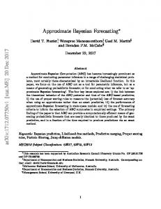
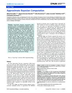
3 Two target scenarios We consider scenarios of two targets that maneuver in and out a formation flight. The corresponding 2D trajectory patterns are pictured in Figure 1 and in Figure 2. 4

2.5

x 10

2

1.5 1

1

0.5

0 2 -0.5

-1

0

0.5

1

1.5

2

2.5

3 4

x 10

Fig. 1. 2D trajectories from [14] 4

1.5

x 10

1 1

0.5

0

-0.5

-1 2 -1.5

-5000

0

5000

10000

15000

20000

Fig. 2. Trajectories of jointly maneuvering targets

The trajectory pattern in Figure 1 is from [14]. We refer to this as scenario R0. In addition to this we consider the jointly maneuvering target scenarios from [11], as depicted in Figure 2. Here, from 0 to 20s, targets 1 and 2 fly at a speed of 400 m/s in a straight line in south and north

11

NLR-TP-2006-736

direction respectively. From 20 to 35s, both targets make a coordinated turn to the east. From 35 s to 55s, both targets fly in a straight line to the east. From 55s to 70s, targets 1 and 2 make a coordinated turn to the north and to the south respectively. From 70s to 90s, targets 1 and 2 fly in a straight line to the north and to the south respectively. Of the jointly maneuvering target trajectories we consider seven scenarios, which differ in the initial position of Target 1 only: Scenario R1: Target 1 starts at (0,11820m) and target 2 starts at (0,-11820m). Scenario R2/R2’: Same as R1 but initial position of target 1 is shifted 200/100m to the south. Scenario R3/R3’: same as R1 but initial position of target 1 is shifted 200/100m to the north. Scenario R4/R4’: Same as R1 but initial position of target 1 is shifted 200/100m to the east. For each of the scenarios, Monte Carlo simulations containing 100 runs have been performed for each of the tracking filters. In order to make the comparisons more meaningful, for all tracking filters the same random number streams were used. For each of the tracking algorithms, we assume three possible modes, i.e. θ i ∈ {1, 2, 3} , with: Mode 1 (i.e. θ i =1): nearly constant velocity with zero mean perturbation in acceleration. The standard deviation of the process noise is σ ai (1) = 5m/s 2 . Mode 2 (i.e. θ i =2): Wiener process acceleration (nearly constant acceleration motion). The standard deviation of the process noise is σ ai (2) = 7.5m/s 2 . Mode 3 (i.e. θ i =3): Wiener process acceleration (with large acceleration increments, for the onset and termination of maneuvers). The standard deviation of the process noise is σ ai (3) = 40m /s 2 . The initial mode probabilities for each initial track are assumed to be: [0.8, 0.1, 0.1]. The mode switching probability matrix is assumed to satisfy equation (5.a) with: ⎡0.8 0.1 0.1⎤ Π = ⎢⎢ 0.1 0.8 0.1⎥⎥ , for i = 1,2. ⎢⎣ 0.1 0.1 0.8⎥⎦ i

We adopt this parameterisation in order to assure that none of the trackers uses any advantage of the fact that in scenarios R1/R1’ through R4/R4’ the targets start and stop maneuvering at the same moments in time. The target motion model used by the tracking algorithms is from [16]. In each mode the motion dynamics are modelled in Cartesian coordinates, where the state of the target is position, velocity and acceleration in each of the two Cartesian coordinates. Thus xti in (1) has dimension 2n = 6 , and the matrices a i (θ i ) and b i (θ i ) satisfy,

12

NLR-TP-2006-736

⎡ a i (θ i ) 0 ⎤ a i (θ i ) = ⎢ 1 ⎥, i a2 (θ i ) ⎦ ⎣ 0

⎡bi (θ i ) 0 ⎤ bi (θ i ) = ⎢ 1 ⎥ i b2 (θ i ) ⎦ ⎣ 0

⎡1 Ts i a j (1) = ⎢⎢0 1 ⎢⎣0 0

⎡ ⎢1 Ts ⎢ a ij (2) = a ij (3) = ⎢0 1 ⎢0 0 ⎢ ⎣

0⎤ 0 ⎥⎥ , 0 ⎥⎦

1 2⎤ Ts 2 ⎥ ⎥ Ts ⎥ 1 ⎥ ⎥ ⎦

1 bij (θ i ) = σ ai (θ i ) ⋅ Col{ Ts 2 , Ts , 0} . 2

The initial track state conditions used are: xˆ0i (θ i ) = x0i , θ i ∈ {1, 2,3}, i ∈ {1, 2} Pˆ (θ ) = Diag{Pˆ 1 (θ 1 ), Pˆ 2 (θ 2 )} 0

0

0

Pˆ0i (θ i ) = Diag{σ 12 , σ 2 (θ i ) 2 , σ 2 (θ i ) 2 }

with: σ 1 = 20 / 3, σ 2 (1) = 5 / 3, σ 2 (2) = 2.5, σ 2 (3) = 40 / 3 Both for the simulated measurements and the tracking filters, the potential sensor measurements for target i are assumed to satisfy equation (2) with the same coefficients for each θ i , i.e. ⎡ hi (θ i ) 0 ⎤ hi (θ i ) = ⎢ 1 ⎥, i h2 (θ i ) ⎦ ⎣ 0 hij (θ i ) = [1 0 0] ,

⎡ g i (θ i ) g i (θ i ) = ⎢ 1 ⎣ 0 g ij (θ i ) = σ m ,

⎤ ⎥ g (θ ) ⎦ 0

i 2

i

j ∈ {1, 2}

The standard deviation σ m of the measurement error is σ m = 20 m. The sensor is assumed to be located at the coordinate system origin. The sampling interval Ts = 1 s and the probability of detection Pd = 0.997 . False measurements are simulated at a high density of λ = 1×10−6 /m2 = 1/ km2 . The resolution parameter value is r1 = r2 = 10. The gates for setting up

the measurement validation regions are based on the threshold ν = 25 .

13

NLR-TP-2006-736

4 Monte Carlo simulations For scenarios R0-R4’, Monte Carlo simulations have been executed for the JIMMCPDA, JIMMCPDA*, JIMMCPDAR and JIMMCPDAR* filters (500 simulation runs per filter). We consider maintenance of confirmed tracks only, and no track initialisation, confirmation or termination. For each simulation run, we counted track i "O.K.", if hi xˆTi − h i xTi ≤ 9σ m

where | ⋅ | denotes the l2 -norm. We counted track i "Swapped", if track i is not "O.K." and hi xˆTi − h j xTj ≤ 9σ m

for j ≠ i .

We counted track i and j as "Coalescing Tracks" if at three or more consecutive observation moments: hi xti − h j xtj > 9σ m

∧

hi xˆti − h j xˆtj ≤ σ m

Using these criteria, the results of the Monte Carlo simulations for the scenarios are depicted in four Tables: •

The percentage of Both tracks "O.K.", in Table 1.

•

The percentage of Both tracks "O.K." or "Swapped", in Table 2.

•

The percentage of "Coalescing" tracks, in Table 3.

•

The average CPU time per scan in Table 4.

The results in Tables 1 and 2 show a significant impact of un-modelled sensor resolution on the tracking results for all scenarios, with the largest impact for scenarios where the two targets reach each other at 100m distance or less, i.e. R1 (0m), R2’ (100m), R3’ (100m) and R4’ (100m). Tables 1 through 3 show that JIMMCPDAR* performs much better than JIMMCPDA for all scenarios. The improved performance of JIMMCPDAR* over JIMMCPDA is partly caused by the track coalescence avoidance and partly by taking unresolved measurements into account. Moreover, by comparing the difference with the individual improvements of JIMMCPDA* and JIMMCPDAR over JIMMCPDA, it becomes clear that the two enhancements show to enforce each other for the most demanding scenarios (R1, R2’, R3’ and R4’).

14

NLR-TP-2006-736

Table 1 also show that both tracks ‘O.K.’ performance of all four filters varies significantly with the geometry of how aircraft maneuver in and out a formation flight. JIMMCPDAR* performance varies least to these variations. We also investigated if the novel filters could perform well in case of perfect sensor resolution scenarios. The results of these Monte Carlo simulations are given in Tables 5 through 7. As expected, JIMMCPDA and JIMMCPDA* are now doing much better than in Tables 1 through 3. However, JIMMCPDAR and JIMMCPDAR* also perform significantly better on the perfect resolution scenarios than on the scenarios with unresolved measurements.

Table 1 % Both tracks ‘O.K.’

Scenario

JIMMCPDA

JIMMCPDA* JIMMCPDAR JIMMCPDAR*

R0

94.0

94.2

99.2

99.2

R1

0.0

0.0

1.6

11.8

R2

27.4

34.2

28.4

40.2

R2’

0.6

0.2

1.8

31.6

R3

57.2

70.6

65.2

81.4

R3’

1.6

2.4

3.0

40.4

R4

51.8

72.4

63.4

89.4

R4’

0.8

1.6

1.6

42.0

Table 2 % Both tracks ‘O.K.’ or both tracks ‘Swapped’

Scenario

JIMMCPDA

JIMMCPDA* JIMMCPDAR JIMMCPDAR*

R0

94.0

94.2

99.2

99.2

R1

0.0

0.2

3.8

32.0

R2

53.8

69.0

64.8

96.8

R2’

0.8

0.4

3.4

72.2

R3

81.2

89.6

87.2

98.4

R3’

3.0

4.8

9.4

81.6

R4

78.0

89.8

86.2

99.0

R4’

1.4

3.2

3.2

79.8

15

NLR-TP-2006-736

Table 3 % Coalescing tracks

Scenario

JIMMCPDA

JIMMCPDA* JIMMCPDAR JIMMCPDAR*

R0

0.0

0.0

0.0

0.0

R1

0.0

0.0

36.8

0.2

R2

17.8

0.2

38.0

0.6

R2’

1.0

0.0

76.0

0.0

R3

15.6

0.4

19.8

0.2

R3’

3.8

0.0

73.8

0.0

R4

15.2

0.2

16.6

0.2

R4’

1.4

0.0

82.6

0.0

Table 4 Average CPU time per scan (in milliseconds)

Scenario

JIMMCPDA

JIMMCPDA* JIMMCPDAR JIMMCPDAR*

R0

265

250

361

362

R1

638

620

625

521

R2

375

329

449

342

R2’

638

601

553

411

R3

275

236

378

336

R3’

607

598

525

365

R4

291

226

372

335

R4’

625

608

549

384

Table 5 % Both tracks ‘O.K.’ under Perfect Resolution (PR)

Scenario

JIMMCPDA

JIMMCPDA* JIMMCPDAR JIMMCPDAR*

R0

99.0

99.0

98.8

98.8

R1

0.6

55.0

1.0

53.2

R2

80.6

82.2

72.8

72.2

R2’

9.6

43.8

7.4

43.4

R3

94.6

97.8

91.2

97.2

R3’

6.6

31.2

5.4

27.2

R4

96.6

98.2

94.8

97.6

R4’

12.4

82.2

10.2

82.2

16

NLR-TP-2006-736

Table 6 % Both tracks ‘O.K.’ or both tracks ‘Swapped’ under PR

Scenario

JIMMCPDA

JIMMCPDA* JIMMCPDAR JIMMCPDAR*

R0

99.0

99.0

98.8

98.8

R1

1.0

99.2

1.2

98.8

R2

96.4

99.0

94.4

99.2

R2’

24.8

99.0

16.4

98.2

R3

96.6

99.2

95.4

99.2

R3’

26.6

99.2

21.8

99.2

R4

97.0

98.2

97.0

98.2

R4’

18.6

98.6

15.6

98.4

Table 7 % Coalescing tracks under Perfect Resolution

Scenario

JIMMCPDA

JIMMCPDA* JIMMCPDAR JIMMCPDAR*

R0

0.0

0

0.0

0

R1

99.8

0

99.8

0

R2

1.6

0

3.0

0

R2’

49.8

0

61.6

0

R3

4.6

0

6.8

0

R3’

55.2

0

58.4

0

R4

1.2

0

1.2

0

R4’

69.4

0

76.4

0

The results show that the two imperfect resolution filters which are based on the measurement model of [5] are far less sensitive to a difference between resolution model and reality than the two perfect resolution filter versions are. This confirms the expected robustness of the resolution model of [5]. Table 4 shows that the average computational load is quite similar for all four filters, and even with best average values for JIMMCPDAR*.

17

NLR-TP-2006-736

5 Conclusion We evaluated four approximate Bayesian filters that have been developed over a series of studies [9]-[12]. The baseline algorithm JIMMCPDA uses a Joint IMM for the joint maneuver modes of the two targets, in combination with an enhanced version of JPDA that takes the coupling between target state estimates into account. The other three JIMMCPDA*, JIMMCPDAR and JIMMCPDAR* have been developed as further enhancements over this baseline algorithm. JIMMCPDA*’s enhancement is track coalescence avoidance, JIMMCPDAR’s enhancement is taking unresolved measurements into account, and JIMMCPDAR* incorporates both enhancements. Monte Carlo simulation results of these four filters for the considered example of tracking two targets that maneuver in and out formation flight, show a significant advantage of the filter which takes both limited resolution and track coalescence avoidance into account. This corroborates the argumentation by [1], [2] about the high relevance of limited sensor resolution. It also shows that the resolution model of [5] allows the filters to keep on performing well in case the true sensor resolution is better than assumed. Hence, for the considered example of tracking two targets that maneuver in and out a formation flight amidst unresolved, missing and false measurements, the JIMMCPDAR* filter is the absolute winner, whereas JIMMCPDA* and JIMMCPDAR perform second best and JIMMCPDA performs least. The nice results obtained with the JIMMCPDAR* filter for two targets forms a strong motivation to extend the approach to more than two targets. Follow-up research of complementary interest is to compare the performance of the novel filters with those of a good particle filter approximation of the exact recursive Bayesian filter.

18

NLR-TP-2006-736

References [1] F.E. Daum, A system approach to multiple target tracking, Ed: Y. Bar-Shalom, Multitarget-Multisensor Tracking, Volume II, Artech House, 1992, pp. 149-181. [2] F.E. Daum, R.J. Fitzgerald, The importance of resolution in multiple target tracking, Proc. SPIE Signal&Data Processing of Small Targets, Vol. 2238, 1994, pp. 329-338. [3] K.C. Chang, Y. Bar-Shalom, Joint Probabilistic Data Association for multitarget tracking with possibly unresolved measurements and maneuvers, IEEE Tr. Automatic Control, Vol. 29 (1984), pp. 585-594. [4] S. Mori et al., Tracking aircraft by acoustic sensors – multiple hypothesis approach applied to possibly unresolved measurements, Proc. ACC, 1987, pp. 1099-1105. [5] W. Koch, G. Van Keuk, Multiple hypothesis track maintenance with possibly unresolved measurements, IEEE Tr. AES, Vol. 33 (1997), pp. 883-892. [6] W. Koch, On Bayesian MHT for formations with possibly unresolved measurements – Quantitative results, Proc. SPIE, Signal and Data Processing of Small Targets, 1997, Vol. 3163, pp. 417-428. [7] W. Koch, Experimental results on Bayesian MHT for maneuvering closely-spaced objects in a densely cluttered environment, Proc. RADAR1997, IEE, 1997, pp. 729-733. [8] D.J. Salmond, N.J. Gordon, Group tracking with limited sensor resolution and finite field of view, Proc. SPIE Signal & Data Proc. of Small Targets, 2000, Vol. 4048, pp. 532-540. [9] H.A.P. Blom, E.A. Bloem, Tracking multiple maneuvering targets by Joint combinations of IMM and PDA, Proc. 42nd IEEE CDC, Mauii, December 2003, pp. 2965-2970. [10] H.A.P. Blom, E.A. Bloem, Exact Bayesian filter and joint IMM coupled PDA tracking of maneuvering targets from possibly missing and false measurements, Automatica, Vol. 42 (2006), pp. 127-135 and p. 887. [11] H.A.P. Blom, E.A. Bloem, Joint IMM and Coupled PDA to track closely spaced targets and to avoid track coalescence, Proc. 7th Int. Conf. on Information Fusion, July 2004, Stockholm, pp. 130-137. [12] H.A.P. Blom, E.A. Bloem, Tracking multiple maneuvering targets from possibly unresolved, missing or false measurements, Proc. 7th Int. Conf. on Information Fusion, Philadelphia, July 25-29, 2005. [13] J.K. Tugnait, Tracking of multiple maneuvering targets in clutter using multiple sensors, IMM and JPDA Coupled Filtering, IEEE Tr. AES, Vol. 40 (2004), pp. 320-330. [14] B. Chen, and J. K. Tugnait, “Tracking of multiple maneuvering targets in clutter using IMM/JPDA filtering and fixed-lag smoothing,” Automatica, vol. 37 (2001), pp. 239-249.

19

NLR-TP-2006-736

[15] H.A.P. Blom, E.A. Bloem, Bayesian tracking of two possibly unresolved maneuvering targets, IEEE Tr. AES, appears 2007. [16] A. Houles, Y. Bar-Shalom, Multisensor tracking of a maneuvering target in clutter, IEEE Tr. AES, Vol. 25 (1989), pp. 176-188.

20

NLR-TP-2006-736

Appendix A Acronyms CPDA

Coupled PDA

CPDA*

Track-coalescence-avoiding CPDA

IMM

Interacting Multiple Model

IMMJPDA

Interacting Multiple Model Joint Probabilistic Data Association

IMMJPDA*

Track-coalescence-avoiding IMMJPDA

IMMPDA

Interacting Multiple Model Probabilistic Data Association

JIMMCPDA

Joint Interacting Multiple Model Coupled Probabilistic Data Association

JIMMCPDA*

Track-coalescence-avoiding JIMMCPDA

JIMMCPDAR

JIMMCPDA with Resolution

JIMMCPDAR*

Track-coalescence-avoiding JIMMCPDAR

JPDA

Joint PDA

JPDA*

Track-coalescence-avoiding JPDA

MHT

Multiple Hypotheses Tracking

PDA

Probabilistic Data Association

21

NLR-TP-2006-736

Appendix B List of Symbols a i (θ i )

Target i’s state transition matrix of size n × n as a function of mode θ i

A(θ ) b (θ )

Joint targets state transition matrix as a function of joint mode θ Target i’s state noise gain matrix of size n × n′ as a function of mode θ i

B(θ )

Joint targets state noise gain matrix as a function of joint mode θ

Dt

Total number of detected targets at moment t

ft

Column vector of Ft i.i.d. false measurements

Ft

Total number of false measurements at moment t

φi ,t φt

Detection indicator for target i at moment t

i

i

Detection indicator vector at moment t, containing the detection indicators for all targets at moment t

Φ

g (θ ) i

i

Matrix operator to link the detection indicator vector with the measurement model Target i’s measurement noise gain matrix of size m × m′ as a function of mode θ i

G (θ ) χ% t

Joint targets measurement noise gain matrix as a function of joint mode θ (0,1)-matrix that is used to randomly select target measurements from the

χ% t

measurement vector yt “Inflated” χ% t matrix of proper size such that it randomly selects target measurements from the measurement vector yt by means of matrix multiplication.

h (θ ) i

i

Target i’s state-to-measurement transition matrix of size m × n as a function of mode

θi H (θ )

Joint targets state-to-measurement transition matrix as a function of joint mode θ

I

Unit-matrix

Ir

Diagonal matrix with its i-th diagonal equal to the i-th element of the vector r

κt

Merging indicator at moment t

Lt

The number of measurements at moment t

λ

Spatial density of false measurements

M

Total number of targets

M

Set of possible modes of target

N

Total number of modes of a target

ν

Measurements gate threshold i d

P

Detection probability of target i

Πηθ

Transition probability of a target switching from mode η to mode θ

Π

Transition probability matrix

ψ i.t ψt

Target indicator for measurement i at moment t Target indicator vector at moment t, containing the target indicators for all measurements at moment t

22

NLR-TP-2006-736

ri

Resolution capability factor for the i-th noise component of a potential target measurement

R(θ )

Resolution capability matrix of size m × m

σ (θ ) σm θti θt i a

i

Target i’s system noise standard deviation as a function of mode θ i Measurement noise standard deviation Mode of target i at moment t Joint targets mode at moment t Sequence of i.i.d. standard Gaussian variables of dimension m′ representing the

i t

v

measurement noise for target i Joint targets measurement noise vector

vt

Volume of the observed region

V i t

w

Sequence of i.i.d. standard Gaussian variables of dimension n′ representing the system noise for target i

wt

Joint targets system noise vector

xti

n-vectorial state of target i at moment t

xt

Joint targets state vector at moment t

k t

y

k-th measurement at moment t

yt

Measurement vector at moment t, containing all measurements at moment t

Yt

σ -algebra generated by measurements up to and including moment t

i t

z

m-vectorial potential measurement of target i at moment t

zt

Joint measurements vector at moment t, containing the potential measurements of all targets at moment t

z%t

Joint measurements vector at moment t, containing the potential measurements of all detected targets at moment t in a fixed order

23