Bayesian methods for visual tracking model the likelihood of image measurements ..... It is important to mention several key properties that make Gibbs learning ...
Gibbs Likelihoods for Bayesian Tracking Stefan Roth Leonid Sigal Michael J. Black Department of Computer Science, Brown University Providence, RI, USA 02912 {roth,ls,black}@cs.brown.edu
Abstract Bayesian methods for visual tracking model the likelihood of image measurements conditioned on a tracking hypothesis. Image measurements may, for example, correspond to various filter responses at multiple scales and orientations. Most tracking approaches exploit ad hoc likelihood models while those that exploit more rigorous, learned, models often make unrealistic assumptions about the underlying probabilistic model. Such assumptions cause problems for Bayesian inference when an unsound likelihood is combined with an a priori probability distribution. Errors in modeling the likelihood can lead to brittle tracking results, particularly when using non-parametric inference techniques such as particle filtering. We show how assumptions of conditional independence of filter responses are violated in common tracking scenarios, lead to incorrect likelihood models, and cause problems for Bayesian inference. We address the problem of modeling more principled likelihoods using Gibbs learning. The learned models are compared with na¨ıve Bayes methods which assume conditional independence of the filter responses. We show how these Gibbs models can be used as an effective image likelihood, and demonstrate them in the context of particle filter-based human tracking.
1. Introduction We develop an image likelihood model for visual tracking that represents conditional dependencies between various image cues at multiple scales. Likelihoods are learned from a novel training set of human motion imagery in which we have “ground truth” human poses in video sequences; the method, however, is applicable to any tracking scenario for which training data is available. Likelihoods are represented by a Gibbs model [8, 19], which is based on the maximum entropy principle and learned from the training data. The approach extends previous work on modeling natural image statistics and applies this to the problem of Bayesian tracking. Tracking can be viewed as a problem of probabilistic inference from ambiguous sensor measurements. Recent approaches adopt a Bayesian formulation in which local im-
2
1
1
2
3
1
4
1
2
3
4
1
2
3
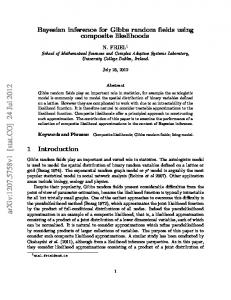
Figure 1: Learning Gibbs distributions from marginals. The log-histogram of the empirical 2D distribution in the center shows the joint statistics of first derivative filter responses at two adjacent scales conditioned on the pose of a human arm. The marginal (log) histograms are taken along the directions marked by dashed white lines; these correspond to the x- and y-axes, as well as the two diagonals. As we use more marginals to approximate the joint, the approximation improves (clockwise from upper left). The na¨ıve Bayes model corresponds to the product of the x and y marginals (upper right). Our full Gibbs model exploits all four marginals (lower left).
age measurements are combined with a priori information to derive an a posteriori density estimate over the tracking hypotheses. The quality of any Bayesian solution is only as good as the local evidence (likelihood) and prior models. Many Bayesian tracking approaches adopt ad hoc likelihoods or make strong simplifying assumptions about the conditional independence of image measurements. We demonstrate how such assumptions lead to incorrect likelihood models and how this, in turn, leads to brittle tracking in a particle filter framework. Let x be a vector of parameters representing the state of the object being tracked and let f = [f1 , . . . , fn ]T be a vector of image measurements1 . Here we take the fi to be 1 “Images”
may be grayscale images, stereo depth maps, silhouettes, or any other sensor measurement. The filters could be identity functions that return the original measurements or any other linear (or non-linear) filter. Regardless, the likelihood modeling problem remains the same.
various filters (first and second derivatives of Gaussians at multiple scales) at image locations and orientations determined by the object state. In its simplest form, the Bayesian framework involves estimating p(x | f ) ∝ p(f | x) p(x). Our goal is to model the likelihood, p(f | x), of observing the filter responses f conditioned on the state x. Consider the empirical joint conditional density in Figure 1 (center), which shows a distribution of filter responses on the boundary of human limbs. The axes correspond to first derivative filter responses at two adjacent image scales conditioned on the known limb orientation. A common assumption is that the filter responses are conditionally independent across scale and consequently the joint probability can be approximated by the product of the marginal probabilities at Q each scale ((1) and (2) in the figure); that is, p(f | x) = i p(fi | x). This corresponds to a na¨ıve Bayes assumption. The product of marginals is shown in Figure 1 (upper right). While the marginals for this and the center plot are the same, the joint conditional density is very different. Modeling the full joint conditional density is difficult because: (1) filter responses and other image measurements are typically non-Gaussian; (2) many features or measurements are required for robust tracking which makes the dimensionality of the joint space high; (3) there may be significant dependencies between measurements that make simple independence assumptions inappropriate; and (4) training data may be too limited to fully populate a highdimensional joint probability space. To address these problems we model the likelihood using a Gibbs model ! X 1 (i) (i) hλ , φ (f , x)i , exp − p(f | x) = Z(Λ) i where the λ(i) are weight functions that we must learn and the φ(i) can be thought of as “selector” functions that choose bins of marginal histograms along various directions in the filter space. The partition function, Z(Λ), acts as a normalization term. Here the φ(i) select both histograms for individual filter types as well as histograms for combinations of two filters (e.g. across adjacent scales). An example of learning such a Gibbs model with four marginals is shown in Figure 1 (lower left). A general method for learning such Gibbs models was presented by Zhu and Mumford [18]. The key idea is to learn the λ(i) such that the marginal statistics of the Gibbs model match the marginal statistics that we can easily compute from training data. Note that the learning algorithm can match marginals along arbitrary directions in the parameter space [8]. We exploit a simplified version of the
algorithm in [8] and marginalize along fixed directions “between” pairs of filter responses. Regardless of the dimensionality of the joint space, we need only model marginals. This reduces the amount of training data needed to avoid overfitting. The model also imposes a maximum entropy condition which ensures that the learned model makes the least commitment in areas where it is not constrained by the marginals. Proper probabilistic models are critical for Bayesian tracking. We show that na¨ıve Bayes methods can overestimate the likelihood resulting in overly sharp peaks in the likelihood distribution. Such peaks are particularly problematic for Monte Carlo sampling methods such as particle filtering. We demonstrate how Gibbs models produce better approximations to image likelihoods and consequently result in more reliable tracking in a particle filtering framework. We show how they can be used to model the likelihood of human limbs and that the resulting models are less distracted by clutter than na¨ıve Bayes models.
1.1. Other related work A complete review of image likelihoods used in Bayesian tracking is beyond the scope of this paper. We focus, instead, on human motion tracking and, in particular, the use of linear filters as image measurements. The marginal statistics of filter responses in natural images have received a great deal of attention [9, 11, 14, 19] and it has often been noted that these marginals are strongly non-Gaussian with heavy tails. It has also been noted that wavelet filter responses are statistically dependent across scale and across different filter types [9, 14]. In [12] the marginal statistics of first and second derivative responses at multiple scales were used to model the likelihood of human limbs for 3D person tracking. We take a similar approach and exploit a novel set of training data containing synchronized video imagery and 3D “ground truth” human motion [13]. Given the known limb pose we steer the filter responses to the limb orientation and compute the statistics for first derivative filters along and across the limb edges as well as for second derivative filters in the center of the limb (at an appropriate scale [12]). In [12] the marginal probabilities of filter responses were multiplied in a na¨ıve Bayesian model. There have been many uses of filter responses for Bayesian tracking and some of these have attempted to reduce conditional dependence by spacing filters sufficiently far apart [6, 10, 15, 16]. These methods are approximate and do not attempt to learn any remaining conditional dependence. Here we show that the filter responses on human limbs are conditionally dependent, and we approximate the joint conditional density with a Gibbs model. We focus on exponential models of the likelihood and take the Gibbs learning approach [18]. There are many re-
0
0
0
−5
−5
−5
−10 0
Figure 2: Training Data. Example frames from the training set used to learn human limb likelihoods. The 3D body model is obtained by a commercial motion capture system and is projected into four calibrated camera views. This gives the known position and orientation of the limbs in each view.
lated learning approaches in the literature such as projection pursuit density estimation [2, 17], and products of experts [4]. We are unaware of previous uses of Gibbs learning for likelihood modeling and Bayesian detection and tracking.
a
−10
0
50
b
0
50
c
Figure 3: Marginal statistics of first derivative filter responses. All plots show log-histograms. (a) Empirical distribution at 3 scales for the filter response orthogonal to the limb boundary (fe ). (b) Distribution for the filter response aligned with the limb (fl ). (c) Filter response in the background.
specifically, the image response for an edge of orientation θ at pyramid level σ and position y is formulated as the image gradient perpendicular to the edge orientation θ: fe(σ) (y, θ) = sin θ fx(σ) (y) − cos θ fy(σ) (y)
2. Image Statistics Image derivatives have proven to be useful cues for modeling edges. To illustrate the use of Gibbs models for tracking, we consider the case of tracking human limbs. We formulate two conditional likelihood models, pFG (f |x) for the foreground and pBG (f |x) for the background2. These models describe the likelihood of observing a limb in terms of the likelihood ratio pR (f | x) ∝
−10 50
pFG (f | x) . pBG (f | x)
(1)
Although our discussion focuses on human tracking, the model can be generalized to other objects.
2.1. Training data In many 3D human tracking applications limbs are modeled as tapered cylinders, so that the edges of the projected cylinder coincide with the intensity edges of limbs in the observation. Our training data set (see Figure 2) consists of 4000 images (1000 frames from 4 different views each) of a person in normal clothes walking in a laboratory environment. Along with the video images we have ground truth data of such a body model indicating the 3D position and orientation of the subjects’ limbs [13]3 . To obtain filter responses at various spatial scales, we construct a Gaussian pyramid with levels σ = 0, . . . , 2 (0 is the original image). At each scale σ we compute the first (σ) (σ) derivatives, [fx , fy ], of the image brightness function in the horizontal and vertical directions at various locations along the projected edge. Since we are interested in filter responses conditioned on the limb orientation, we steer the filter responses to that orientation as suggested in [12]. More 2 When our discussion applies to both the foreground and the background model, we will drop the subscript. 3 Data available at http://www.cs.brown.edu/research/vision/motioncapture/.
(2)
We will refer to the first derivative at scale σ along the edge (σ) (σ) (i.e. orthogonal to fe ) as fl . Figure 3 shows examples of steered edge responses for a lower arm at different pyramid levels. As in [12], we compute the second derivative across the edge fr and along the edge frl at a scale σ that is chosen so that the filters capture the ridge character of the whole limb. The second derivative filters are evaluated at locations on the mid line between the two sides of the limb. The response is steered to the limb orientation similar to eq. (2) (see [12] for details). The training data for the background model is acquired in essentially the same way. We compute the same filter responses at arbitrary locations and orientations in the views of the same scene, but with the person absent. In contrast to [6] this is a generic background model. If we compute image derivatives at nearby locations along the edges of the limb, the responses of a particular filter will be strongly dependent between spatial locations, especially at coarser scales. Here we make the simplifying assumption that the filter responses along the edge are fully dependent along each side or the mid line respectively4. For simplicity of exposition, we consider only the absolute value of the derivatives. Furthermore, we capture the statistics of both sides of the limb in a single model. Our filter bank finally becomes h i (0) (1) (2) f = |fe(0) |, |fe(1) |, |fe(2) |, |fl |, |fl |, |fl |, |fr |, |frl | .
2.2. Marginal densities Figure 3 shows a few examples of marginal histograms from the training data. The left two plots show the log-histograms 4 The Gibbs model we use would be capable of jointly modeling the responses of the various locations along the edge, but we leave this for future work.
of the absolute response of derivative filters steered according to the edge orientation, either across or along the edge. As expected, the responses at all scales and in both orientations are non-Gaussian. Moreover, the filter responses are fairly consistent across scale. If we compare the histograms for the derivatives across and along the edge, we immediately see that the filter response histogram for fe is more heavy-tailed than the histogram for fl . This intuitively makes sense, because we expect large derivatives to occur across the edge, but not so much along the edge. We also observe that the maximum of the histogram occurs at or near zero, which is due to indistinct limb edges that are common in real images [12]. The derivative across the edge at the finest scale is less heavy-tailed than at the two coarser scales. This is due to our simple limb model, which assumes the edges of the limb to be straight. At coarse scales the edge is more likely to fall within the scope of the filter response. Comparing these histograms to the background distribution, we see that the background tends to contain large gradients as well. Since their orientation does not necessarily coincide with limb orientations, the broadness of the distribution is somewhere between the broadness of the two edge histograms. Here as well, the filter response statistics are consistent across scale.
2.3. Joint densities The majority of work on visual tracking has assumed that image measurements are conditionally independent given the body pose. On the other hand, it is known that image filter responses (wavelets, derivatives of Gaussians, etc.) are not statistically independent. As noted by Simoncelli [14], conditional histograms of filter responses at neighboring scales or neighboring locations exhibit strong dependence. This is true even when carefully selected filters decorrelate the data. For simplicity, we focus here on conditional dependence across scale and between different types of filters. The same analysis applies to spatial dependence, which can be dealt with in a similar manner. Knowing the limb orientation does not tell us the edge contrast or even whether there is any observable edge in the image. Conditional dependence exists here because whatever image structure is present tends to be consistent across scale. This is illustrated in Figure 1 where the empirical joint density is plotted for fe at 2 scales (center). We can clearly see that joint steered responses across scales are not conditionally independent, because the probability mass extends on a ridge along the diagonal. In the upper right we show the effect of approximating this distribution by the product of the marginals. The so-called na¨ıve Bayes model hence treats p(fe(1) , fe(2) | x) = p(fe(1) | x)p(fe(2) | x) .
0
0
0
−10
−10
−10
−20 0
20
a
−20 0
20
−20 0
b
20
c
Figure 4: Learned λ weight functions in the Gibbs likelihood (1) (1) model. (a) λ for fe (solid) and fl (dashed) (b) same for scale (2) (2) (1) (1) 2 (c) λ for 12 (fe + fe ) (solid) and 12 (fe − fe ) (dashed). As we can see this assumption leads to a poor representation of the actual joint. The result captures the non-Gaussian nature of the statistics (high kurtosis) but not its skewness. From Figure 7 we can see that the first and second derivatives across the edge show conditional dependence as well. Our conclusion is that simple models that are based on products of marginals fail to capture important properties of the joint distribution of filter responses conditioned on the edge orientation5.
3. Gibbs Likelihood Models Gibbs models have appeared in the computer vision literature in various guises, for example in the form of Markov random fields. Zhu et al. [19] were among the first to formally introduce a more general framework for Gibbs learning. There is an extensive literature to which we refer the reader for more technical detail [8, 18, 19]. It is important to mention several key properties that make Gibbs learning attractive: As already mentioned in the introduction, Gibbs learning is based on the principle of learning a probability distribution from a number of its marginals. Using marginal statistics has the advantage that fairly little training data is needed to learn the distribution. Furthermore, Gibbs distributions have the property that they are maximally smooth in areas where they are not constrained by the marginals. Again, this avoids overfitting and leads to the learning algorithm being fairly insensitive to having small amounts of training data. Although learning a Gibbs model is computationally intensive, evaluating such a log-linear model is very fast. Gibbs models arise from a few, quite simple, axioms: 1. The learned distribution p(f | x) should preserve select marginal statistics of the distribution to be learned: Let φ(i) (f , x) be a set of typically real- or vector-valued functions6 of the filter responses f , and let µ(i) be 5 While taking the product of marginals along other directions might alleviate this problem somewhat, the resulting joint nevertheless fails to model, for example, the slightly “bent” character of the ridge in Figure 1, which can be in fact modeled using a full Gibbs model. 6 Continuous interpretations exist where the function values φ(i) (f , x) are functions themselves. Since they don’t differ from the discrete case very much, we omit them here for brevity.
0
0
−5
−5
−10 0 0
−10 10
20
30
0 0
−5
−5
−10
−10
0
10
20
30
0
10
20
30
there is a simple iterative scheme that is guaranteed to converge. If at time step n we have a Gibbs distribution ! X (i) (i) hλn , φ (f , x)i , pn (f | x) ∝ exp − i
then we update the weights using (see [8]) h i (i) (i) (i) λn+1 = λ(i) + α log(µ ) − log E [φ (f , x)] . p (f | x) n n
10
20
30
Figure 5: Log-marginals of the foreground data for the lower left leg (green with circles), as well as na¨ıve Bayes (red with crosses) and Gibbs (blue) fits. (Top row) From left to right: (2) (1) Across edge on first scale p(fe ) and second scale p(fe ). (Bot(2) (1) 1 tom row) From left to right: Average response p( 2 (fe + fe )) (2) (1) 1 and difference of responses p( 2 (fe − fe )). their (empirical) expectations over the training data. In the case considered here, the µ(i) are 1D marginal histograms. The concept of preserving the empirical marginals can be written as h i Ep(f | x) φ(i) (f , x) = µ(i) , ∀i. (3) 2. Furthermore, we require the distribution to be maximally uninformative (i.e. “smooth”), subject to these constraints. This is achieved by requiring the learned distribution p(f | x) to have maximal entropy. We formulate this as a search problem over all distributions p(f | x): Z maximize − p(f | x) log(p(f | x)) df (4) h i s.t. Ep(f | x) φ(i) (f , x) = µ(i) , ∀i. It can be shown that the solution to this entropy maximization problem under the given marginal constraints has the form of a Gibbs distribution: ! X hλ(i) , φ(i) (f , x)i , (5) p(f | x) ∝ exp − i
where h·, ·i is either a product of scalars, or the Euclidean scalar-product. The λ(i) can be thought of as weight functions for each marginal. In our discrete realization, these weights are vectors. We are not aware of an intuitive interpretation of the exact shape of these weight functions, except for special cases (see below). Figure 4 shows examples of various λ weight functions for the learned likelihood model. The question remains, how the weights λ(i) can be chosen in order to satisfy the marginal constraints. Fortunately,
The marginals of pn (f , x) are computed using Monte-Carlo integration. The simplest version involves a standard Gibbs sampler [19], and more advanced importance samplingbased techniques have been proposed [8]. In our implementation the domain of the probability distribution is fairly low-dimensional, so we chose a Gibbs sampler for simplicity, which is sufficiently fast; the algorithm runs in at most a few minutes with good accuracy. While we take the φ(i) (f , x) to select 1D marginal histograms, the theory admits more general functions. Assume for simplicity that each filter response is an integer in {1, . . . , N }. We chose to discretize the filter responses into 32 bins. Then the “selector” function φ(f , x)(i) = ej ⇔ fi = j selects histogram bin j of the i-th component of f . In other words, the j-th component of φ is 1 when filter response fi falls into histogram bin j; the other components are 0. If we take the expectation over this φ function, then we obtain the marginal histogram of fi . If we have exactly one such φ function per component of f , then the Gibbs model is equivalent to the na¨ıve Bayes model, because each component of f is modeled independently of the others and its marginal statistics are identical to the empirical marginals. In this special case the weights λ(i) are proportional to the negative logarithm of the respective empirical marginal. However, the generality of the Gibbs model allows us to go beyond this. We can consider selector functions such as φ(f , x) = ej ⇔ 21 (f1 + f2 ) = j, which captures the statistics of the average of f1 and f2 . We should note that the combination of filter responses defining this φ is no longer orthogonal to the ones we previously considered, which is exactly the reason why we can model more complex properties of the joint. In this case the weights λ(i) have to correct for the fact that the joint Gibbs distribution is no longer simply a product of marginals. More generally, we can use marginal histograms along any line in the space of filter responses to model the joint. We can express this (again in a discretized way) as φ(f , x) = ej ⇔ dT f = j, where d is some marginal direction. Due to the quite simple filter bank considered here, we have a good intuition for the dependencies between the random variables. Hence it is possible to choose marginal directions by hand to capture the properties that one wishes to model. We choose the marginals of the individual filter responses, as well as diagonal marginals (average and
0
0
−5
−5
−10 0 0
−10 10
20
30
0 0
−5
−5
−10
−10
0
10
20
30
0
10
20
30
10
20
30
Figure 6: Log-marginals of the background data (green with circles), as well as na¨ıve Bayes (red with crosses) and Gibbs (blue) fits. (Top row) From left to right: Across edge on first scale (2) (1) p(fe ) and second scale p(fe ). (Bottom row) From left to (2) (1) 1 right: Average response p( 2 (fe + fe )) and difference of re(2) (1) 1 sponses p( 2 (fe − fe )).
difference) between filter responses across scale and between the first and second derivative. Alternatively, one can employ methods for automatically selecting important marginals [8, 19].
4. Experimental Results The experiments here are designed to illustrate properties of the Gibbs likelihood in Bayesian tracking scenarios. We focus on simple tracking and detection experiments where we can clearly attribute the change in performance to the better likelihood model. From Figures 5 and 6 we see that the marginals of the data, taken along the chosen directions, are essentially identical to the marginals of the learned Gibbs distribution. As we also expected, the marginals of the na¨ıve Bayes model coincide with the marginals of the data only for single derivative responses. However, the plots of the marginals along a diagonal in the filter space, which represent some combination of filter responses, show that the na¨ıve model fails to capture important properties of the joint distribution. Observing large filter responses that are consistent across scale is much less likely in the na¨ıve model than it should be given the training data. This is true for both the foreground model, as well as the background model. The 2D marginals in Figure 7 show that the Gibbs model qualitatively approximates the joint conditional likelihood better than the na¨ıve model. For quantitative comparison, Model Foreground Background
Gibbs na¨ıve Gibbs na¨ıve
Training data -6.21 -7.68 -4.90 -5.72
Test data -5.56 -6.77 -4.06 -4.59
Table 1: Average log-likelihood of the data sets in the Gibbs and na¨ıve Bayes models.
Figure 7: 2D log-marginals. The top row shows the histograms of the foreground data for the lower left leg (left two columns) and the background data (right two columns). The middle row shows the Gibbs model and the bottom row the na¨ıve Bayes fit. The 1st and 3rd column show the joint derivative filter responses between (2) (1) scale 1 and scale 2; i.e. p(fe , fe ). The 2nd and 4th column (2) show the joint of first and second derivative filters, p(fe , fr ).
we computed the average log-likelihood for the training data and test data for both foreground and background models. The test data consisted of 700 other frames captured the same way as the training data. Table 1 shows that the Gibbs models fit the training data significantly better than simple products of marginals. Also, the log-likelihoods of the test data are of the same magnitude as on the training data, from which we can conclude that we did not overfit the distributions. In an experiment relevant to human tracking, we shift the model of a human leg across the image orthogonal to the leg’s orientation. Here, the parameters x are the limb’s position and orientation. At each limb location we evaluated the log-likelihood ratio (see eq. (1)) of foreground to background at 15 points along each side of the limb. We averaged the log-likelihood ratios over all points along the limb, which is consistent with our assumption of full conditional dependence between spatial locations. Figure 8 illustrates how the log-likelihood ratio of the two models varies as we shift the model. For comparison purposes, we implemented an estimator of the ground truth likelihood based on a nearest neighbor approach 7. As we can see, the ground truth as well as the two models show local maxima near the actual limb position around 0 (this position was manually selected). We notice that the Gibbs model approximates the ground truth log-likelihood ratio well. The na¨ıve model shows local maxima in the right place, however it “overshoots” and makes the foreground more likely than it is given our training data. While this may not seem like a disadvantage (e.g. for maximum likelihood estimation) this 7 We should note that such a non-parametric “ground truth model” is only feasible when there is an abundance of training data available. But even then, the computation quickly becomes infeasible.
8
12 6
10 4
8
2
6
0
4
−2
2
−4 −40
−20
0
20
40
Figure 8: Log-likelihood ratio between foreground and background models for a lower leg. The ground truth is shown in green (with circle markers), the na¨ıve Bayes model in red (with crosses), and the full Gibbs model in blue.
overshooting has severe drawbacks for Bayesian tracking as discussed next.
4.1. Particle filtering Particle filtering [3, 5] provides a simple and popular method for Bayesian tracking with general (non-Gaussian) likelihoods. The problem of sample impoverishment is well known [7] and causes particle filters to reliably loose track when the posterior is multi-modal. Such tracking failures are often traced to the likelihood and, moreover, to the presence of a few peaks in the likelihood that attract all the samples. It is not uncommon to find likelihoods under which a single sample is several orders of magnitude more likely than all the others; in such cases, Monte Carlo sampling fails to capture the “true” posterior. A number of ad hoc methods have been exploited to tame the peaks in the likelihood. These typically correspond to “smoothing” the likelihood by raising it to some fractional power. For example, annealed particle filtering [1] exploits this idea to gradually introduce the influence of the peaks by changing the smoothing parameter. The true problem is not how to deal with these peaks computationally but rather that they are often due to a failure of the likelihood model. In particular, they can be caused by a na¨ıve Bayes assumption. We conducted a simple tracking experiment, in which two synthetic bars move horizontally across the image. The two bars have differing foreground/background contrast, a situation that often occurs in real tracking applications. The image is cluttered by additive “camera” noise. We track these two hypotheses with a simple particle filter tracker using horizontal position and current velocity as state. We use and compare both likelihood models, which were trained using real image data. The particles are initially distributed equally between the two tracking hypotheses. Due to the differing contrast of the two tracking hypotheses, none of our likelihoods will assign the same likelihood to both of the bars. As we have already seen in Figure 8, the na¨ıve Bayes model tends to overestimate the likelihood at actual edge locations, and moreover the amount
0
0
0.5
1
1.5
2
Figure 9: Synthetic tracking scenario: Average number of time steps until particles collapse to single hypothesis (na¨ıve Bayes solid, Gibbs dashed) graphed over the population size (log-scale). of overshooting depends strongly on the local contrast. In the Gibbs model the difference in likelihood between the high- and low-contrast edges is not as large because it better captures the true distribution near edges where the the filter responses are conditionally dependent. Figure 9 shows the average number of time steps from 250 runs until one of the populations vanishes. We consider both likelihood models as well as various particle population sizes (20, 40, 80, 160, 320, 640, and 1920 particles). We can clearly see that the average survival time of the second population is larger for the Gibbs model. We note that the empirical standard deviation is fairly large (see error bars in the plot). Nevertheless, a signed rank test reveals with 99% confidence that the second tracking hypothesis survives longer using the Gibbs likelihood model.
4.2. Sampling the likelihoods Our final experiment densely evaluates the log-likelihood of a leg model at it is moved across an image from the training sequence. As expected, both the na¨ıve and the Gibbs model show local likelihood ratio maxima on the correct leg, but also on one of the upper arms. We sample the obtained likelihood ratios in order to evaluate what kind of behavior to expect from each model as part of a more complex Bayesian tracking system. As we can see in Figure 10, the na¨ıve model draws many samples in the background clutter, some of them focused on local maxima in the left upper corner. The probability of these samples is comparable to the probability of samples that were correctly placed on the lower leg. Many samples fall on the upper arm, which has a deviating orientation, but a high contrast. Only a few samples fall on the lower leg, and they have a much lower probability than the samples on the arm. This is likely to cause problems for a Bayesian tracker in that the tracker can get stuck on clutter or occluding limbs with high contrast. The samples from the Gibbs model show examples in the clutter as well, but they tend not to focus on particular points and have a much lower probability than the samples on the leg or the arm. The arm also receives many samples, but they are roughly as proba-
Acknowledgements This work was supported by the DARPA HumanID program ONR contract N000140110886. We thank Michael Isard for helpful discussions on likelihood modeling. We also thank Jonathan Bankard and David Erickson for their work on synchronized video and motion capture. Figure 10: Sampling limb likelihood-ratios for the na¨ıve Bayes (left) and the Gibbs model. The intensity of the limb model’s color reflects the probability of the respective sample.
ble as the ones on the leg. These initial experiments suggest that Gibbs likelihood models may improve the reliability of probabilistic tracking systems when compared with current na¨ıve approaches.
5. Conclusions Bayesian methods are popular for tracking because they allow the principled combination of image measurements with prior knowledge. A Bayesian method, however, is only as principled as its likelihood and prior. We have shown how a na¨ıve Bayes assumption can result in an incorrect image likelihood. We exploited a Gibbs learning technique to build a likelihood model for human limbs that models the conditional dependence found between derivative filter responses. Our experiments have shown that certain Gibbs models capture the distribution that underlies the data well, while still not suffering from overfitting. While having an incorrect, overshooting, likelihood may not pose a problem for maximum-likelihood methods, the wrong likelihood guarantees a wrong posterior for Bayesian methods. This issue becomes particularly apparent when using Monte Carlo methods such as particle filtering to represent the posterior. Particle filter-based tracking experiments presented here have shown that na¨ıve Bayes models suffer significantly more from the well-known sample impoverishment problem than the Gibbs model we proposed. Finally, we showed that na¨ıve likelihood models are more prone to suffer from clutter. In summary, we can conclude that a rigorous likelihood model for objects, such as the one proposed, is likely to prove an important component of a successful Bayesian tracking system. Because of its generality, the proposed Gibbs model could be extended to other image measurements as well. It remains future work to explore if other image measurements lead to even better likelihood models. As already suggested, explicitly modeling spatial dependencies could lead to an improvement. We plan to explore whether local contrast normalization as suggested in [12] will improve Gibbs likelihood models. Finally, our goal is to test the proposed likelihood model in a full human tracker.
References [1] J. Deutscher, A. Blake, and I. Reid. Articulated motion capture by annealed particle filtering. CVPR, 2:126–133, 2000. [2] J. Friedman, W. Stuetzele, and A. Schroeder. Projection pursuit density estimation. J. Am. Stat. Assoc., 79:599–608, 1984. [3] N. Gordon. A novel approach to nonlinear/non-gaussian Bayesian state estimation. IEE Proceedings on Radar, Sonar and Navigation, 140(2):107–113, 1993. [4] G. Hinton. Product of experts. ICANN, 1:1–6, 1999. [5] M. Isard and A. Blake. Contour tracking by stochastic propagation of conditional density. ECCV, pp. 343–356, 1996. [6] M. Isard and J. MacCormick. BraMBLe: A Bayesian multiple-blob tracker. ICCV, 2:3–19, 2000. [7] O. King and D. A. Forsyth. How does CONDENSATION behave with a finite number of samples? ECCV, pp. 695– 709, 2000. [8] Z. Liu, H. Chen, and H.-Y. Shum. An efficient approach to learning inhomogeneous Gibbs model. CVPR, 1:425–431, 2003. [9] J. Portilla, V. Strela, M. Wainwright, and E. Simoncelli. Image denoising using Gaussian scale mixtures in the wavelet domain. IEEE Trans. Image Proc., 12(11):1338–1351, 2004. [10] J. Rittscher, J. Kato, S. Joga, and A. Blake. A probabilistic background model for tracking. ECCV, pp. 336–350, 2000. [11] D. Ruderman. The statistics of natural images. Network: Computation in Neural Systems, 5(4):517–548, 1994. [12] H. Sidenbladh and M. Black. Learning the statistics of people in images and video. IJCV, 54(1-3):183–209, 2003. [13] L. Sigal, B. Sidharth, S. Roth, M. Black, and M. Isard. Tracking loose-limbed people. CVPR, 2004. [14] E. Simoncelli. Bayesian denoising of visual images in the wavelet domain. Bayesian Inference in Wavelet Based Models, pp. 291–308, LNS 141, Springer-Verlag, 1999. [15] J. Sullivan, A. Blake, M. Isard, and J. MacCormick. Object localization by Bayesian correlation. ICCV, 2:1068–1075, 1999. [16] J. Sullivan, A. Blake, and J. Rittscher. Statistical foreground modelling for object localisation. ECCV, 2:307–323, 2000. [17] M. Welling, R. Zemel, and G. Hinton. Efficient parametric projection pursuit density estimation. UAI, pp. 575–582, 2003. [18] S. C. Zhu and D. Mumford. Prior learning and Gibbs reaction-diffusion. PAMI, 19(11):1236–1250, 1997. [19] S. Zhu, Y. Wu, and D. Mumford. FRAME: Filters, random field and maximum entropy: Towards a unified theory for texture modeling. PAMI, 27(2):1–20, 1998.