Approximate Compliance Checking for Annotated Process Models

Approximate Compliance Checking for Annotated Process Models Ingo Weber1 , Guido Governatori2 , and Jörg Hoffmann1 1

2

SAP Research, Karlsruhe, Germany [email protected] School of ITEE, The University of Queensland, Brisbane, QLD 4072, Queensland, Australia [email protected]

Abstract. We describe a method for validating whether the states reached by a process are compliant with a set of constraints. This serves to (i) check the compliance of a new or altered process against the constraints base, and (ii) check the whole process repository against a changed constraints base, e.g., when new regulations come into being. For these purposes we formalize a particular class of compliance rules as well as annotated process models, the latter by combining a notion from the workflow literature with a notion from the AI actions and change literature. The compliance rules in turn pose restrictions on the desirable states. Each rule takes the form of a clausal constraint, i.e., a disjunction of literals. If for a given state there is a grounded clause none of whose literals are true, then the constraint is violated and indicates non-compliance. Checking whether a process is compliant with the rules involves enumerating all reachable states and is in general a hard search problem. Since long waiting times undesirable, it is important to explore restricted classes and approximate methods. We present a polynomial-time algorithm that, for a particular class of processes, computes the sets of literals that are necessarily true at particular points during process execution. Based on this information, we devise two approximate compliance checking methods. One of these is sound but not complete (it guarantees to find only non-compliances, but not to find all non-compliances); the other method is complete but not sound. We sketch how one can trace the state evolution back to the process activities which caused the (potential) non-compliance, and hence provide the user with some error diagnosis.3

1

Introduction

Compliance management is an area of increasing importance in several industry sectors where there is a high incidence of regulatory control e.g., financial services, gaming, and healthcare. Ensuring that business practices reflected in business process models are compliant to required regulations (existing and new) is a highly challenging task due to the following reasons. Firstly, the lifecycles of the two (regulatory obligations vs. business strategy) are not aligned in terms of time, governance, or stakeholders [17] and hence compliance requirements cannot simply be incorporated into the initial design of 3

This work has in part been funded through the European Union’s 6th Framework Programme under the SUPER project (IST FP6-026850, http://www.ip-super.org).

Proceedings of GRCIS 2008

47

process models. Secondly, conceptually faithful specifications for compliance rules and process models respectively are fundamentally different from a representational point of view [23], thus making it difficult to provide comparison methods. In this paper, we propose to provide retrospective checking of process models in acknowledgement of the disparate lifecycles as mentioned above. That is (i) to check the compliance of a new or altered process against the compliance rules, and (ii) check the whole process repository against changed compliance rules, e.g., when new regulations come into being. Compliance rules are represented as a constraint base. The constraint base is a universally quantified formula in conjunctive normal form. That is, each compliance rule is a universally quantified clause, containing an arbitrary disjunction of literals (with variables). Each clause is a constraint on the states that are desirable as per the rule: if a state satisfies none of the literals of some grounding of the rule (replacing its variables with some of the concrete entities handled by the process), then that state is non-compliant with the rule. Clearly, the complexity of compliance rules in general necessitates a more expressive language (see e.g., [11]) than this form of constraint bases. Our aim in this paper is not to provide a fully-fledged framework for compliance, but rather to demonstrate an efficient compliance checking method for this particular restricted form of compliance. Legalese

Logical state representation

Annotated Process Model

Formalisation I*(e1), U*(e1) Pre1 T1

Constraint base

Post1

I*(e2), U*(e2)

clause1 clause2 clause3 clause4 clause5 clause6 clause7 clause8 clause9 ...

Comparison

Pre2 T2 Post2

I*(e3), U*(e3)

I*(e4), U*(e4)

Pre3 T3 Pre5

Post3 T5

. . .

Post5 Pre4 T4 Post4

Fig. 1. An overview of our framework. Fig. 1 gives an overview of our framework. Processes are modelled in terms of a typical workflow language, featuring task nodes (the activities carried out inside the process) as well as parallel splits/joins and xor splits/joins to model the control flow. Such a model per se specifies only which sequences of activities – which execution paths – may occur; it cannot model more subtle or indirect dependencies between the activities. To cater for the latter, we allow semantic annotations: tasks are annotated with preconditions and effects, which are conjunctions of logical literals; an ontology axiomatizes the behavior of the underlying business domain. Execution paths of the process then traverse states from a logical state representation, as shown in Fig. 1.

48


Note that the possibility to semantically annotate the process already opens up opportunities for certain forms of compliance checking, even without introducing a constraints base: e.g., if, by a compliance rule expressing an obligation, activity A must always be performed prior to an activity B, then we can give B a (new) precondition p and include p into A’s effect. The process is then compliant with the rule iff B’s precondition is always guaranteed to be true. We leave the detailed exploration of encoding methods as above for future work. Herein, we focus on clausal constraints – disjunctive compliance rules – which are more powerful. They enable the modeller to specify that one out of a number of conditions must always be satisfied – by contrast, preconditions formulate only conjunctive rules, specifying that all of a number of conditions must always be satisfied. An example of a disjunctive compliance rule is that a cheque must be signed by any two of the people authorised to sign it. So let us assume that we have three people authorised to sign cheques, a, b, and c, thus this condition can be written in form of rule as cheque(x) → sign(x, a, b) ∨ sign(x, a, c) ∨ sign(x, b, c), which correspond to the clause ¬cheque(x) ∨ sign(x, a, b) ∨ sign(x, a, c) ∨ sign(x, b, c). The compliance rules are checked against the logical states that can be traversed by the process. In general, to do this there is no way around enumerating the logical states, in one way or another; concretely, we prove that deciding whether or not a noncompliance exists is NP-hard even for very restricted processes, with no ontological axiomatization and with only a single clause in the constraints base. Since long waiting times during process modelling are undesirable, and checking the compliance of a whole process repository against an altered constraint base may become completely infeasible if the computation takes too long, it is hence important to explore approximate methods. We present a polynomial-time algorithm that, for a particular class of processes, computes the sets of literals that are necessarily true at particular points during process execution (cf. “Logical state representation” in Fig. 1). Based on this information, we devise two approximate compliance checking methods. The first of those essentially checks whether all literals of a clause are necessarily false. This method is sound but not complete (it guarantees to find only non-compliances, but not to find all non-compliances). The other method essentially checks whether none of the literals of a clause is necessarily true. This method is complete but not sound. We sketch how one can trace the state evolution back to the process activities which caused the (potential) non-compliance, and hence provide the user with some non-compliance diagnosis. Section 2 introduces our formalism for annotated processes. Section 3 presents our algorithms for finding non-compliances. Section 4 explains how errors can be diagnosed. Section 5 discusses related work, and Section 6 concludes. Many technical details, including full formal proofs, are removed for the sake of readability and are available in [21]; there, we also provide several detailed examples.

2

Annotated Business Processes and Constraint Bases

In the following we introduce a formalism for business processes whose tasks are annotated with logical preconditions and effects. We formalize how constraints on the process execution can be expressed.


2.1

49

Annotated Business Processes

Our business processes consist of different kinds of nodes (task nodes, split nodes, . . . ) connected with edges. We will henceforth refer to this kind of graphs as process graphs. For the sake of readability, we first introduce non-annotated process graphs. This part of our definition is, without any modification, adopted from the workflow literature, following closely the terminology and notation used in [20]. Definition 1. A process graph is a directed graph G = (N , E), where N is the disjoint union of {n0 , n+ } (start node, stop node), NT (task nodes), NP S (parallel splits), NP J (parallel joins), NXS (xor splits), and NXJ (xor joins). For n ∈ N , IN (n)/OU T (n) denotes the set of incoming/outgoing edges of n. We require that: for each split node n, |IN (n)| = 1 and |OU T (n)| > 1; for each join node n, |IN (n)| > 1 and |OU T (n)| = 1; for each n ∈ NT , |IN (n)| = 1 and |OU T (n)| = 1; for n0 , |IN (n)| = 0 and |OU T (n)| = 1 and vice versa for n+ ; each node n ∈ N is on a path from the start to the stop node. If |IN (n)| = 1 we identify IN (n) with its single element, and similarly for OU T (n); we denote OU T (n0 ) = e0 and IN (n+ ) = e+ . The intuitive meaning of these structures should be clear: an execution of the process starts at n0 and ends at n+ ; a task node is an atomic action executed by the process; parallel splits open parallel parts of the process; xor splits open alternative parts of the process; joins re-unite parallel/alternative branches. The stated requirements are just basic sanity checks any violation of which is an obviously flawed process model. Formally, the semantics of process graphs is, similarly to Petri Nets, defined as a token game. A state of the process is represented by tokens on the graph edges. Like the notation, the following definition closely follows [20]. Definition 2. Let G = (N , E) be a process graph. A state t of G is a function t : E 7→ N; we call t a token mapping. The start state t0 is t0 (e) = 1 if e = e0 , t0 (e) = 0 otherwise. Let t and t0 be states. We say that there is a transition from t to t0 via n, written t →n t0 , iff one of the following holds: 1. n ∈ NT ∪ NP S ∪ NP J and t0 (e) = t(e) − 1 if e ∈ IN (n), t0 (e) = t(e) + 1 if e ∈ OU T (n), t0 (e) = t(e) otherwise. 2. n ∈ NXS and there exists e0 ∈ OU T (n) such that t0 (e) = t(e) − 1 if e = IN (n), t0 (e) = t(e) + 1 if e = e0 , t0 (e) = t(e) otherwise. 3. n ∈ NXJ and there exists e0 ∈ IN (n) such that t0 (e) = t(e) − 1 if e = e0 , t0 (e) = t(e) + 1 if e = OU T (n), t0 (e) = t(e) otherwise. An execution path is a transition sequence starting in t0 . A state t is reachable if there exists an execution path ending in t. Definition 2 is straightforward: t(e), at any point in time, gives the number of tokens currently at e. Task nodes and parallel splits/joins just take the tokens from their IN edges, and move them to their OUT edges; xor splits select one of their OUT edges; xor joins select one of their IN edges. For the remainder of this paper, we will assume that the process graph is sound: from every reachable state t, a state t0 can be reached so that t0 (e+ ) > 0; for every reachable state t, t(e+ ) ≤ 1. This means that the process does

50


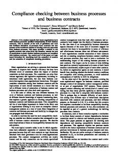
not contain deadlocks, and that each completion of a run is a proper termination, with no tokens remaining inside the process. These properties can be ensured using standard workflow validation techniques, e.g., [19,20]. For the annotations, we use standard notions from logics, involving logical predicates and constants (the latter correspond to the entities of interest at process execution time).4 We denote predicates with G, H, I and constants with c, d, e. Facts are predicates grounded with constants, Literals are possibly negated facts. If l is a literal, then ¬l denotes l’s opposite (¬p if l = p and p if l = ¬p); if L is a set of literals V then ¬L denotes {¬l | l ∈ L}. We identify sets L of literals with their conjunction l∈L l. Given a set P of predicates and a set C of constants, P[C] denotes the set of all literals based on P and C; if arbitrary constants are allowed, we write P[]. A clause is a universally quantified disjunction of atoms, e.g., ∀x.¬G(x) ∨ ¬H(x). A theory T is a conjunction of clauses.5 Our efficient algorithms will be designed for binary theories: a clause is binary if it contains at most two literals; a theory is binary if it is a conjunction of binary clauses. Note that binary clauses can be used to specify many common ontology properties such as subsumption relations ∀x.G(x) ⇒ H(x) (φ ⇒ ψ abbreviates ¬φ ∨ ψ), attribute image type restrictions ∀x, y.G(x, y) ⇒ H(y), and role symmetry ∀x, y.G(x, y) ⇒ G(y, x). An ontology O is a pair (P, T ) where P is a set of predicates (O’s formal terminology) and T is a theory over P (constraining the behaviour of the application domain encoded by O). Annotated process graphs are defined as follows. Definition 3. An annotated process graph is a tuple G = (N , E, O, A). (N , E) is a process graph, O = (P, T ) is an ontology, and A, the annotation, is a function mapping n ∈ NT ∪{n0 , n+ } to (pre(n), eff(n)) where pre(n), eff(n) ⊆ P[]. We require that there does not exist an n so that T ∧ eff(n) is unsatisfiable, or T ∧ pre(n) is unsatisfiable. We refer to cycles in (N , E) as loops. We refer to pre(n) as n’s precondition, and to eff(n) as n’s effect (sometimes called postcondition in the literature). The annotation of tasks – atomic actions that on the IT level can e.g., correspond to Web service executions – in terms of logical preconditions and effects closely follows Semantic Web service approaches such as OWL-S (e.g., [1,6]) and WSMO (e.g., [7]). All the involved sets of literals (pre(n), eff(n)) are interpreted as conjunctions. Similarly to Definition 1, the requirements stated in Definition 3 are just basic sanity checks. Example 1. Consider the annotated process graph depicted in Figure 2 (using the slightly extended BPNM notation from [4]). In short, data objects depict the entities of interest, and associations link them to activities. Preconditions and effects are displayed as text on the associations, where the preconditions are denoted subsequent to “” . In terms of the formal notations from Definition 3, this process graph is defined as follows (by the number of “.” symbols in the definition of logical predicates we indicate their arity): 4

5

Hence our constants correspond to BPEL “data variables” [15]; note that the term “variables” in our context is reserved for variables as used in logics, quantifying over constants. As indicated, our compliance rules are also clauses; however, their formal interpretation is different. This will be explained further below, when we formally introduce constraint bases.


51

Send PO

< PurchaseOrder (PO) > isSent(PO)

PO

Send cancellation

< PurchaseOrder (PO), isSent(PO) > isCancelled(PO)

Fig. 2. Basic example of a semantic process model (extended BPMN diagram). P := { PurchaseOrder(.), isCancelled(.), isSent(.)}; C := {P O}; T := ∅; NT := {n1 , n3 }; NXS := {n2 }; NXJ := {n4 }; E := {(n0 , n1 ), (n1 , n2 ), (n2 , n3 ), (n2 , n4 ), (n4 , n+ )}. The annotation function is given by the following: n1 (“Send PO”): pre(n1 ) := {PurchaseOrder(P O)} eff(n1 ) := {isSent(P O)} n3 (“Send cancellation”): pre(n3 ) := {PurchaseOrder(P O), isSent(P O)} eff(n3 ) := {isCancelled(P O)} This simplistic process sends out a purchase order, followed by an optional cancellation. This kind of process model combines a formalized view on both the process structure and the semantics of the individual activities. The semantics of individual activities is specified by capturing under which circumstances the execution of an activity in a process instance will change “the world” in which way – where “the world” is the relevant business domain as formalized by the underlying ontology. The formal execution semantics is defined as follows. Definition 4. Let G = (N , E, O, A) be an annotated process graph. Let C be the set of all constants appearing in any of the annotated pre(n), eff(n). A state s of G is a pair (ts , is ) where t is a token mapping and i is an interpretation i : P[C] 7→ {0, 1}. A start state s0 is (t0 , i0 ) where t0 is as in Definition 2, and i0 |= T [C] ∧ eff(n0 ). Let s and s0 be states. We say that there is a transition from s to s0 via n, written s →n s0 , iff one of the following holds: 1. n ∈ NP S ∪ NP J ∪ NXS ∪ NXJ , is = is0 , and ts →n ts0 according to Definition 2. 2. n ∈ NT ∪ {n+ }, ts →n ts0 according to Definition 2, is |= pre(n) and is0 ∈ min(is , T [C] ∧ eff(n)) where min(is , T [C] ∧ eff(n)) is defined to be the set of all i that satisfy T [C] ∧ eff(n) and that are minimal with respect to the partial order defined by i1 ≤ i2 :iff {p ∈ P[C] | i1 (p) = is (p)} ⊇ {p ∈ P[C] | i2 (p) = is (p)}. An execution path is a transition sequence starting in a start state s0 . A state s is reachable if there exists an execution path ending in s. Given an annotated process graph (N , E, O, A), we will use the term execution path of (N , E) to refer to an execution over tokens that acts as if no annotations were present.

52


The part of Definition 4 dealing with n ∈ NP S ∪ NP J ∪ NXS ∪ NXJ parallels Definition 2: the tokens pass as usual, and the interpretation remains unchanged. Consider now the start states, of which there may be many, namely all those that comply with T , as well as eff(n0 ) (if annotated). This models the fact that, at design time, we do not know the precise situation in which the process will be executed. All we know is that, certainly, this situation will comply with the domain behavior given in the ontology and with the properties guaranteed as per the annotation of the start node. The semantics of task node executions is the most intricate bit. First, for the obvious reasons, pre(n) is required to hold. The tricky bit lies in the definition of the possible outcome states i0 . Our semantics defines this to be the set of all i0 that comply with T and eff(n), and that differ minimally from i. Here we draw on the AI actions and change literature for a solution to the frame and ramification problems. The latter problem refers to the need to make additional inferences from eff(n), as implied by T ; this is reflected in the requirement that i0 complies with both. The frame problem refers to the need to not change the previous state arbitrarily – e.g., if an activity changes an account A, then any account B should not be affected; this is reflected in the requirement that i0 differs minimally from i. More precisely, i0 is allowed to change i only where necessary, such that there is no i00 that makes do with fewer changes. This semantics follows the possible models approach (PMA) [22]; while this approach is not entirely uncontroversial, it underlies all recent work on formal semantics for execution of Semantic Web services (e.g., [14,3,10]). Other semantics from the AI literature (see [13] for an excellent overview) could be used in principle; this is a topic for future research. In the rest of the paper, we assume that all task node are executable – whenever a task is activated, its preconditions are made true: for all reachable states s with ts (IN (n)) > 0, s |= pre(n); and that there are no effect conflicts: for any two parallel task nodes n1 and n2 , T ∧ eff(n1 ) ∧ eff(n2 ) is satisfiable. Both are desirable properties of any process; the properties can be validated using techniques currently under exploration by the authors, in other work; we assume that such a technique has completed successfully. 2.2

Constraint Bases

It remains to define what constraints and non-compliances are: Definition 5. Let G = (N , E, O, A) be an annotated process graph, where O = (P, T ). A constraints base B is a set of clauses. Let C be the set of all constants appearing in any of the annotated pre(n), eff(n), and let s be a reachable state. Then s is a non-compliance, or non-compliant state, iff there exists φ ∈ B such that s 6|= φ[C]. This definition is straightforward and should be self-explanatory. It should, however, be noted that the vocabulary for B and T is assumed to be the same here. I.e., with respect to using B to express compliance constraints, this means that the annotation of the process is assumed to refer to statements of interest to compliance checking. In practice, this may require additional modeling. The subtle point here is the distinction between B and T . Both are formalized similarly; the difference lies in how they are interpreted. T models the conditions that any


53

state must satisfy, due to the “physical” behavior of the underlying business domain (such as, any purchase order of a particular product is, in particular, a purchase order). In contrast, B models the conditions that any state should satisfy, in order to comply with the rules of the business (such as, for example, that the auditor for any activity is different from the actor who performed or authorised the activity – separation of duties). At a formal level, this difference is accounted for by using T as part of the definition how states evolve, while using B “only” to check whether the states are desirable or not.

3

Non-compliance Detection

We now specify two polynomial-time approximate methods to find non-compliances. Both methods rely on the information computed by a certain propagation algorithm, which is defined for a particular class of processes. We specify the propagation algorithm, then its use for compliance checking. 3.1

Propagation Algorithm

The algorithm finds, for every edge in the process, the set of literals that are always true when the edge is activated. The algorithm is defined for “basic” processes: Definition 6. Let G = (N , E, O, A), O = (P, T ), be an annotated process graph. G is basic if it contains no loops, and T is binary. It should be noted that the absence of loops is a strong requirement. We are currently working on extending our algorithms to be able to deal with loops. For complexity considerations, we assume fixed arity in the following, i.e., a fixed upper bound on the arity of predicates P. This is a realistic assumption because predicate arities are typically very small in practice (e.g., in Description Logics the maximum arity is 2). Given a process graph whose annotations mention the constants C, and a set L of literals (such as a task node effect), in the following we denote L := {l ∈ P[C] | T ∧ L |= l}, i.e., L is the closure of L under implications in the theory T . Since T is binary, L can be computed in polynomial time given fixed arity [2]. The algorithm performs three steps: (1) Determine a numbering # of the edges E so that, whenever task node n1 is ordered before task node n2 in every process execution, then #(IN (n1 )) < #(IN (n2 )). (2) Using #, determine all pairs of parallel task nodes. (3) Using that information, determine, for each edge e, the set of literals that is always true when e is active. In what follows, we explain in detail steps (2) and (3), in that order. Step (1) is relatively straightforward, and can be looked up in [21]. Step (2) propagates matrix functions M along the edges of the process graph. M contains one entry for every pair of edges in E; # is used for indexing into M . The propagation steps are defined below. We use the following helper notations: #−1 is the inverse function of #, i.e., #−1 (i) = e iff #(e) = i; given a node n, #INmax (n) := max{#(e) | e ∈ IN (n)} is the maximum number of any incoming edge, and similarly for #OU Tmin (n) and #OU Tmax (n).

54


Definition 7. Let G = (N , E, O, A) be an annotated process graph. A matrix M is a function M : {0, . . . , |E| − 1} × {0, . . . , |E| − 1} 7→ {0, 1, ⊥}. We define the matrix M0 as (M0 )ij = 0 if i = j, (M0 )ij = ⊥ otherwise. Let M and M 0 be matrices, n ∈ N . We say that M 0 is the propagation of M at n iff we have: j 6= ⊥. 1. For all j ∈ {0, . . . , #INmax }, we have M#(e) j = ⊥. 2. For all e ∈ OU T (n) and j ∈ {0, ..., |E| − 1} \ {#(e)}, we have M#(e)

As well as one of the following: 3. n ∈ NT and M 0 is given by M 0ij = Mji otherwise. 4. n ∈ NP S and  i M#(IN (n))     1 M 0ij =     i Mj 5. n ∈ NXS and  i M#(IN (n))     0 M 0ij =     i Mj

i M 0ij = M#(IN (n)) if #(OU T (n)) = j and i < j,

#−1 (j) ∈ OU T (n) and i < #OU Tmin (n) #−1 (j) ∈ OU T (n) and i 6= j and #OU Tmin (n) ≤ i ≤ #OU Tmax (n) otherwise. #−1 (j) ∈ OU T (n) and i < #OU Tmin (n) #−1 (j) ∈ OU T (n) and i 6= j and #OU Tmin (n) ≤ i ≤ #OU Tmax (n) otherwise.

6. n ∈ NP J and  i   1 #(OU T (n)) = j and i < j and for all e ∈ IN (n) : M#(e) = 1 i =0 M 0ij = 0 #(OU T (n)) = j and i < j and ex. e ∈ IN (n) : M#(e)   i Mj otherwise. 7. n ∈ NXJ , and for all e, e0 ∈ IN (n) we have M#(e) = M#(e0 ) , and M 0 is given i by M 0ij = M#(e) if #(OU T (n)) = j and i < j and e ∈ IN (n), M 0ij = Mji otherwise. If M ∗ results from starting in M0 , and stepping on to propagations until no more propagations exist, then we call M ∗ an M -propagation result. Definition 7 is hard to read; however, the underlying key ideas are simple. The matrix M annotated at edge e, at any point in time, provides complete information about all edges preceding e according to #; precedence according to # is meaningful because # respects task node orderings. The definition of M0 is obvious, likewise case 3 which handles task nodes. In a parallel split n (case 4), n’s OUT edges copy the information from n’s IN edge, except that the OUT edges are marked to be parallel with respect to each other. For xor splits (case 5), the OUT edges are marked to be not parallel with respect to each other. In a parallel join (case 6), an OUT edge is parallel to a preceding edge iff all IN edges are. Finally, xor joins (case 7) are only executed if all IN edges agree on parallelism: if they don’t, then the underlying workflow is unsound; if they do, then the OUT edge simply copies the information from the IN edges.


55

Lemma 1. Let G = (N , E, O, A) be an annotated process graph. There exists exactly one M -propagation result M ∗ , and for all n1 , n2 ∈ NT we have n1 k n2 iff #(IN (n )) M ∗ #(IN (n21 )) = 1. The time required to compute M ∗ is polynomial in the size of G. Proof Sketch: Uniqueness of M ∗ follows because 1 (2) requires all IN (OUT) edges to be determined (not determined), and any propagation affects only OUT edges. Parallelism between two nodes is determined by the routing constructs between the start node and these two nodes. Namely, we have n1 k n2 iff n1 and n2 have a common ancestor n ∈ NP S with no corresponding join node in between, and n1 and n2 do not lie on different sides of an xor-split. By construction of cases 4–7, which propagate #(IN (n )) exactly this information, these conditions hold true iff M ∗ #(IN (n21 )) = 1. Obviously, the propagation takes polynomial time. Having completed the computation of M ∗ , we can proceed to step (3) of the algorithm, determining, for each edge e, the set of literals that is always true when e is active. Again, this computation is based on propagation steps; this time, the propagations update sets of literals that are assigned to the edges. In the fixpoint, these literal sets are exactly the desired ones. The information from M ∗ is used to determine the “side effects” that any task node may have, on edges other than its own OUT edge. Definition 8. Let G = (N , E, O, A) be a basic annotated process graph without effect conflicts, and with constants C; let M ∗ be the M -propagation result. We define the function I0 : E 7→ 2P[C] ∪ {⊥} as I0 (e) = eff(n0 ) if e = OU T (n0 ), I0 (e) = ⊥ otherwise. Let I, I 0 : E 7→ 2P[C] ∪ {⊥}, n ∈ N . We say that I 0 is the propagation of I at n iff one of the following holds: 1. n ∈ NP S ∪NXS , and I(IN (n)) 6= ⊥, and for all e ∈ OU T (n) we have I(e) = ⊥, and I 0 is given by I 0 (e) = I(IN (n)) if e ∈ OU T (n), I 0 (e) = I(e) otherwise. 2. n ∈ NP J , and for all S e ∈ IN (n) we have I(e) 6= ⊥, and I(OU T (n)) = ⊥, and I 0 is given by I 0 (e) = e0 ∈IN (n) I(e0 ) if e = OU T (n), I 0 (e) = I(e) otherwise. 3. n ∈ NXJ , and for all T e ∈ IN (n) we have I(e) 6= ⊥, and I(OU T (n)) = ⊥, and I 0 is given by I 0 (e) = e0 ∈IN (n) I(e0 ) if e = OU T (n), I 0 (e) = I(e) otherwise. 4. n ∈ NT , and I(IN (n)) 6= ⊥, and I(OU T (n)) = ⊥, and    eff(n) ∪ (I(IN (n)) \ ¬eff(n)) e = OU T (n) #(e) I 0 (e) = I(e) \ ¬eff(n) M ∗ #(IN (n)) = 1 and I(e) 6= ⊥   I(e) otherwise If A(n) is not defined then eff(n) := ∅ in the above. If I ∗ results from starting in I0 , and stepping on to propagations until no more propagations exist, then we call I ∗ an I-propagation result. Like Definition 7, Definition 8 is a little hard to read but relies on straightforward key ideas. The definition of I0 is obvious. For split nodes (case 1), the OUT edges simply copy their sets from the IN edge. For parallel joins (case 2), the OUT edge assumes the union of I(e) for all IN edges e; for xor joins (case 3), the intersection is taken

56


instead. The handling of task nodes (case 4) is somewhat more subtle. First, although there are no effect conflicts it may happen that a parallel node has inherited (though not established itself, due to the postulated absence of effect conflicts) a literal which the task node effect contradicts; hence line 2 of case 4.6 Second, we must determine how the effect of n may affect any of the possible interpretations prior to executing n. This is non-trivial due to the complex semantics of task executions, based on the PMA [22] definition of minimal change for solving the frame problem, c.f. Section 2. Our key observation is: (*) With binary T , if executing a task makes literal l false in at least one possible interpretation, then ¬l is necessarily true in all possible interpretations. Due to this observation, it suffices to subtract ¬eff(n) in the top and middle lines of the definition of I 0 (e): l does not become false in any interpretation, unless ¬l follows logically from eff(n). Importantly, (*) does not hold for more general T ; see [21] for an example where T is Horn. Lemma 2. Let G = (N , E, O, A) be a basic annotated process graph where all n ∈ NT are executable and where there are no effect conflicts. There exists exactly one Ipropagation result I ∗ . For all e ∈ E, we have that l ∈ I ∗ (e) iff, for all reachable states s where ts (e) > 0, s |= l. With fixed arity, the time required to compute I ∗ is polynomial in the size of G. Proof Sketch: Uniqueness of I ∗ follows similarly as for Lemma 1. The second property is obvious for OU T (n0 ), as well as the outgoing edges of split nodes (case 1). If we join parallel branches, then all their results will be true (case 2). If we join alternative branches, then only their common results will be true (case 3). For task nodes (case 4), the above (*) shows that, with binary T , every literal l true at IN (n) remains true at OU T (n) unless its opposite ¬l can be derived from n’s effect. The time required to compute I ∗ is polynomial because, with fixed arity and binary T , the implications of a literal conjunction can be computed in polynomial time. 3.2

Compliance Checking

Once the propagation finished, we can use the outcomes to actually check the compliance of the process model. Based on the information provided by I ∗ , it is easy to devise two approximate methods for compliance checking. We need a few more notations. Say G = (N , E, O, A) is a basic annotated process graph with constants C. If I ∗ is the Ipropagation result, then for e ∈ E we denote U ∗ (e) := {l | l ∈ P[C], ¬l 6∈ I ∗ (e)}. If B is a constraints base, and φ = ∀X.ψ(X) is a clause in B, then any grounding ψ(C 0 ) of ψ with a tuple C 0 of constants from C is a grounded constraint. We identify ψ(C 0 ) with the set of literals it contains. It follows immediately from Lemma 2 that U ∗ (e) is exactly the set of literals that may be true when e is activated: l ∈ U ∗ (e) iff there exists a reachable state s such that ts (e) > 0 and s |= l. Further, it is obvious that any state s is a non-compliance iff it violates one of the grounded constraints. We hence get: 6

The interactions of parallel nodes with conflicting effects may be quite subtle, and require a much more complicated propagation algorithm.


57

Theorem 1. Let G = (N , E, O, A) be a basic annotated process graph where all n ∈ NT are executable and where there are no effect conflicts; let I ∗ be the I-propagation result. Then, for all e ∈ E: 1. If there exists a grounded constraint ψ(C 0 ) such that ¬ψ(C 0 ) ⊆ I ∗ (e), then every reachable state s with ts (e) > 0 is a non-compliance. 2. If there exists a non-compliant state s with ts (e) > 0, then there exists a grounded constraint ψ(C 0 ) such that ¬ψ(C 0 ) ⊆ U ∗ (e). Theorem 1 immediately suggests our two approximate methods: for every edge e, check whether there exists a grounded constraint ψ(C 0 ) such that 1. ¬ψ(C 0 ) ⊆ I ∗ (e), or 2. ¬ψ(C 0 ) ⊆ U ∗ (e). In the first case, we know for sure that a non-compliant state exists (presuming that a state activating e is reachable). In the second case, we know that a non-compliant state may exist; by contra-position, if the second test fails for all e then we know that the process complies with the constraints base. Clearly, if all predicates have a fixed arity and if the number of ground constraints is polynomial (i.e., if the number of variables in any constraint is fixed), then all the tests can be performed in polynomial time. Importantly, approximation is the best we can do with a polynomial-time algorithm: Theorem 2. Assume a basic annotated process graph G = (N , E, O, A) and a constraints base B. Deciding whether there exists a non-compliant state is NP-hard even if predicate arity is 0, T is empty, and B contains a single clause. Wn Proof. By a reduction from SAT. Say ψ = i=1 ψi is a propsitional CNF formula, over a set P of propositions. We take the set of predicates to be P ∪ {p1 , . . . pn } where p1 , . . . , pn are new. We take effn0 to be {¬p1 , . . . ¬pn }, so that the start states have all pi false and otherwise correspond to the set of interpretations of P . Our process is a sequence of n xor splits/joins, with several branches each. In the ith split/join, one “negative” branch consists of a task node with precondition {l | ¬l is contained in ψi } and no effect; there is one “positive” branch for every l contained in ψi , consisting of a task node with precondition l and effect {pi }. The single constraint is taken to be ¬p1 ∨ · · · ∨ ¬pn . The only chance to violate this constraint is to reach a state where a positive branch has been taken for every clause ψi . Obviously, this can be done if and only if ψ is satisfiable. Note that the hard bit in Theorem 2 lies in checking whether a set of literals can be true all at the same time. We have a single grounded constraint, ψ, and we have ¬ψ = {p1 , . . . , pn }. If e is, say, the outgoing edge of the nth xor join, then quite obviously we have I ∗ (e) = ∅ (unless one of the clauses is empty, or contains both a literal and its opposite, which cases we can exclude without loss of generality) and we have U ∗ (e) = {¬p1 , . . . ¬pn , p1 , . . . , pn }. So U ∗ (e) tells us that a non-compliance may exist – because each pi may be true – but it tells us nothing about whether we can actually make all the pi true at the same time.

4

Error Diagnosis

In order to efficiently support the user in compliance checking, it is of high value to be able to point out the sources of an error. Since we check the compliance rules against

58


summaries of the logical states that may occur, we can try to find out how the logical states leading to non-compliance came into being. When a particular state summary does not satisfy one of the compliance rules in the constraint base (and, thus, the related states are (potentially) non-compliant), then there is a set of literals which account for this behavior. We now need to trace back which activities in the process model caused these ground literals. This can be achieved by maintaining a support function for each ground literal, i.e., a (potentially empty or unary) list of process tasks whose effects lead to this ground literal, explicitly or implicitly. Formally, fs : L → {NT }; fs (l) := {n ∈ NT | l ∈ eff(n)}. It is easy to see that this support function can be created with little overhead during the I-propagation. Say, a constraint clause ψ does not hold for the I ∗ (e) or U ∗ (e) of some e. Then, we want to point out which tasks are responsible for this non-compliance. First, consider the case where ψ does not hold for I ∗ (e), formally: ¬ψ(C) ⊆ I ∗ (e). That means that we are guaranteed to have non-compliance, and we want to mark all tasks which contributed to this state. Any such task node n0 has the characteristics that it is executed before e, i.e., there is a path in the graph from n0 to n, with n being the node from which e originates: e ∈ OU T (n). Further, n0 contributes to the non-compliance, i.e., eff(n) ∩ ¬ψ(C) 6= ∅. Now consider the case where ψ does not hold for U ∗ (e), ¬ψ(C) ⊆ U ∗ (e), which means that non-compliance may occur. In this case there are two types of literals in ¬ψ(C): – Those literals which are contained in I ∗ (e), and hence will definitely occur. We refer to this set as A := ¬ψ(C 0 ) ∩ I ∗ (e). Their treatment is as in the first case, where we mark all actions which contribute to this circumstance. – Those literals which may occur, i.e., they are in U ∗ (e) but not in I ∗ (e). This set is called B := ¬ψ(C) \ I ∗ (e).7 For the literals in B it is rather interesting why it cannot be assumed that their involvement in the non-compliance has not been prevented. This may be the case because a task node n0 which is necessary for the prevention may not exist; or n0 may be only optional, and we can thus not assume it has been executed when e is activated; or n0 may be executed in parallel to n, where it should be executed before n; or n0 is positioned after n in the process. We thus mark all task nodes n0 with eff(n0 ) ∩ ¬(¬ψ(C) \ I ∗ (e)) 6= ∅, regardless of their position relative to n in the process graph. How the sets of nodes can be computed should be obvious, given the support function fs and the process graph. Once this is done, the marked tasks can be presented by the respective front-end in one way or another, e.g., by giving a list of non-compliance sources, or by graphically high-lighting the involved tasks.

5

Related Work

While the issue of compliance business process models with normative specification started receiving attention in the past few years, the study of how to formally represent 7

Note that A ∩ B = ∅ and A ∪ B = ¬ψ(C).


59

normative specifications has a long history and a full detailed comparison with the vast literature is out of the scope of the paper. In the context of this paper is worth remembering that the use of logical clauses for normative specifications goes back to Kowalski and Sergot [18], who proposed to encode regulations and normative systems as logic programs. More recently [8] proposed to use Event Calculus and logic programming as executable specifications for contracts, though the main focus is on monitoring the performance of a contract. [9] considers a similar approach where the tasks of a business process model, written in BPMN, are annotated with the effects of the tasks, and a technique to propagate and cumulate the effects from a task to a successive contiguous one is proposed. The technique is designed to take into account possible conflicts between the effects of tasks and to determine the degree of compliance a BPMN specification. Contrary to what we do this approach does not determine at design time whether a business process is both executable and compliant. [5] on the other hand investigates compliance in the context of agents and multi-agent systems based on a classification of paths of tasks. [16] proposed Concurrent Transaction Logic to model the states of a workflow and presented some algorithms to determine whether the workflow is compliant. The major limitation of most of the approaches to compliance is that they ignore the normative aspects of compliance. A notable exception is [12] that proposes to use FCL, a simple rule base logic enriched with deontic operators, to specify the obligations a process has to fulfil. They argue that compliance is the relationship between the potential execution states of a process and the normative specifications (resulting in the so called ideal-semantics). We plan to extend our work to incorporate FCL, for expressing the normative specifications and the current framework for the representation of the semantics of a business process for a more accurate analysis of the business process compliance phenomena.

6

Conclusion

We have presented a formalism for annotated process models, and we have devised approximate methods, with either a soundness or a completeness guarantee, for validating a process against a set of compliance rules in the form of disjunctive constraints that model which states are desirable. Of course, this is but a first step in exploring this form of compliance checking. First, there is a myriad of open questions within our current formalism: e.g., how to properly support loops? and how should we design compliance checking for computationally hard cases? Apart from this kind of issues, the formalism as such is lacking expressiveness in comparison to rich notions for compliance such as those in specialized formalisms as FCL. To cater for such compliance notions, beside the extension we discussed in the previous section, our formalism must be extended with, e.g., ways of expressing resource allocations and temporal aspects. While resource allocations may to some extent be expressible in terms of semantic annotations, temporal constructs add a whole new level of complexity to our framework; a possibly fruitful direction to handle the latter is to extend our propagation algorithm with time windows expressing when the literals will be necessarily true.

60


References 1. A. Ankolekar et al. DAML-S: Web service description for the semantic web. In ISWC, 2002. 2. B. Aspvall, M. Plass, and R. Tarjan. A linear-time algorithm for testing the truth of certain quantified boolean formulas. Information Processing Letters, 8:121–123, 1979. 3. F. Baader, C. Lutz, M. Milicic, U. Sattler, and F. Wolter. Integrating description logics and action formalisms: First results. In AAAI, 2005. 4. Matthias Born, Florian Dörr, and Ingo Weber. User-friendly Semantic Annotation in Business Process Modeling. In Hf-SDDM Workshop at WISE, 2007. 5. A. K. Chopra and M. P. Sing. Producing compliant interactions: Conformance, coverage and interoperability. In Declarative Agent Languages and Technologies IV, volume 4327 of LNAI, pages 1–15. Springer, 2007. 6. The OWL Services Coalition. OWL-S: Semantic Markup for Web Services, 2003. 7. D. Fensel et al. Enabling Semantic Web Services: The Web Service Modeling Ontology. Springer-Verlag, 2006. 8. A.D.H. Farrell, M.J. Sergot, M. Sallé, and C. Bartolini. Using the event calculus for tracking the normative state of contracts. International Journal of Cooperative Information Systems, 14(2-3):99–129, 2005. 9. A. Ghose and G. Koliadis. Auditing business process compliance. In Service Oriented Computing, ISOC 2007, LNCS, pages 169–180. Springer, 2007. 10. G. De Giacomo, M. Lenzerini, A. Poggi, and R. Rosati. On the update of description logic ontologies at the instance level. In AAAI, 2006. 11. G. Governatori and Z. Milosevic. A formal analysis of a business contract language. International Journal of Cooperative Information Systems, 15(4):659–685, 2006. 12. G. Governatori, Z. Milosevic, and S. Sadiq. Compliance checking between business processes and business contracts. In Patrick C. K. Hung, editor, 10th International Enterprise Distributed Object Computing Conference (EDOC 2006), pages 221–232. IEEE Computing Society, 16–20 October 2006. 13. A. Herzig and O. Rifi. Propositional belief base update and minimal change. Artificial Intelligence, 115(1):107–138, 1999. 14. C. Lutz and U. Sattler. A proposal for describing services with DLs. In DL, 2002. 15. OASIS. Web Services Business Process Execution Language Version 2.0, April 2007. 16. D. Roman and M. Kifer. Reasoning about the behaviour of semantic web services with concurrent transaction logic. In VLDB, pages 627–638, 2007. 17. S. Sadiq, G. Governatori, and K. Namiri. Modelling control objectives for business process compliance. In Proc. 5th International Conference on Business Process Management, Brisbane, Australia, 24-28 September 2007. 18. M. J. Sergot, F. Sadri, R. A. Kowalski, F. Kriwaczek, P. Hammond, and H.T. Cory. The british nationality act as a logic program. Commun. ACM, 29(5):370–386, 1986. 19. W. van der Aalst and K. van Hee. Workflow Management: Models, Methods, and Systems. The MIT Press, 2002. 20. J. Vanhatalo, H. Völzer, and F. Leymann. Faster and more focused control-flow analysis for business process models though sese decomposition. In ICSOC, 2007. 21. I. Weber, G. Governatori, and J. Hoffmann. Approximate compliance checking for annotated process models. Technical report, School of ITEE, University of Queensland, 2008. Available at http://espace.library.uq.edu.au/eserv/UQ:135106/ tr-grcis08.pdf. 22. M. Winslett. Reasoning about actions using a possible models approach. In AAAI, 1988. 23. M. zur Muehlen, M. Indulska, and G. Kemp. Business process and business rule modeling languages for compliance management: A representational analysis. In Intl. Conf. Conceptual Modelling (ER) - Tutorials, Posters, Panels and Industrial Contributions, 2007.