Jul 31, 2017 - Wishart distribution, which is a very well-studied matrix distribution [1]. ... matrix distributions by central Wishart by means of Taylor expansion is ...
1
Approximate Random Matrix Models for Generalized Fading MIMO Channels Muralikrishnan Srinivasan
Sheetal Kalyani
arXiv:1707.09734v1 [cs.IT] 31 Jul 2017
Department of Electrical Engineering, Indian Institute of Technology, Madras, Chennai, India 600036.
{ee14d206,skalyani}@ee.iitm.ac.in
Abstract Approximate random matrix models for κ − µ and η − µ faded multiple input multiple output (MIMO) communication channels are derived in terms of a complex Wishart matrix by keeping the degree of freedom constrained to the number of transmitting antennas and by matching matrix variate moments. The utility of the result is demonstrated in a) computing the average capacity/rate of κ−µ/η−µ MIMO systems b) computing Symbol Error Rate (SER) for optimum combining with Rayleigh faded users and an arbitrary number of κ − µ and η − µ faded interferers. These approximate expressions are compared with Monte-Carlo simulations and a close match is observed.
Index Terms Random matrices, Wishart matrices, Generalized fading, κ − µ, η − µ, MIMO, capacity, optimum combining
I. I NTRODUCTION The need for high data rates has been one of the driving factors for the evolution of the wireless systems from Single Input Single Output (SISO) systems to Multiple Input Multiple Output (MIMO) systems. MIMO systems are being used increasingly in modern wireless standards and it is imperative to study the channel capacity and other Quality of Service (QoS) metrics of such systems. The capacity of wireless channels depends on channel fading statistics and also on whether the statistics are known at the receiver and the transmitter. To capture the fading statistics, channel
August 1, 2017
DRAFT
2
gain is characterized by a single random variable in SISO systems. But for MIMO systems, the channel is in the form of a matrix, hence the characterization of random matrices plays an indispensable role in studying MIMO channel metrics. The MIMO system is mathematically modeled by an NR × NT channel gain matrix H, where NR is the number of receive antennas and NT is the number of transmit antennas. Various performance metrics such as capacity, rate, etc. require the eigenvalue statistics of the Gram matrix HHH (or HH H). When the elements of H are i.i.d. circular symmetric complex Gaussian with zero or non-zero mean, i.e., when Rayleigh or Rician faded MIMO channels are considered, the Gram HHH can be characterized by Wishart matrices - central or non-central respectively [1]. These random matrix models have been used widely for deriving capacity expressions in the case of Rayleigh faded MIMO channels [2]–[4] and also Rician faded MIMO channels [5], [6]. Recently, there has been significant focus on generalized fading models namely κ − µ and η −µ models introduced in [7]. These distributions model the small scale variations in the fading channel in the line of sight and non-line of sight conditions respectively. Further, these generalized fading distributions include Rayleigh, Rician, Nakagami, One-sided Gaussian distributions as special cases. These generalized fading distributions have been widely used in capacity and outage probability analysis for SISO and MISO systems. Average channel capacity of single branch κ − µ and η − µ faded receivers is studied in [8]. The outage, coverage probability and rate of these generalized fading channels are analyzed in [9]–[13] and references therein. Secrecy capacity analysis is carried out in [14] and effective throughput in MISO systems is determined in [15], [16]. Outage probability of MRC in κ − µ fading channels in the presence of co-channel interference is studied in [17]. Analysis of decode and forward relay system for generalized fading models is performed in [18]–[20]. The capacity of MIMO systems for these generalized fading channels has been less analyzed for want of a random matrix model that characterizes the channel matrix. Nevertheless, some random matrix models have been developed for Nakagami and Rician-shadowed fading channels. A random matrix model has been developed for Nakagami-q fading in [21] and the pdf of eigen values of the Gram HHH is obtained in terms of a Pfaffian. In [22], the ergodic capacity of MIMO correlated Nakagami-m fading channel has been derived using the concept of a copula. But the work presents an analysis only for 2 × 2 MIMO channel and determining the capacity of MIMO channels with a larger number of receive and transmit antennas using this method is cumbersome. Recently a MIMO capacity upper bound was derived for the κ − µ and η − µ August 1, 2017
DRAFT
3
fading channels in [23]. In [24], a MIMO model has been developed for Rician-shadowed fading as a unification model for MIMO-Rayleigh and MIMO-Rician fading models. Given the complicated pdf structure of complex κ − µ and η − µ fading distributions [25],
[26], it is challenging to develop the matrix distribution and the eigenvalue statistics for HHH , even when the elements of H are assumed to be i.i.d. κ − µ or η − µ random variables. Hence,
in this paper, we develop an approximate matrix model for HHH (or HH H) in terms of a Wishart distribution, which is a very well-studied matrix distribution [1]. Approximating any matrix distributions by central Wishart by means of Taylor expansion is studied in [27], but the approximation requires the knowledge of not only one or more cumulants and moments of the random matrix that is to be approximated but also the derivatives of central Wishart matrix. Also, the approximation of non-central Wishart matrix by a central Wishart by means of Laguerre polynomial expansion is given in [28] and by means of the moment generating functions in [29]. In this paper, we propose a Wishart distributed approximation of HHH , such that the approximation has its first moment matched with the original matrix distribution of HHH and the degree of freedom is constrained to be the number of columns of the matrix H. This method requires only the knowledge of the expectation of HHH with respect to the original distribution and this can be found out for both the κ − µ and η − µ case. We also show that our method is equivalent to minimizing the K-L divergence between the actual MIMO matrix and the Wishart distributed approximation1. The proposed approximation is discussed in Section II. In Section III, the utility of the approximation is shown in two applications. In one application, the proposed approximation is used to determine the capacity of MIMO systems with i.i.d. κ − µ or η − µ channel gains. Further, the approximation is also used to determine the asymptotic capacity of these MIMO systems. To the best of our knowledge, ours is the first work to derive even an approximate capacity expression in the presence of κ − µ/η − µ MIMO channels. Another application of the approximation is in determining the Symbol Error Rate (SER) of an optimum combining (OC) receiver [30] for Rayleigh faded user and κ−µ or η−µ faded interferers. The SINR expression for OC involves a covariance matrix formed by interferer channel gains. Using the derived Wishart approximation, closed form expressions for SER of OC systems for κ − µ or η − µ faded 1
Since the κ − µ/η − µ fading distributions are fairly complicated, computing and matching the higher moments is fairly
difficult.
August 1, 2017
DRAFT
4
interferers are obtained. To the best of our knowledge, no prior work has given SER expressions for a receiver diversity system employing OC under the case of Rayleigh faded user and κ−µ or η−µ faded interferers. In Section IV, the derived capacity and SER approximations are compared with Monte-Carlo simulations and a close match is found between the theoretical results and simulation results. While we have only shown the utility of the approximation in two applications namely capacity computation and SER computation in OC system, the approximation can be used in any application which deals with random κ − µ/η − µ matrix models. Basic notation: Ex (.) denotes expectation with respect to distribution x. |X| and det(X) denote determinant of a matrix X. etr(X) denotes an exponential raised to trace of the matrix X. II. P ROPOSED A PPROXIMATION Let H be an n1 × n2 random matrix with independent and identically distributed elements.
and X = HHH be an n1 × n1 random matrix. The exact matrix distribution of X denoted by
p(X) is not known2. Hence, we propose to approximate the density p(X) by an n1 × n1 Wishart matrix whose distribution is q(X) = CW n1 (n2 , Σ) with n2 degrees of freedom and covariance matrix Σ, such that Ep [X] = Eq [X], i.e., their first moments are matched. Eq (X) = n2 Σ = Ep [X].
(1)
We now show that this is also equivalent to minimizing the the K-L divergence between p(X) and a Wishart distribution. Let q(X) be that Wishart distribution which minimizes the K-L divergence between p(X) and all the Complex Wishart distributions CW n1 (n, Σ), i.e., Z q(X) = argminKL(p(X)||q(X)) = argmax p(X)[ln(q(X)) − ln(p(X))]dX q(X)
q(X)
= argmax q(X)
Z
p(X)ln(q(X))dX.
(2)
Note that we assume an unknown degrees of freedom as n in this case, while in the Wishart approximation we had constrained the degree of freedom to n2 . The density of an n1 × n1 complex Wishart matrix X ∼ CW n1 (n, Σ) is given by [31], q(X) =
2
1 etr(−Σ−1 X)(detX)n−n1 , CΓn1 (n)(detΣ)n
The pdf of entries of H are known. But finding the matrix variate pdf of X = HHH is fairly complicated, since we require
the joint pdf of all entries of X. On the other hand, the diagonal elements of X are well characterized.
August 1, 2017
DRAFT
5
where CΓ. (.) is the complex multivariate gamma function [31]. Substituting the density in (2), we obtain q(X) = argmax q(X)
Z
�
� p(X) − ln(CΓn1 (n)) − nln|Σ| + T r(−Σ X) + (n − n1 )ln|X| dX −1
� � −1 = argmax − ln(CΓn1 (n)) − nln|Σ| + T r(−Σ Ep [X]) + (n − n1 )Ep [ln|X|] . q(X)
Denoting Z = Ep [X] and Y = Ep [ln|X|], we get � � −1 q(X) = argmax − ln(CΓn1 (n)) − nln|Σ| + T r(−Σ Z) + (n − n1 )Y .
(3)
q(X)
To obtain the minimizing distribution, we can differentiate the above equation with respect to two variables namely, Σ and n. Differentiating equation (3) w.r.t. Σ, we obtain dq(X) = −nΣ−1 + Σ−1 ZT Σ−1 . dΣ When the above equation is equated to zero, we obtain Σ=
1 1 T Z = Ep [X]. n n
(4)
Note that we obtain the same Σ when we equate the expectations of the matrix with respect to distributions p(X) and q(X), i.e., Ep [X] = Eq [X] and by fixing the degrees of freedom to be n2 . But the question arises as to whether the degree of freedom of the distribution obtained from minimizing K-L divergence is indeed n2 , which is nothing but the number of columns of the matrix H. In order to answer this question, we will continue the K-L divergence minimization by differentiating (3) w.r.t. n. Now differentiating equation (3) w.r.t. n, we obtain n
1 X dq(X) = −ln|Σ| + Y − ψ(n − i + 1), dn i=1
where ψ(.) is the digamma function [32]. Equating the derivative to zero, we get −ln|Σ| + Y − By substituting Σ =
1 T Z n
n1 X i=1
ψ(n − i + 1) = 0.
from (4), we obtain, ln(n) − ln|Z| + Y −
n1 X i=1
ψ(n − i + 1) = 0.
(5)
Matching the expectations Ep [ln|X|] = Eq [ln|X|] also leads to (5). Hence minimizing the K-L divergence has reduced to a simple case of matching expectations Ep [X] and Ep [ln|X|] with Eq [X] and Eq [ln|X|] respectively. August 1, 2017
DRAFT
6
Solving (5) for n requires the knowledge of Y = Ep [ln|X|]. Since finding the random matrix variate distribution of X is mathematically intractable, finding the expectation of the log-determinant analytically is not possible. We now argue that approximating n by n2 is a plausible solution to the problem. a) While Y = Ep [ln|X|] cannot be theoretically computed, it can be empirically computed by using simulated κ − µ/η − µ matrix elements and then solving for n in (5). We observe that in all our simulations, this leads to n being a real number which is very close to n2 . b) Note, n2 denotes the number of transmitter antennas or the number of interferers in the MIMO channel matrix. Hence, it makes sense to retain the same number n2 , even in approximation, given that there is no correlation in the transmitter side and all the elements of the matrix are i.i.d. c) For any Wishart distributed matrix A = BBH ∼ CW n1 (n2 , Σ), the degrees of freedom also denote the number of columns of complex Gaussian B. In fact, when a non-central Wishart matrix was approximated by a Wishart matrix in [29], the approach of keeping n = n2 was followed. Based on the above reasoning it can be argued that, n ≈ n2 . Hence, the minimizer complex
Wishart distribution, q(X) given by CW n1 (n2 , n12 ZT ), where Z = Ep [X], is the closest to the
actual unknown distribution among all central Wishart distributions in terms of K-L divergence. We will now apply the approximation procedure to i.i.d. κ − µ and η − µ fading MIMO channels and theoretically determine the covariance matrix Σ =
1 (Ep [X])T n2
=
1 T Z n2
of the corresponding
approximate Wishart matrix. Once the first moment is matched by the above procedure, we now quantify how close the second moment of the two matrices are to one another. For this, we determine NMSE (Normalized � � ˆ = P XXH − Mean Square Error) between the second moments of the two matrices. First, let X P� � P � ′ ′H � . denotes the empirical X X , where X′ is the Wishart approximated matrix and
average of a matrix. Also, X = HHH where H is a matrix with i.i.d. κ − µ elements. In ˆ is used to measure the discrepancy between the second moments of the actual other words, X
matrix and Wishart distributed approximation. Second, we determine the absolute value of all ˆ i.e., X(i, ˆ j)|. We now determine NMSE, i.e., the ratio ˜ j) = |X(i, the elements of the matrix X, � P� ˜ to the average of elements of XXH as of average of elements of X NMSE =
August 1, 2017
˜ T 1X1 � . P� XXH 1T 1
DRAFT
7
TABLE I: NMSE for n1 = 2 n2
κ = 2 and µ = 3
κ = 6 and µ = 3
κ = 2 and µ = 6
κ = 6 and µ = 6
2
0.4247
0.4633
0.4631
0.4769
4
0.2182
0.2328
0.2362
0.2417
6
0.1511
0.1563
0.1574
0.1631
8
0.1115
0.1198
0.1195
0.1205
Table I shows the NMSE for various values of degree of freedom n2 , κ and µ. We can see that as the degree of freedom n2 increases, NMSE decreases, i.e., the approximation becomes tighter, where as, if κ or µ increases, NMSE increases. A. κ − µ model In κ − µ fading model, the signal is divided into different clusters of waves. The number of clusters is µ and in each of the clusters, there is a deterministic LOS component with arbitrary power and scattered waves with identical powers. Note, κ is the ratio between the total power of the dominant components and the total power of the scattered waves. Suppose the elements hi,j = xij + jyij of H are i.i.d. κ − µ random variables, where xij and yij are the real and imaginary components respectively, then the joint distribution is given by [25], (xij − p)2 + (yij − q)2 |xij yij |µ/2 exp(− ) fxy (xij , yij ) = 4 4σ |pq|µ/2−1 2σ 2 qyij |pxij | |qyij | pxij (6) sech( 2 )sech( 2 )I µ2 −1 ( 2 )I µ2 −1 ( 2 ). σ σ σ σ P P Here p2 = µi=1 p2i and q 2 = µi=1 qi2 , where pi and qi are the LOS components of in-phase and
quadrature components respectively of multipath waves of each cluster. κ =
p2 +q 2 , 2µσ2
where σ 2 is
the power of the scattered waves. We are interested in the distribution of HHH . However, an exact characterization of the matrix variate distribution is intractable, because it involves finding the joint pdf of entries of HHH . Hence, we now approximate HHH by the Wishart matrix with n2 degrees of freedom and Σ =
1 E [HHH], n2 p
where the expectation is with respect to the κ − µ
pdf. The diagonal elements of Z = Ep [HHH ], i.e, zii are nothing but the mean of n2 κ − µ
August 1, 2017
DRAFT
8
envelope square variables. i.e., zii = E[ where κ =
p2 +q 2 . 2µσ2
zij = E[
n2 X k=1
P n2
2 j=1 [xij
+ yij2 ]]. Hence, zii = 2σ 2 n2 (1 + κ)µ from [7],
The off diagonal elements of zij are given by [(xik + jyik )(xkj − jykj )]] =
Since xik and yik are i.i.d., we obtain ∀i, j, zij =
n2 X
n2 X k=1
E[xik xkj + yik ykj − jxik ykj + jxkj yik ].
((E[xik ])2 + (E[ykj ])2 ).
(7)
k=1
E[xik ] and E[yik ] are given by, Z ∞ (x − p)2 px |x|µ/2 |px| E[xik ] = )sech( 2 )I µ2 −1 ( 2 )dx x 2 µ/2−1 exp(− 2 2σ σ σ −∞ 2σ |p| ∞
(y − q)2 qy |y|µ/2 |qy| µ )sech( )I )dy. E[yik ] = y 2 µ/2−1 exp(− ( −1 2σ 2 σ2 2 σ2 −∞ 2σ |q| Z
(8)
(9)
∀i, j. The closed form expressions for the above integrals seem mathematically intractable. However an approximation for the integral is derived in Appendix A and given by (39) and (40).
3
Since all the κ − µ elements of the matrix H are i.i.d., the mean of all the off-diagonal
elements are equal. Substituting the results from (39) and (40) in (7), we obtain ∀i, j and i 6= j, " µ i2 h p2 µ µ 2p2 π 2p2 4σ 2 µ +1 Γ( 2 + 1) 2 ) + 1, 1, 3/2, , , ) zij ≈ n2 2pe− 2σ2 ( 2 Ψ ( 1 4σ + 2p2 π Γ( µ2 ) 2 2 2p2 π + 4σ 2 4σ 2 + 2p2 π # µ h i2 2 2 2 q2 + 1) Γ( µ µ µ 2q π 2q 4σ + 2qe− 2σ2 ( 2 ) 2 +1 2 µ Ψ1 ( + 1, 1, 3/2, , 2 , ) . 2 4σ + 2q π Γ( 2 ) 2 2 2q π + 4σ 2 4σ 2 + 2q 2 π
(10)
Since Σ =
Z , n2
we have Σii = 2σ 2 (1 + κ)µ and Σij = zij /n2 , i 6= j
(11)
Now we look at a special case of κ − µ distribution namely the Rician distribution with µ = 1. 3
These closed form approximations are also compared with both numerical integration evaluation of (8) and (9) and Monte-
Carlo simulation and an excellent match is observed with both.
August 1, 2017
DRAFT
9
Rician: Suppose the elements hi,j = xij + jyij ∼ CN (pij + jqij , 2σ 2 ) of H are independent Rician distributed random variables, where xij and yij are the real and imaginary components respectively, then the joint distribution is given by [25], fxy (xij , yij ) =
(xij − pij )2 + (yij − qij )2 1 exp(− ) 2πσ 2 2σ 2
2 p2ij +qij . 2 2σ
The diagonal elements zii of n2 Σ are nothing but mean P 2 2 of n2 sum of Rician envelope square variables. i.e., zii = E[ nj=1 [xij + yij2 ]] = 2σ 2 n2 (1 + κ) P 2 (pik + jqik )(pkj − jqkj ). and the off-diagonal elements zij = nk=1
with identical Rice factor κ =
Since the elements of H have a Rician envelope, X is a non-central Wishart matrix. In
this case, we are simply approximating a non-central Wishart matrix by a central Wishart matrix. This has been well studied in [29], which obtains the same approximation as us, but by deriving the moment generating function (mgf) of the non-central Wishart matrix and retaining the same degree of freedom. If the columns of the matrix H with dimension n1 × n2 are
distributed as complex Gaussian CN (mi , Σ′ ), then X is a non-central Wishart matrix distributed as CW n1 (n2 , Σ′ , MMH ), where M = [m1 , m2 , ..., ms ]. From [29], a non-central Wishart
matrix CW n1 (n2 , Σ′ , MMH ) can be approximated by a Wishart matrix CW n1 (n2 , Σ), where Σ = Σ′ +
1 MMH . n2
It is also known that the approximation becomes tighter as the degree of
freedom n2 increases. In our case also, it can be shown that Σ = Σ′ +
1 MMH . n2
If the variables are identically distributed, i.e., pij s are equal to p and qij s are equal to q, then the off-diagonal elements are n2 (p2 + q 2 ) = 2σ 2 n2 κ and it can be seen from a numerical evaluation that it is approximately equal to (10) evaluated at µ = 1. B. η − µ model The η − µ is a fading distribution that represents small scale fading effects in non-line of sight condition. The elements hij of H are independent and identical η − µ distributed random variables with density [26], � x2 yij2 � µ2µ |xij yij |2µ−1 ij + ) exp(−µ fxy (xij , yij ) = ΩµX ΩµY Γ2 (µ) ΩX ΩY
(12)
where Ω is the power parameter given by Ω = 2σ 2 µ, σ 2 is the power of the Gaussian variable in each cluster, µ is the number of clusters. Note, ΩX = (1 − η)Ω/2, ΩY = (1 + η)Ω/2, −1 ≤ η ≤ 1 and the diagonal elements zii are means of sums of η − µ envelope square
August 1, 2017
DRAFT
10
variables. i.e., zii = E[ elements are given by,
P n2
2 j=1 [xij
+ yij2 ]]. Hence by [7], zii = n2 (ΩX + ΩY ). The off-diagonal
n2 X zij = E[ [(xik + jyik )(xkj − jykj )]] k=1
Since xik and yik are i.i.d., we obtain ∀i, j and i 6= j, n2 X (E[xik ]2 + E[ykj ]2 ) = 0 zij = k=1
The off-diagonal elements are zero, because distributions fx (xij ) and fy (yij ) are odd functions. Therefore, Σ = (ΩX + ΩY )In1 . It is interesting to note that, the approximation doesn’t depend on η. C. Nakagami-m model The elements hij of H are independent and identically distributed Nakagami-m variables with density, fxy (xij , yij ) =
m mm |xij |m−1 |yij |m−1 exp(− (x2ij + yij2 )) m 2 Ω Γ (m/2) Ω
We can obtain a Nakagami random variable by substituting η = 0 i.e., ΩX = ΩY = Ω/2 and m = 2µ in η − µ random variable given by (12). It can also be obtained by substituting κ = 0
i.e., p = q = 0 and Ω = 2µσ 2 in κ−µ random variable given by (6). Hence, both the approaches
yield the same result, i.e., Σ = ΩIn1 . It is interesting to note that, existing work [22] has analyzed MIMO ergodic capacity of correlated Nakagami-m fading channels and derived a joint pdf of eigen-values of HHH using copula. But the analysis is performed only for 2 × 2 channel matrix and it becomes fairly difficult even for a 3 × 3 channel matrix. III. A PPLICATIONS
OF THE APPROXIMATION
In this section, to demonstrate the utility of our work, we apply the above approximation in two very different applications namely, finding MIMO channel capacity for κ − µ/η − µ faded channel coefficients and finding SER expressions for optimum combining with κ − µ/η − µ faded interferers. Finding ergodic MIMO channel capacity involves finding the expectation of log determinant of Gram matrix HHH , where entries of H are κ − µ/η − µ faded. On the other hand, finding SER expressions for optimum combining involves determining the SINR given by η = cH R−1 c, where R = HHH is the Gram matrix formed by κ − µ/η − µ faded interferers and c is the user signal.
August 1, 2017
DRAFT
11
A. MIMO channel Capacity We consider an NR × NT MIMO channel matrix H, where NR denotes the number of receive antennas and NT denotes the number of transmit antennas. Let x be the NT × 1 transmitted vector and n be the NR ×1 zero mean i.i.d. complex Gaussian noise vector. The NR ×1 received vector y is given by, y = Hx+n. Assuming that the transmitter has no channel state information (CSI), the capacity of the MIMO channels when the transmitter has no CSI, is given by [3], C ′ = log2 det(I +
ρ HHH ), NT
(13)
where ρ is the average signal to noise ratio (SNR) per receiving antenna. Since HHH and HH H have the same non-zero eigenvalue statistics, from [3], ′
C =
n1 X i=1
log2 (1 +
ρ λi ), NT
where n1 = min(NR , NT ) and λ1 , ...., λn1 are the non-zero eigenvalues of R, which is given by, HHH if NR ≤ NT R= HH H if NR > NT .
Hence, the mean value of C ′ is given by [2], n1 hX i ρ C = EΛ log2 (1 + λi ) . NT i=1
We do not know the exact eigenvalue distribution of R, when H comprises i.i.d. κ − µ or η − µ variables. Hence, we apply the Wishart approximation developed in the last section and then determine C. We approximate R by a Wishart matrix with a degree of freedom NT and NR ×NR covariance matrix Σ, given by (11) for κ − µ interferers and (ΩX + ΩY )INR for η − µ interferers. 1) κ − µ: The approximate expression for C is derived in Appendix. B. For NT ≥ NR , by substituting n2 = NT and n1 = NR in (44), we can get the average capacity approximation as, C ≈ (−1)
1 N (NR −1) 2 R
1 QNR
1
NT (w − w )NR −1 2 1 j=1 (NT − j)! (detΣ)
QNR −2 j=1
j!
NX R −1 k=1
|N k |,
(14)
where N k is given in (45) and w1 = 2σ 2 (1 + κ)µ − y and w2 = 2σ 2 (1 + κ)µ + (NR − 1)y are
the eigenvalues of Σ−1 with multiplicity NR − 1 and 1 respectively.
In case NT < NR , we approximate HH H instead of HHH since both have the same non-zero
eigenvalues. We therefore approximate HH H by a central Wishart W ∼ CW NI (NR , Σ). For
August 1, 2017
DRAFT
12
NT ≤ NR , by substituting n2 = NR and n1 = NT in (44), we can get the capacity approximation as, 1
C ≈ (−1) 2 NT (NT −1) QNT
1
1
j=1 (NR − j)!
k
|Σ|NR (w
2
− w1
)NT −1
2
QNT −2 j=1
2
j!
NX T −1 k=1
|N k |,
(15)
where N is given in (45) and w1 = 2σ (1 + κ)µ − y and w2 = 2σ (1 + κ)µ + (NT − 1)y are the eigenvalues of Σ with multiplicity NT − 1 and 1 respectively.
2) η−µ: If R = HHH with H having i.i.d. η−µ elements, we use the Wishart approximation
of R and follow a procedure similar to that used for κ−µ. For NT ≥ NR , by substituting n2 = NT and n1 = NR in (46), we can obtain the capacity approximation as, N
R X ((ΩX + ΩY ))−NR NT |N k |, C ≈ QNR QNR i=1 (NR − i)! k=1 i=1 (NT − i)!
(16)
where N k is given by (47). Similarly for NT ≤ NR , by substituting n2 = NR and n1 = NT in (46), we can obtain the capacity approximation as, N
T X ((ΩX + ΩY ))−NR NT |N k |, C ≈ QNT QNT i=1 (NT − i)! k=1 i=1 (NR − i)!
(17)
where N k is given by (47). Since, ΩX = (1 − η)Ω/2 and ΩY = (1 + η)Ω/2, the approximate capacity expressions depends only on the power parameter Ω and not on the η parameter. In [5] and [2], exact capacity expressions are derived for Rayleigh faded MIMO channels. The results from these expressions match our η/µ capacity expressions for Rayleigh faded MIMO channels, i.e., for η = 0 and µ = 1. Also, an upper bound for the ergodic capacity of κ − µ and η − µ faded MIMO channels is derived in [23]. However, the upper bound requires computation of the mean of each entry of H given by E[hij ], for which a numerical computation is done in [23]. Hence, we can apply our mean approximation in [23] to evaluate the upper bound. The upper bound is plotted in Section IV and compared with our theoretical approximation. 3) Asymptotics: Since we have approximated η − µ faded MIMO channels by a complex Wishart matrix, a lot of existing properties and results of complex Wishart matrix can be exploited to get interesting results for these channels. One such application is in determining the asymptotic capacity of generalized fading channels, especially η −µ faded channel. The asymptotic capacity of Rayleigh faded channels is studied in detail in [33]. We now use their analysis to study η − µ asymptotics. For NT = NR = N, and η − µ fading, the capacity is given by C = EΛ
N X i=1
August 1, 2017
log2 (1 +
ρ(ΩX + ΩY ) λi ), N
DRAFT
13
where λi are the eigen values of H ∼ CN N (0, IN ). Using [33], we obtain the asymptotic capacity as
where
Z ∞ N ρ(ΩX + ΩY ) 1 X log2 (1 + λi ) = log2 (1 + ρ(ΩX + ΩY )λ)g(λ)dλ lim EΛ N →∞ N i=1 N 0 g(λ) =
q 1 1 − π λ 0
1 4
0≤λ≤4
(18)
(19)
o.w.
Solving the above integral, we obtain the asymptotic capacity as N ρ ρ(ΩX + ΩY ) 3 F2 (1, 1, 3/2; 2, 3; −4ρ(ΩX + ΩY )) 1 X log2 (1 + λi ) = . lim EΛ N →∞ N i=1 N ln2
(20)
where 3 F2 (.) is a Hypergeometric function. With a first order approximation of the logarithm at low SNR as in [33], 1 lim C≈ N →∞ N
Z
∞
ρ(ΩX + ΩY )λg(λ)dλ = ρ(ΩX + ΩY ).
0
Similarly at high SNR, we obtain from [33], 1 C ≈ log2 (ρ(ΩX + ΩY )/e). N →∞ N lim
Since (ΩX + ΩY ) = Ω = 2µσ 2 , the capacity grows as a linear function of µ and SNR ρ, at low SNR and capacity grows as a logarithmic function of µ and SNR ρ, at high SNR. For κ − µ random variables, the capacity is given by C = E[log2 det(I +
ρ HHH )], N
(21)
where H ∼ CN N (0, Σ) and w1 = 2σ 2 (1 + κ)µ − y and w2 = 2σ 2 (1 + κ)µ + (N − 1)y are the eigenvalues of Σ with multiplicity N − 1 and 1. Unlike η − µ random variable, it is difficult to obtain the asymptotic capacity like in (20) for all SNR values, due to the presence of correlation matrix Σ. Hence, we will derive approximate asymptotic capacity only at high SNR. At high SNR, the capacity is given by ρ ρ HHH )] = E[log2 det( Σ1/2 H′ H′H Σ1/2 )] N N ρ ′ ′H = E[log2 det( H H )] + log2 det(Σ) N N X ρ = EΛ log2 ( λi ) + log2 (w1N −1 w2 ). N i=1
C ≈ E[log2 det(
August 1, 2017
DRAFT
14
where H′ ∼ CN N (0, I). Therefore, the asymptotic capacity is given by, N
N −1 1 ρ 1 X 1 log2 ( λi ) + lim C ≈ lim EΛ log2 (w1 ) + lim log2 (w2 ) lim N →∞ N →∞ N →∞ N N →∞ N N i=1 N N Z 4 ρ = log2 (ρλ)g(λ) + log2 (w1 ) + 0 = log2 ( ) + log2 (w1 ). e 0
(22)
From the above equation it is clear that, at high SNR, capacity grows as a logarithmic function of SNR ρ. B. SER Optimum combining One other application where our approximation can be used is in determining SER expressions for OC with κ − µ/η − µ interferers. Though there exist some results that compute bounds for the capacity of κ − µ/η − µ faded MIMO channels, there exists no such prior literature for OC, to the best of our knowledge, where the interferers are κ − µ/η − µ faded. Let c denote the NR × 1 channel from the desired transmitter to the user, ci denote the NR × 1 channel
from the ith interferer to the user, x denotes the desired user symbol belonging to unit energy QAM constellation and xi denote the ith interferer symbol also belonging to a unit energy QAM
constellation. The NR × 1 received vector is given by, y = cx +
NI p X EI ci xi + n,
(23)
i=1
where EI is the mean interferers power, n is the NR × 1 additive white complex Gaussian noise vector with power σ 2 per dimension, i.e., n ∼ CN (0, σ 2 INR ) and NI denotes the number of
interferers. The user channel is modeled as i.i.d. Rayleigh i.e., c ∼ CN (0, INR ). The interferer channels are modeled as equal power i.i.d. κ − µ or η − µ. The NR × NR covariance matrix of the interference term is, NI H I R =E[(ΣN i=1 ci xi )(Σi=1 ci xi ) ].
(24)
In order to derive the expression for SER, we first consider the expression for SINR of OC given by [34], η=
σ 2 −1 1 H c (R + I) c. EI EI
(25)
Let λ1 , λ2 , ..., λNR denote the eigenvalues of R. Then, R = UΛUH by eigen-value decomposition, where U is the matrix composed of orthonormal eigen vectors, corresponding to the
August 1, 2017
DRAFT
15
eigenvalues of R and Λ is the diagonal matrix of eigenvalues. The received SINR is now given by, η=
1 H σ 2 −1 1 H c (R + σ 2 I)−1 c = I) c˜, c˜ (Λ + EI EI EI
(26)
where c˜ = UH c. Defining pk = |˜ ck | 2 , η=
NR X k=1
pk EI
λk +
σ2 EI
.
(27)
Since ˜c is spherically invariant, it will have the same distribution as c. Since ck are i.i.d. complex Gaussian with zero means, pk are i.i.d. exponential random variables with unit means. Using the standard assumption that the contribution of the interference and the noise at the output of optimal combiner, for a fixed η, can be well-approximated to be Gaussian, as in [35] and [36] and references therein, the probability of symbol error for an M-ary square QAM constellation is given by [37], Pe = k1 Q(
p
k2 η) − k3 Q( k2
p
k2 η)2 ,
(28)
where k1 = 4(1 − √ 1 ), k2 = M3−1 , k3 = 41 and the Q-function is given by Q(x) = (M ) R ∞ −u2 /2 1 e du. The assumption is valid even when the number of interferers NI is small [36] 2π x
and such a system model assumption is made in a number of papers [34], [38], [39] to derive the SER expression. Using the popular approximation Q(x) ≈ can write Pe as, Pe =
5 X
1 − 12 x2 e 12
2
2
+ 14 e− 3 x from [40], one
al e−bl η ,
(29)
l=1
3 3 3 where a1 = k121 , a2 = k41 , a3 = −k , a4 = −k , a5 = −k , b1 = k22 , b2 = 2k32 , b3 =k2 , b4 = 4k32 and b5 = 7k62 . The 144 16 24
exponential approximation of the Q-function is shown to be tight in [40] and a similar approximation is used in [41], [42]. The average SER obtained by averaging Pe over all channel realizations is derived as follows: 5 5 X X −bl η al Eη [e−bl η ]. al e ]= SER = Eη [Pe ] = Eη [ l=1
(30)
l=1
Substituting for η from (27) in the above equation and also rewriting the expectation over η using the fact that Λ and p = [p1 p2 ... pNR ] are independent, we get, pk ## " " PNR EI 5 −b X l 2 k=1 σ λk + EI . SER = al EΛ Ep e
(31)
l=1
August 1, 2017
DRAFT
16
Each of the pk is an independent exponential random variable and the m.g.f. of an exponential random variable X with mean ω is given by E[etX ] =
ω ω−t
for t < ω. Hence, we can write (31)
as, SER =
5 X
al EΛ Ep
NR �Y
−bl
[e
pk EI 2 λk + σ EI
k=1
l=1
�
] =
5 X
al EΛ
l=1
The problem reduces to determining an expectation EΛ
NR �Y
λk +
λ + k=1 k
� Qn1
σ2 EI
+
bl EI
2
σ λk + E
I
k=1 λ + σ 2 + bl k E E I
and λ1 , λ2 , ..., λn1 denote the eigenvalues of R. Let J(l, n1 ) = EΛ
σ2 EI
I
� Qn1
�
�
.
(32)
, where l = 1, ..., 5 2
σ λk + E
I
k=1 λ + σ 2 + bl k E E I
I
�
. For this
case also, we use the Wishart approximation of R, i.e., we approximate R to a Wishart matrix with degree of freedom NI and NR × NR covariance matrix Σ. 1) κ − µ: The approximate expression for J(l, n1 ) is given in (49) in Appendix C. For NI ≥ NR , we can get the SER approximation directly by substituting n2 = NI and n1 = NR in the approximation for J(l, n1 ) given in (49) in Appendix C as, SER ≈
5 X l=1
|M(NR , NI )| QNR −2 , NI (w − w )NR −1 (N − j)! |Σ| I 2 1 j=1 j=1 j!
1
al (−1) 2 NR (NR −1) QNR
1
where M matrix is given in (50) and w1 = 2σ 2 and w2 = NR 2σ 2 (1 + κ)µ − (NR − 1)2σ 2 are
the eigenvalues of Σ−1 with multiplicity NR − 1 and 1 respectively.. For NI ≤ NR , the number of non-zero eigenvalues of HHH is only NI . Hence, 5 � X al σ2 SER = l=1
EI
σ2 EI
+
bl EI
�NR −NI
EΛ
NI �Y
λk +
λ + k=1 k
σ2 EI
σ2 EI
+
bl EI
� .
(33)
Hence, for NI ≤ NR , we apply the same logic that was applied in the capacity calculations for NT ≤ NR . We thus obtain the SER approximation from J(l, n1 ) in (49), but with n2 = NR and n1 = NI , 5 � X 1 1 bl �NI −NR |M(NI , NR )| (−1) 2 NI (NI −1) QNI al 1 + 2 SER ≈ QNI −2 , NI −1 σ (N − j)! (w − w ) R 2 1 j=1 j=1 j! l=1
(34)
where M matrix is given in (50) and w1 ≈ 2σ 2 and w2 ≈ NT 2σ 2 (1 + κ)µ − (NT − 1)2σ 2 are the eigenvalues of Σ−1 with multiplicity NT − 1 and 1 respectively..
August 1, 2017
DRAFT
17
2) η − µ: For NI ≥ NR , we can get the SER approximation directly by substituting n2 = NI and n1 = NR in (51) in Appendix C as, 5 X
SER ≈
l=1
((ΩX + ΩY ))−NI NR QNR i=1 (NR − i)! i=1 (NI − i)!
al QNR
× det {Γ(NI − NR + i + j − 1)(ΩX + ΩY )NI −NR +i+j−2 σ2
bl
σ2
b
!
+ ElI bl ΩEI ++ΩEI EI × (ΩX + ΩY − e X Y ENI −NR +i+j−1 ( ))} EI ΩX + ΩY
1 ≤ i, j ≤ NR .
(35)
For NI ≤ NR , the number of non-zero eigenvalues of HHH is NI and NR −NI zero eigenvalues. Hence, 5 � X SER = al σ2
EI
l=1
σ2 EI
+
bl EI
�NR −NI
EΛ
NI �Y
k=1
λk + λk +
σ2 EI
σ2 EI
+
bl EI
� .
For NR ≤ NI , we obtain the SER approximation by using (51) in Appendix C, but with n2 = NR and n1 = NI . Hence, 5 � X bl �NI −NR ((ΩX + ΩY ))−NI NR al 1 + 2 SER ≈ QNI QNI σ (N − i)! R i=1 (NI − i)! i=1 l=1
× det {Γ(NR − NI + i + j − 1)(ΩX + ΩY )NR −NI +i+j−2 σ2
bl
σ2
b
+ ElI bl ΩEI ++ΩEI E e X Y ENR −NI +i+j−1 ( I ))} × (ΩX + ΩY − EI ΩX + ΩY
!
1 ≤ i, j ≤ NI .
(36)
Since ΩX = (1 − η)Ω/2 and ΩY = (1 + η)Ω/2, similar to the capacity case, the approximate SER expressions depends only on the power parameter Ω and not on the η parameter. IV. N UMERICAL R ESULTS
AND
S IMULATIONS
A. Capacity The derived capacity expressions are verified using Monte-Carlo simulations for both NR ≥
NT and NR ≤ NT . For each Monte-Carlo simulation, the NR × NR random matrix HHH is generated such that H has i.i.d. κ − µ or η − µ complex variables following the distribution that is given in [25], [26]. For a given SNR ρ and NT , capacity is evaluated using (13). This procedure is repeated over many realizations of HHH and the mean is taken to obtain the average capacity. The approximate average capacity value is obtained by using the expressions (14) and
August 1, 2017
DRAFT
18
45
25 Simulation Theoretical Approximation
Simulation Theoretical Approximation Upper Bound from [23]
40
N R=6, SNR=20 dB
Capacity in bps/Hz
Capacity in bps/Hz
35 30 N R=6, SNR=10 dB 25 N R=2, SNR=20 dB
20
20 µ=1, 3, 5, 7
N R=6, NT=6 N R=3, NT=6
15
N R=2, SNR=10 dB
15
µ=1, 3, 5, 7
10 5
2
3
4
5
6
7
8
9
10
10
1
2
3
4
NT
5
6
7
8
κ
(a) Capacity vs NT for κ = 4 and µ = 3
(b) Capacity vs κ for SNR= 10dB
Fig. 1: Capacity for varying κ ,µ, NR and NT
12
24 Simulation Theoretical Approximation Existing result [5]
22
10
20
µ=9
Capacity in bps/Hz
Capacity in bps/Hz
18 16 14 12 10
8 µ=5 6
4 µ=1
8
2 µ=1, 3, 5, 7
6 4
Simulation Asymptotic capacity High SNR approximation
5
10
15
20
25
0
5
10
SNR in dB
15
20
25
SNR in dB
(a) Capacity vs SNR ρ for NR = 4, NT = 2, η = 0
(b) Asymptotic capacity vs SNR ρ for NR = 8, NT = 8, η = 0.3
Fig. 2: Capacity vs SNR ρ
(15) for NR ≥ NT and NR ≤ NT respectively for κ − µ case. Similarly, the approximate average capacity value is obtained by using the expressions (16) and (17) for NR ≥ NT and NR ≤ NT respectively for η − µ case. This procedure is repeated for various values of κ/η, µ, NR and NT . A close match is found between the theoretical and simulation results for all the cases as can be seen from the Fig. 1- Fig. 2. It can be observed from Fig. 1 (a), that capacity increases with NT , for a fixed NR , but
August 1, 2017
DRAFT
19
10
0
10
0
Simulation Theoretical Approximation
10
Simulation Theoretical Approximation
-1
10
-1
64 QAM
10
10 -2
SER
SER
10 -2
-3
κ=1, µ=1 κ=1, µ=5 κ=1, µ=9
10 -4
10
16 QAM
-3
10 -4
κ=5, µ=9 κ=9, µ=9 10
-5
10 -6
10
5
10
15
20
10 -6
25
4 QAM
-5
5
10
SNR in dB
15
20
25
SNR in dB
(a) NR = 2, NI = 1, EI = −20dB
(b) NR = 10, NI = 6, κ = 5, µ = 7, EI = −1dB
Fig. 3: SER vs SNR for κ − µ 10 0
10 0
Simulation Theoretical Approximation
Simulation Theoretical Approximation
64 QAM
10 -1 µ=9
E I =-10 dB 16 QAM
SER
SER
µ=5 µ=1 10 -2
10 -1
µ=5 10 -3
µ=1
4 QAM
E I =-20 dB 10 -4
5
10
15
20
25
10 -2
5
SNR in dB
10
15
20
25
SNR in dB
(a) 4 − QAM, NR = 2, NI = 1, η = −0.3
(b) NR = 3, NI = 4, η = 0.3, µ = 5, EI = −17dB
Fig. 4: SER vs SNR for η − µ
saturates for large values of NT . For any further increase in capacity one has to increase either NR or the SNR. From Fig. 1 (b) and Fig. 2 (a), it can be seen that the average capacity, increases with increase in the number of clusters µ of κ − µ or η − µ distribution. But the increase is diminished as µ increases. Similarly, the asymptotic capacity increases with increase in the number of clusters µ of η − µ distribution, as seen in Fig. 2 (b). Also, the average capacity increases with κ, as observed in Fig. 1 (b). The capacity upper bound from [23] is plotted in Fig. 1 (a). Similarly, the existing results for Rayleigh faded MIMO channels from [5] are plotted
August 1, 2017
DRAFT
20
in Fig. 2 (a) and a close match with our η − µ results are observed for η = 0 and µ = 1. B. Optimum combining The derived SER expressions are verified using Monte-Carlo simulations for both NR ≥ NI
and NR ≤ NI . For each Monte-Carlo simulation, the random matrix R = HHH is generated, where H has i.i.d. κ − µ or η − µ complex variables following the distribution that is given in [25], [26]. R is decomposed into its eigen-values λ1 , λ2 , ..., λNR and exponential random variables with unit mean, pk for k = 1, ..., NR , are generated for the user channel. For a given noise value σ 2 , SINR η is evaluated using (27) and is substituted in (28), to obtain the exact probability of error over one iteration. This procedure is repeated over many realizations of R and the exponential random variables pk and the average of all these values is taken to get the final SER. Instead of using (28) to compute the probability of error, one can use the approximation given in (29) and average over many realizations of C and pk to get the final SER. The approximate SER value is obtained by using the expressions (33) and (34) for NR ≥ NI and NR ≤ NI respectively for the κ − µ case. Similarly, the approximate SER value is obtained by using the expressions (35) and (36) for NR ≥ NI and NR ≤ NI respectively for the η − µ case. This procedure is repeated for various values of κ or η, µ, NR , NI and EI . A close match is found between the theoretical and simulation results for all the cases as can be seen from Fig. 3 and Fig. 4. We can observe from Fig. 3(a) that SER increases with increase in κ or µ. As we keep κ constant and increase µ, the increase in SER diminishes as µ becomes larger. The same can be said for an increase in κ with µ kept constant. Even for the case of η − µ, we can observe from Fig. 4(a) that, the SER increases as there is an increase in either EI or µ. As µ increases, the increase in SER also diminishes, as seen from the plots for µ = 1, 5 and 9, for EI = −10dB. V. C ONCLUSIONS Approximate random matrix models have been derived for HHH when the elements of H are i.i.d κ − µ or η − µ random variables. The approximation is terms of a complex Wishart matrix having the same first moment as the original matrix distribution with the degree of freedom being constrained to the number of columns of H. The utility of our result is shown by a) deriving approximate capacity expressions for κ − µ or η − µ MIMO models b) deriving approximate expressions for the SER of an optimum combining system with Rayleigh faded users and κ − µ August 1, 2017
DRAFT
21
or η − µ faded interferers. For both these applications, extensive Monte-Carlo simulations have been performed and an excellent match with the approximate expressions has been observed. A PPENDIX A A PPROXIMATE
MEAN OF COMPLEX
κ − µ RANDOM
VARIABLES
The expectations to be approximated are, Z ∞ (x − p)2 px |px| |x|µ/2 )sech( 2 )I µ2 −1 ( 2 )dx E[xik ] = x 2 µ/2−1 exp(− 2 2σ σ σ −∞ 2σ |p| Z
E[yik ] =
∞ −∞
y
|qy| |y|µ/2 (y − q)2 qy exp(− )sech( 2 )I µ2 −1 ( 2 )dy. 2 µ/2−1 2 2σ |q| 2σ σ σ
(37)
(38)
The expectation E[xik ] is rewritten, using the trigonometric identity tanh(z) = 1 − e−z sech(z), as, E[xik ] = 2
Z
0
∞
x2 p2 px px xµ/2+1 µ exp(− )exp(− )tanh( )I )dx. ( −1 2σ 2 |p|µ/2−1 2σ 2 2σ 2 σ2 2 σ2
The above integral cannot be solved to obtain a solution in closed form. Alternatively, we can √
approximate like in [43], tanh( σpx2 ) by erf ( 2π σpx2 ) to obtain, √ Z ∞ x2 p2 px xµ/2+1 π px exp(− 2 )exp(− 2 )erf ( )I µ2 −1 ( 2 )dx. E[xik ] ≈ 2 2 µ/2−1 2 2σ |p| 2σ 2σ 2 σ σ 0 2
1 ( 2z )v 0 F1 (v + 1, z4 ) from [44], we get, Using the identity Iv (z) = Γ(v+1) √ Z ∞ x2 p2 xµ/2+1 µ p2 x2 px µ −1 π px 1 2 E[xik ] ≈ 2 exp(− )exp(− )erf ( ) ) , )dx. F ( ( 0 1 µ 2σ 2 |p|µ/2−1 2σ 2 2σ 2 2 σ 2 Γ( 2 ) 2σ 2 2 4σ 4 0
Expanding the hypergeometric series and interchanging the integration and summation, we obtain,
√ µ x 2 +1 x2 p2 π px 1 px E[xik ] ≈ 2 exp(− 2 )exp(− 2 )erf ( ) µ ( 2 )µ/2−1 2 µ/2−1 2 2σ |p| 2σ 2σ 2 σ Γ( 2 ) 2σ 0 ∞ X 1 p2 x2 n ( × ) dx µ 4 ) n! ( 4σ n 2 n=0 √ Z ∞ ∞ X π px p2n − p22 1 1 x2 µ+2n =2 e 2σ x exp(− )erf ( )dx µ µ µ 2 2 +2n 2) 2 ) n! ) ( Γ( 2σ 2 σ (2σ n 0 2 2 n=0 R∞ 2 2 2 Now using the integration identity 0 erf (ax)e−b x xp dx = √aπ b−p−2 Γ( p2 +1) 2F1 ( 21 , 2p +1, 23 , − ab2 ) Z
∞
for b2 > 0 and p > −2 from [45], we obtain, ∞ 2 X p2 1 3 2p2 π 1 − p2 ( 2 )n µ Γ(µ/2 + n + 1) 2 F1 ( , µ/2 + n + 1, , − 2 ). E[xik ] = 2pe 2σ 2σ ( 2 )n n!Γ(µ/2) 2 2 σ 4 n=0 August 1, 2017
DRAFT
22
z ) for the Gauss HypergeUsing the transformation 2 F1 (a, b, c, z) = (1 − z)−b 2 F1 (c − a, b, c, z−1
ometric function from [46], we obtain, −
p2 2σ 2
−
p2 2σ 2
E[xik ] ≈ 2pe = 2pe
∞ X 3 2p2 π p2 Γ( µ + n + 1) µ 2p2 π − µ −n−1 2 ) + n + 1, , ) ( 2 )n µ2 F (1, (1 + 2 1 µ 2 4 2 π + 4σ 2 2σ ( σ 2 2 2p ) n!Γ( ) n 2 2 n=0
∞ X 2p2 Γ(µ/2 + n + 1) 4σ 2 µ/2+1 ( ) )n µ ( 2 2 2 2 4σ + 2p π 4σ + 2p π ( 2 )n n!Γ(µ/2) n=0
3 2p2 π × 2 F1 (1, µ/2 + n + 1, , 2 ). 2 2p π + 4σ 2 Expanding the 2 F1 as series 2 − p2 2σ
E[xik ] = 2pe
2p2
2p2 π
Γ( µ2 + 1) X X ( µ2 + 1)n+k (1)k ( 4σ2 +2p2 π )n ( 2p2 π+4σ2 )k µ 4σ 2 +1 ( 2 )2 . 4σ + 2p2 π Γ( µ2 ) n=0 k=0 n! k! ( 32 )k ( µ2 )n ∞
∞
Rewriting the above using confluent Appell function Ψ1 [47],
Γ(µ/2 + 1) 4σ 2 )µ/2+1 2 2 4σ + 2p π Γ(µ/2) 2p2 2p2 π , ). Ψ1 (µ/2 + 1, 1, 3/2, µ/2, 2 2p π + 4σ 2 4σ 2 + 2p2 π
p2
E[xik ] ≈ 2pe− 2σ2 (
(39)
Similarly, Γ(µ/2 + 1) 4σ 2 )µ/2+1 2 2 4σ + 2q π Γ(µ/2) 2q 2 2q 2 π , ). Ψ1 (µ/2 + 1, 1, 3/2, µ/2, 2 2q π + 4σ 2 4σ 2 + 2q 2 π
q2
E[yik ] ≈ 2qe− 2σ2 (
(40)
We have compared (39) and (40) with numerical evaluation of the expectation integrals and also empirical average of simulated κ − µ variables for a wide range of parameters. In all cases, an excellent match has been observed. A PPENDIX B κ − µ AND η − µ P 1 We have to determine an approximation for C = EΛ [ ni=1 log2 (1 + C APACITY
FOR
ρ NT
λi )], where λk for
k = 1, .., n1 are eigenvalues of a n1 × n1 random matrix R = HHH , where H have i.i.d. κ − µ or η − µ elements.
August 1, 2017
DRAFT
23
A. κ − µ We approximate the matrix R by a n1 × n1 central Wishart matrix W ∼ CW n1 (n2 , Σ), such that n1 ≤ n2 and Σ as in (11). The eigenvalue distribution of the unordered eigenvalues of W is given by, f (Λ) = (−1)
1 n (n −1) 2 1 1
n1 λnj 2 −n1 1 det({e−λi wj }) ∆(Λ) Y n1 ! |Σ|n2 ∆(Σ−1 ) j=1 (n2 − j)!
(41)
where w1 > w2 > .... > wn1 are the eigenvalues of Σ−1 and λ1 , ..., λn1 are the eigenvalues of W. But if some eigenvalues of Σ−1 are not distinct, then the above distribution cannot be used because det({e−λi wj }) = ∆(Σ−1 ) = 0 leading to an indeterminate form. Hence, we apply the following theorem from [31], to modify the distribution and account for non-distinct eigenvalues. Theorem 1. Let f1 , ..., fN be a family of infinitely differentiable functions and let x1 , ..., xN ∈ R. Denote � det {fi (xj )} R(x1 , .., xN ) , Q . i