Approximate Inference in State-Space Models With ... - IEEE Xplore

5024

IEEE TRANSACTIONS ON SIGNAL PROCESSING, VOL. 60, NO. 10, OCTOBER 2012

Approximate Inference in State-Space Models With Heavy-Tailed Noise Gabriel Agamennoni, Member, IEEE, Juan I. Nieto, and Eduardo M. Nebot, Senior Member, IEEE

Abstract—State-space models have been successfully applied across a wide range of problems ranging from system control to target tracking and autonomous navigation. Their ubiquity stems from their modeling flexibility, as well as the development of a battery of powerful algorithms for estimating the state variables. For multivariate models, the Gaussian noise assumption is predominant due its convenient computational properties. In some cases, anyhow, this assumption breaks down and no longer holds. We propose a novel approach to extending the applicability of this class of models to a wider range of noise distributions without losing the computational advantages of the associated algorithms. The estimation methods we develop parallel the Kalman filter and thus are readily implemented and inherit the same order of complexity. We derive all of the equations and algorithms from first principles. In order to validate the performance of our approach, we present specific instances of non-Gaussian state-space models and test their performance on experiments with synthetic and real data. Index Terms—Bayesian outlier detection, heavy-tailed noise, inverse Wishart distribution, robust estimation, robust Kalman filter, state-space models, student’s distribution, sub-exponential noise.

I. INTRODUCTION AND RELATED WORK

S

TATE-SPACE models have been applied with great success throughout a broad range of fields such as system control, target tracking and autonomous navigation [1]–[4]. Their popularity is largely due to their suitability for modeling many different scenarios. The physical system is represented by a set of internal states that evolve according to first-order dynamics. States are not directly observable; rather, they manifest through a set of external outputs, which are measured by sensors. Estimation is the problem of inferring the state of the system from knowledge about its outputs. In most cases, however, the true state cannot be ascertained. Sensor data are inherently subject to random variation caused by noise and hence there is always uncertainty in the estimates. Sensor noise is usually characterized in terms of conditional probability distributions. The most common noise distribution Manuscript received November 08, 2011; revised March 12, 2012 and June 25, 2012; accepted June 25, 2012. Date of publication August 13, 2012; date of current version September 11, 2012. The associate editor coordinating the review of this manuscript and approving it for publication was Prof. Maria Sabrina Greco. The authors are with the Australian Centre for Field Robotics, University of Sydney, Sydney, NSW 2006, Australia (e-mail: [email protected]. edu.au; [email protected]; [email protected]). Color versions of one or more of the figures in this paper are available online at http://ieeexplore.ieee.org. Digital Object Identifier 10.1109/TSP.2012.2208106

is the normal, or Gaussian. The Gaussian assumption is usually made for its convenient analytical properties and its succinct mathematical representation; it is seldom motivated by the nature of the actual processes that underlie data generation. Its use is often justified by the central limit theorem, which states that the arithmetic mean of a set of independent variates having any distribution—with finite mean and variance—tends to the Gaussian distribution in the limit of an infinitely large sample. However, because they appear relatively frequently, there is an unfortunate tendency to invoke Gaussians in situations where they may not be applicable. Since state estimation is based on assumptions about the measurement uncertainty, if the Gaussian assumption does not hold then the estimates may be misleading and there is a significant risk of drawing incorrect conclusions about the system. Outliers are a common type of non-Gaussian phenomenon and are of enormous practical significance inasmuch as they occur relatively often [5]. An outlier may be defined as an observation that lies outside of an overall pattern of distribution [6], [7]. Outlying observations are numerically distant from other members of the sample in which they occur. Intuitively, they may be regarded as data points that do not agree with what we expect based on the bulk of the evidence available to us. Although they may occur by chance in most distributions, outliers often stem from hidden factors or anomalies that are either unknown or are deliberately excluded from the model. For instance, outliers may originate from unanticipated environmental disturbances, from temporary sensor failure leading to erroneous measurements or from noise characteristics that are intrinsic to the sensor and are tedious or otherwise impractical to model. Systems that rely on high-quality sensor data—such as process controllers, target tracking systems and mobile robotic platforms—are sensitive to outliers. In some cases, they can cause the system to fail catastrophically insofar as a full recovery is impossible. For example, a legged locomotion system is extremely sensitive to low-quality data as a single outlier that goes undetected may disturb the balance controller to the point that the robot loses stability [8], [9]. A visual feature-based tracker is susceptible to occlusions, changes in illumination and varying object appearance and may quickly lose track given unreliable data over a prolonged period of time [10], [11]. An implementation of a Simultaneous Localization and Mapping (SLAM) solution based on the extended Kalman filter is vulnerable to false data associations as they can cause the estimates to diverge altogether [12], [13]. The Kalman filter [14], [15] is often regarded as the predecessor of modern statistical filtering systems [1], [16], [17]. It

1053-587X/$31.00 © 2012 IEEE

AGAMENNONI et al.: APPROXIMATE INFERENCE IN STATE-SPACE MODELS WITH HEAVY-TAILED NOISE

is the optimal estimator for linear-Gaussian state-space models [18] in the sense that it yields the smallest possible expected mean-squared error. All the same, its performance quickly degrades in the presence of outliers and non-Gaussian noise. The squared error criterion is overly sensitive to spurious measurements [19] and yields increasingly poor estimates as the observations are pulled further and further away from the mode. Since the posterior mean is an unbounded function of the residual, when a large discrepancy arises between the prior and the observed data, the posterior distribution becomes an unrealistic compromise between the two. The literature abounds with approaches aimed at improving the robustness of the Kalman filter in the face of outliers and non-Gaussian noise. The root of the problem lies in the light weight of the tails of the Gaussian distribution, which essentially preclude the possibility that any measurement is incorrect. To address this, researchers have proposed the use of robust statistical estimators and alternative noise models, usually in the form of ad-hoc influence functions and heavy-tailed distributions. Unfortunately, in the general multivariate case, any distributional assumption other than Gaussian noise renders the filter analytically intractable and requires some form of approximation. A. Related Work From a distribution-theoretic point of view, robustness may be imparted directly to the model by a suitable choice of distributions. This allows us to formulate the estimation problem recursively, sidestepping the difficulties of the aforementioned approaches by maintaining a probability distribution over the state variables that encompasses all of the observations made so far. Further, it provides natural criteria for fitting the parameters of the distributions that make up the model; for instance, maximizing the data likelihood or the posterior probability. Achieving robustness, though, is not trivial as the induced posterior distributions are no longer tractable and must be approximated. The problem shifts towards approximating the distribution over the states given the data. Along these lines, authors have proposed several alternatives to the Gaussian. Early work by [20], [21] considered Gaussian sums to approximate the posterior density in non-Gaussian systems via asymptotic expansions. Their treatment, unfortunately, is purely one-dimensional and, due to their methodology, it cannot be directly extended to higher-dimensional space. The authors of [22], [23] studied linear state-space models with elliptical distributions and developed closed-form recursions almost identical to the Kalman filter. Nonetheless, the posterior mean, as a function of the residual, is still unbounded and hence non-robust; the key to obtaining closed-form analytic expressions lies in their assumption that all of the noise variables are mutually dependent, which is often unreasonable (in fact, it violates the principle of causality). Other authors [11], [24] proposed mixtures of -shaped densities for approximating the posterior poly- distribution that arises during inference in state-space models with heavy-tailed noise. They match the height, location and curvature of the modes of the posterior to the individual mixture components. Although this was shown to perform well in practice, it is still an ad-hoc procedure

5025

founded on simplicity and convenience for which no general guarantees have been established—e.g. there is no assurance that the estimation error will not grow without bound as the approximation is applied repeatedly. Arasaratnam and Haykin [25] developed a filter for non-linear models and Gaussian measurement noise. Although, in principle, their derivation is applicable to other distributions, the extension to heavy-tailed noise is non-trivial. Recent work undertaken by Ting et al. [9], [26] and by Särkkä and Nummenmaa [27] and lately by [28] has focused on more principled approximations to the posterior by introducing auxiliary noise-specific variables and performing structured variational inference [29]. These approaches are supported by a stronger theoretical basis that provides general convergence and optimality results, although no such analysis is actually carried out in any of them. In this article we adopt this view and extend this body of work in different directions. We introduce a structured variational approximation that is more flexible than than the ones introduced by Ting et al. and Särkkä and Nummenmaa and thereby has the potential to attain a tighter lower bound on the marginal likelihood of the data. We establish connections and discuss correspondences between these approaches and our own. We provide estimation algorithms that are much more robust and yet only slightly more involved than the familiar Kalman filtering and Rauch-Tung-Striebel (RTS) smoothing recursions. We demonstrate the potential of our approach with experiments on synthetic and real data. B. Sequential Monte Carlo Methods Sequential Monte Carlo methods [30], also known as particle filters, are generic and powerful approximate estimation techniques based on simulation, or sampling. These methods have been applied, sometimes with great success, in many different fields [31]. One could imagine an approach to robust estimation based on particle filters that samples a set of state trajectories from models with heavy-tailed measurement noise. However, it is understood that sampling-based estimation algorithms can be prohibitively expensive in high-dimensional problems as they suffer from the curse of dimensionality. Although they are guaranteed to produce exact estimates in the limit of an infinitely large sample size, the actual size of the sample required to achieve a desired degree of accuracy may be prohibitively large. Furthermore, it is hard to assess the convergence and the reliability of the estimates even for the most carefully-engineered algorithm. Variational inference methods [32], on the other hand, estimate the posterior distribution directly by integrating rather than sampling. Because are deterministic approximations, they are immune to the curse of dimensionality. In this manuscript we are concerned purely with fast and reliable alternatives to sequential Monte Carlo samplers. In what follows we will present a family of models and algorithms that achieve robustness without resorting to sampling as a means of bypassing analytical intractability. The methods developed here will be capable of dealing with outliers and heavy-tailed noise as well as with slowly-drifting noise regimes and will be only marginally more computationally expensive than classical filtering or smoothing algorithms.

5026


C. Outline of This Manuscript

B. A Conjugate Noise Distribution

The outline of this manuscript is as follows. Section II commences by stating a definition of robust state-space models and examining their noise properties. Approximate estimation algorithms for these models are derived in Section III from fundamental principles. These algorithms provide an inexpensive yet effective solution to inference problems that are either analytically or computationally intractable. Section IV confirms this via experimental results on synthetic and real data sets that compare our approach against other others in the literature. Finally, the manuscript concludes in Section V after a brief discussion and an outline of the possibilities for future research.

In order to completely specify a robust state-space model, we must define, for each , a prior distribution over . The inverse Wishart distribution [34], [35] is a conjugate prior [36] for the covariance parameter of a Gaussian with known mean. Since conjugacy guarantees that the posterior is of the same functional form as the prior, this is a natural choice. In the same way as the Wishart [37], the inverse Wishart is a distribution over the convex cone of symmetric, positive-definite matrices. It is noted as and is characterized by two parameters: the inverse scale matrix and the number of degrees of freedom. For , its mean is equal to ; the scalar quantifies how tightly the distribution is concentrated around its mode. For reasons that will become apparent later on, we adopt a slightly different parametrization of the inverse Wishart. Specifically, we say that is inverse Wishart-distributed with harmonic mean and degrees of freedom if

II. ROBUST STATE-SPACE MODELS A. Definition of Robust State-Space Models Linear-Gaussian state-space models are a particular instance of probabilistic generative models. They are generative in the sense that they explain the mechanism that gives rise to the data. Specifically, a sequence of observed data are generated by sampling from a corresponding sequence of hidden, or latent state variables. The state sequence is a stochastic process that obeys linear, first-order dynamics. Conditioned on the states, the data at different time stamps are statistically independent of one another. Let and , , be the sequence of states and the data, respectively. A linear-Gaussian state-space model is described mathematically as (1)

(4) The log-probability density function of rameters is given by

for this choice of pa-

(5) where and denote, respectively, the determinant and the trace of a matrix and the ellipsis “ ” represents additive terms that are independent of . The density (5) leads to the following properties: (6)

(2) where denotes a (multivariate) Gaussian distribution with mean and covariance and the symbols “ ” and “ ” mean “conditional on” and “distributed as”, respectively. Equation (1) is called the state dynamic model, while (2) is the measurement, or observation model. Both distributions above are conditionally Gaussian; the conditional mean is a linear function of the state and the covariance matrix is known. For a more in-depth description of the parameters , , and , the interested reader is referred to [16], [33] and [17]. We define the robust state-space model as a linear-Gaussian state-space model with an uncertain measurement noise covariance matrix. Namely, a robust state-space model is obtained by replacing (2) with (3) where the sequence is a stochastic process over the set of symmetric, positive-definite matrices. The individual need not be mutually independent; all we require is that their marginal distributions exist and have finite moments. Notice that the noise covariance matrices, which characterize the level of randomness of the measurement equation, are themselves random variables. We shall see shortly that this notion of “uncertainty about uncertainty” endows the model with robust noise properties.

(7) where

stands for expectation and we have defined (8)

and is the first derivative of the log-Gamma function [38], also known as the digamma function. Therefore, in our notation, the harmonic mean (the inverse of the mean of the inverse) of is simply and their expected log-determinants differ by an additive constant . This constant may be regarded as a correction term that accounts for the variance in ; it is negative for all and tends to zero as , that is, as the distribution becomes infinitely peaked. C. Uncertain Noise Induces Robustness Suppose that, at each time stamp , the covariance matrix of the noise is inverse Wishart-distributed. That is, suppose (9) Then, the probability density function of is given by (5). Multiplying (5) with the Gaussian density corresponding to (3) produces the joint distribution over data point and its noise


5027

down-weights data points in a continuous manner—the information gain, although small, remains positive. D. Outlier Rejection

Fig. 1. Influence function of the distribution. The influence function quantifies the sensitivity of a distribution with respect to infinitesimal changes in the , the reduces to the Gaussian; the plot includes a 95%-condata. For validation gate threshold for this limiting case. fidence

, conditional on the underlying state . Marginalizing out and applying the matrix determinant lemma yields

When a measurement is markedly off, there is hardly any doubt that its contribution in terms of information is insignificant and we may want to reject it altogether. The validation gate threshold is a criterion for rejecting data that are patently wrong. Given a predictive distribution over the measurement , if the actual data point falls outside of the region encompassing, say 95% of the probability mass, then it is discarded. If the predictive distribution is elliptical (e.g. Gaussian), then the region is an ellipsoid and testing whether a measurement lies within it is straightforward: we simply calculate the squared Euclidean norm of the normalized innovation residual and compare it against a threshold, computed beforehand. In robust state-space models, the marginal over is no longer Gaussian (in fact, it is non-elliptical). Nevertheless, this does not prevent us from implementing an outlier rejection scheme analogous to the rejection threshold. Suppose that the state at time is predicted to be Gaussian, (10) Should we attempt to find the marginal distribution over from and (10) by direct integration, we would realize that there is no closed-form solution. Instead, we lower-bound it in two steps. First, we apply the inequality of Jensen [42],

where “ ” denotes “is proportional to”. This proportionality reveals that, given its corresponding state, an observation is -distributed. The distribution of is multivariate [39], [40]. The is a sub-exponential distribution—in other words, it decays to zero at a less-than-exponential rate—which means it has much heavier tails than the Gaussian. In the limit of an infinitely large , the tails flatten and the reduces to a Gaussian. For finite , the probability mass is spread more and more evenly across observation space and further away from the mode, assigning outliers a non-negligible probability. Consequently, outliers need not be explicitly pre-filtered or treated as a special case. Instead, because the model is now able to explain them, they are naturally taken care of within the Bayesian filtering framework. An attractive feature of the distribution is its influence function. The influence function [41] quantifies the sensitivity of the distribution with respect to infinitesimal changes in the data; it is related to the derivative of the negative log-density function. Fig. 1 plots the univariate influence function for several degrees of freedom. The Gaussian limit is augmented with a 95%-confidence validation gate threshold, which is common practice in Kalman filtering for censoring outliers [3]. The figure shows that a data point lying far away from the origin will exert an increasingly large influence on the Gaussian. On the contrary, the influence on the is redescending, i.e. it gradually decreases to zero as the data point is pulled away and so it eventually becomes ignored. In addition, the criterion causes all data that are beyond the threshold to be discarded. The does not makes such a categorical distinction and instead

and expand the expectation on the right-hand side by recalling (3) and applying (7) and (8) to obtain

where the function is defined in (8) and normalized innovation error,

is the squared (11)

Second, we marginalize out the state inequality to arrive at

on both sides of the

where is the innovation likelihood as defined for the standard Kalman filter, calculated with as the noise covariance matrix. Seeing that the lower bound is elliptically-contoured (it is a quadratic function of ), it allows for a -like criterion. An outlier rejection scheme may be implemented as follows. Given a distribution (9) over and a Gaussian prior (10) over , as well as a fixed quantile , , obtain the validation gate threshold by solving (12)

5028

where is the regularized, lower-incomplete Gamma function [38] and is the cumulative distribution function for a variate with degrees of freedom. Now, given a measurement , compute the squared normalized innovation error (11) and compare it to the threshold. If , then the measurement lies outside of the ellipsoid enclosing a fraction of the total weight of the lower bound. This means that also lies outside of the region comprising percent of the probability mass of the true marginal likelihood. We thereby treat the observation as an outlier and discard it. Notice the way (12) adapts to the shape of the noise. For (i.e. the noise is known with infinite precision), the determinant correction term and reduces to the standard validation gate threshold. For finite (uncertain noise), the quantile is inflated by a factor , yielding a higher value of and resulting in less data being rejected. Consequently, the additional flexibility provided by adaptation prevents a behavior that is overly conservative. Data are not rejected unless they are extremely distant from their predicted values, which results in a greater efficiency in terms of information usage. E. The Moment of Indecision An interesting phenomenon occurs in the middle ground that lies between normality and outliers. In some extreme cases, the data are several standard deviations away from the prior and hence are distinctly anomalous. In other situations, however, the separation is not as clear and it may be hard to discern whether it is a result of a large but natural variance. The measurement is not far enough to be regarded as an outlier and yet it still conflicts with the prior. In this grey area, coined the “moment of indecision” by O’Hagan [43], heavy-tailed densities behave in a peculiar way that, although logical, is not entirely intuitive. The problem of data, or outlier confusion has been previously acknowledged and explicitly addressed by Meinhold and Singpurwalla [24], as well as by Loxam and Drummond [11]. Data confusion refers to the distinctive tendency of heavy-tailed distributions to spawn multiple distinct modes when multiplied together. If both the prior and the likelihood have long tails, applying Bayes’ theorem may result in a multi-modal posterior. This is a consequence of the sub-exponential tail behavior; by recognizing that the data may be wrong, we must accommodate for the two possibilities when a discrepancy arises. Then, when the prior and the data disagree, the posterior splits into two distinct peaks that capture the two hypotheses: one where the measurement is wrong (i.e. an outlier occurred), and the other where the prior is off. The decision as to which of the two hypotheses is the correct one is delayed until further information is collected; ambiguity is resolved later on when more data become available to reinforce one mode and suppress the other. Fig. 2 illustrates the data confusion phenomenon with a onedimensional example. In the upper-left panel the prior (grey line) and the likelihood (black, dotted line) are concentric densities with unit variance and and 1 degrees of freedom, respectively. The posterior (black, solid) is a poly- density [44] and shares the common location parameter. When the difference between the location of the prior and the likelihood


Fig. 2. The phenomenon of data, or outlier confusion characteristic of heavytailed distributions. As the sub-exponential prior and likelihood diverge, the posterior becomes multi-modal in order to account for two possibilities: the first where the data are an outlier, and the second where the prior is off.

becomes non-zero, the posterior widens and its mode is pulled towards the right (see upper-right panel). As the difference increases (bottom-left), the mode reverses direction and a second mode emerges to the right of the first. The two modes move in opposite directions: while the first moves towards to the prior, the second follows the likelihood (bottom-left and right panels). Eventually, once is large enough, the probability mass under the rightmost peak becomes negligible, the second mode dies out and the posterior reverts to the prior.

III. APPROXIMATE ESTIMATION Statistical inference in general is a collection of procedures and algorithms for drawing conclusions from data that are subject to random fluctuation. In this case, the goal of inference is to approximate the joint posterior distribution over the sequence of state vectors and the noise matrices as it evolves through time. Exact inference in robust state-space models is out of reach in general on account of the coupling between state and noise induced by the data. Although and may be a priori independent, because of (3) they become conditionally dependent as soon as the data point is observed. The exact joint posterior is neither Gaussian nor inverse Wishart and thus the prediction and updating operations—distinguishing features of recursive Bayesian filters—cannot be carried out by propagating its moments. A. A Structured Variational Approximation Given a sequence of data, we wish to approximate the posterior distribution over the sequences and of random variables. Denote for brevity and let be an approximate posterior distribution over given . The marginal log-likelihood of the data can be expressed [45] as (13)


where the first term

(14) is the relative entropy—also known as the information gain, or Kullback-Leibler (KL) divergence [46]—between the approximate and the true posterior, and the second term

5029

the posteriors we must iterate by alternating between them until settling at a fixed point. Convergence is guaranteed for the reason that the bound is concave with respect to both factors [29]. B. The Approximate State Posterior Suppose we possess an approximate posterior over noise sequences. From (1) and (3), the complete-data log-likelihood is given by

(15) is a lower bound on the marginal likelihood of the data. It should be noted that (13) holds for any choice of . The relative entropy is a sensible measure of dissimilarity between two probability distributions. It is non-negative for all and is zero if and only if is equal to , the true posterior. We adopt it here as our optimality criterion and propose as the approximate posterior the that minimizes the term in (13) with respect to a constrained family of parametric probability distributions. The constraints will be placed so as to render analytically tractable. Now, since the relative entropy is non-negative and the marginal log-likelihood is independent of , minimizing (14) turns out to be equivalent to maximizing the lower bound (15). The key difference is that does not involve operations on the true posterior, which we cannot even evaluate. Rather, it operates on , the complete-data log-likelihood. Imposing constraints on must enable us to arrive at a closedform posterior without sacrificing more accuracy than necessary. Granted that the source of intractability lies in the coupling between the and variables, we propose a family of distributions of the form (16) that is, such that the posterior factors over the state and noise sequences. This type of approximation is an instance of what have appeared in the literature under the name of structured variational approximations [29]. It is structured insofar as it is not completely factorized; statistical dependencies within both the state and the noise sequences are captured explicitly. However, the statistical dependence between them is absent. As we will now explain, the mutual dependence between the sequences transforms into a deterministic coupling between their approximate posteriors. A standard result from variational analysis tells us that the approximate state and noise posteriors that maximize (15) and factor according to (16) satisfy

(17) Taking expectations with respect to

results in

(18) where the expectation terms in the second summation are quadratic in . Hence (18) has the same mathematical form as the log-likelihood of a linear-Gaussian state-space model with , where . Assuming time-varying noise that the initial state is Gaussian, the approximate state posterior is jointly Gaussian; the marginal posterior means and covariances can be computed via the RTS recursions. C. Independent, Identically-Distributed Noise In order to solve for the approximate noise posterior, we must specify a model for the noise. We define the Independent, Identically-Distributed (IID) noise model by placing, at each time stamp, an identical prior on the noise (19) where is a symmetric, positive-definite matrix and a scalar. (Notice that in (19) the random variable on the left is the noise at time stamp and is not to be confused with the harmonic mean of the noise prior.) This is perhaps the simplest possible noise assumption within the context of robust state-space models. Taking expectations of (17) with respect to leads to

(20)

where the expectations in the upper and lower equalities are taken with respect to and , respectively. These equalities define optimality criteria. They do not provide analytic solutions as they are inter-dependent. In order to solve for

which implies that the approximate posterior over factors as

further

(21)

5030


No accuracy is conceded by this additional factorization; it is exact given the original factorization assumption in (16) and the IID noise model (19). Since (19) is a conjugate prior for (3), the individual terms in (21) have the same mathematical form as the prior, i.e. they are also inverse Wishart. Indeed, from (5) and due to the property of invariance under cyclic permutations of the trace,

(22) where the harmonic mean and shape parameter of the approximate IID noise posterior are, in that order,

(23) and

, where

are the expected sufficient statistics,

(24) Here, we have already infused our knowledge from Section III-B that . Notwithstanding, the result (23) still holds even if the are non-Gaussian. If this is so, e.g. if is a closed skew-normal variate [47], then we simply take (24) and replace by the mean of and by its covariance matrix. Equation (23) has an interesting interpretation. The harmonic mean of the noise is a convex combination of the prior, or nominal noise and the expected sufficient statistics , composed of an outer product and a covariance term. If the measurement is close to its expected value , then the statistics are of the same order of magnitude as the prior and hence the approximate noise remains roughly the same. In contrast, if differs from by a significant amount, then dominates and becomes much larger than . Consequently, the observation is regarded as an outlier and it is down-weighted in accordance. The relative importance of the prior noise and the statistics is dictated by ; reduces to in the limit of an infinitely precise noise distribution. D. The Inference Engine An inference engine is an algorithm that adjusts the parameters of the approximate posterior state and noise distributions as new data become available. For the IID noise model, the inference engine proceeds as follows. Starting from an initial estimate of the sequence of measurement noise, run the RTS smoother recursions as outlined in Section III-B to obtain an estimate of the sequence of states. Then, evaluate (23) for all , , revisiting the original noise estimates, and repeat the process until convergence is reached. Algorithm 1 shows an implementation in pseudo-code. (We have taken up Joseph’s form [48] for the covariance update formulae in lines 9 and 18 to guarantee positive definiteness.) Note that the re-examination of the noise estimates has been merged into the backward pass of the RTS recursions.

Algorithm 1: Robust smoother for IID noise. 1: repeat 2: for do 3: Predict state 4: 5: 6: Update state given noise 7: 8: 9: 10: end for do 11: for 12: Update noise given state 13: 14: 15:

Smooth state

16: 17: 18: 19: end for 20: until converged Algorithm 2: Robust filter for IID noise. 1: for do 2: Predict state 3: 4: 5: , 6: repeat 7: Update noise given state 8: 9: 10:

Update state given noise

11: 12: 13: 14: until converged 15: end for Considering that the state prediction, update and correction equations in lines 4 to 9 and 16 to 18 of algorithm 1 are identical to their standard Kalman filter and RTS counterparts, they may be readily substituted for other implementations. As an example, if the state dynamics or observation model were non-linear, we could implement a linearized approximation—as in the extended Kalman filter—or an unscented transformation [49] by simply replacing the pertinent lines. Other enhancements may also be incorporated, including those specifically designed to improve numerical stability by square-root matrix decompositions and information-form parameterizations [50], [51]. Furthermore, it is possible to conceive a filtering version


of the inference engine, involving only the forward pass, as listed in algorithm 2. Since this filtering version does not require an initial estimate of , it is run just before algorithm 1 to initialize the noise sequence. E. The Variational Lower Bound One way of assessing convergence in algorithm 1 is by monitoring the relative change in from one iteration to the next and terminating if this change is smaller than a predefined tolerance. Expanding (15) and applying (16) and (21) gives

where denotes differential entropy. As it stands, evaluating the lower bound is cumbersome as the first entropy term requires us to calculate of the determinant of a large band-diagonal matrix. We can avoid incurring such an elevated computational cost by capitalizing on the form of (18) and, in particular, the constant that normalizes the left-hand side. Expanding the joint log-probability density function in (18) and taking expectations with respect to the states, the differential entropy of the state sequence. Replacing the entropy into the equation above yields, as a sum after a bit of algebra, an equivalent expression for of individual terms, (25) Although tedious, computing the KL divergence between the noise posterior (22) and the prior (19) is straightforward and stems from (5) and properties (6) and (7) of the inverse Wishart distribution. Equation (25) offers an affordable alternative for evaluating the variational lower bound incrementally in terms of the innovation log-likelihood, usually available as a byproduct of the RTS forward pass. The bound not only reflects convergence of the estimation algorithm, but it also serves as a sanity check for debugging purposes and as a basis for model comparison. Namely, due to the component-wise manner in which the maxiis carried out, the bound should never decrease. mization of If it did, then this would mean that the model is either non-linear or numerically ill-conditioned. Additionally, when comparing or averaging models with different parameter settings, the value provides us with a measure of the relative score of each of model. The criteria of Akaike [52] and Schwarz [53] for measuring the goodness of fit of a statistical model require access to the marginal likelihood of the data, or in this case its lower bound. F. Slowly-Drifting Noise Model Let us now relax the assumption of independent noise and obey first-order dynamics. Our turn to the case where the variational approximation framework enables us to transition from IID noise to a Markov chain without substantial changes in the inference engine. For the noise dynamics, we adopt the BetaBartlett covariance discount model of [54] and [55], originally developed in the field of econometrics for tracking portfolio

5031

Algorithm 3: Robust smoother for the SDN model. 1: repeat 2: for do 3: 4: 5: 6: 7:

Predict state


8: 9: 10: 11: 12: 13: 14: 15: 16:

end for for do Smooth state

17: 18: 19: 20:

Smooth noise

Predict and update noise given state

21: 22: 23: end for 24: until converged volatility. It consists of applying independent, identically-distributed Beta shocks to the diagonal elements of the inner matrices in the Bartlett decomposition of a Wishart matrix. Although it may seem intricate, this procedure yields surprisingly simple closed-form equations for propagating, or predicting the distribution of forward in time. Specifically, let be , and suppose that the (constant) discount factor, . Then, the predicted noise is also inverse Wishart with (26) (27) Since is small, the harmonic mean is essentially unchanged. On the contrary, the degrees of freedom suffer a discount of at each time stamp, increasing the spread of the distribution. From here on, we will call this model the SlowlyDrifting Noise (SDN) model. For the most part, the inference engine for the SDN model is the same as for the IID noise model. From Section III-B, we know that the form of the approximate state posterior remains unaltered. The only modification necessary rests in the estimation of the noise, which—because it obeys first-order dynamics—is cast recursively as a forward pass followed by a backward pass. Taking (26) and (27) into account, a derivation analogous to that in Section III-C leads to algorithm 3. The

5032


Algorithm 4: Robust filter for the SDN model. 1: for 2:

do

inverse Gamma entries. It follows that is also diagonal; the backward pass for its th diagonal element, , is

Predict state

3: 4: 5: 6: 7:

, repeat Predict and update noise given state

8: 9:

IV. EXPERIMENTAL RESULTS

10: 11:


12: 13: 14: 15:

(The VB-AKF backward state recursions are the same as those of the RTS smoother.) In the experimental results section we will augment the VB-AKF with smoothing capabilities in order to provide a fair comparison with our algorithms.

until converged

16: end for procedure listed in algorithm 3 estimates and iteratively by executing the state RTS recursions and the noise forward-backward passes in parallel. Although they could both be run separately, we have amalgamated them to avoid duplicate loops. Again, it is possible to formulate a filtering version of the inference engine for the SDN model as listed in algorithm 4. Omitting the repeat-until loop from this algorithm gives a procedure for initializing the state and noise sequences before running algorithm 3. All of the remarks made in Section III-D regarding non-linear extensions, square-root decompositions and information-form parameterizations remain valid. The Variational Bayesian Adaptive Kalman Filter (VBAKF) of Särkkä and Nummenmaa [27] is also designed for slowly-drifting noise. Realizing the difficulty of defining a dynamical model for the noise with analytically tractable solutions, the authors define a heuristic transition rule for the parameters of a diagonal measurement noise matrix with inverse Gamma entries. Their algorithm performs filtering only, that is, they do not concern themselves with retrospective estimation. As it turns out, their algorithm is closely related to algorithm 4. In fact, if then is one-dimensional and becomes an inverse Gamma variate. Lines 8 to 10 of algorithm 4 are then equivalent to the prediction-update steps for and in algorithm 1 of [27] with . Therefore, in the scalar case, the VB-AKF gives exactly the same results as the filtering version of the inference engine for our SDN model. For , the VB-AKF and the SDN filter are no longer in correspondence. While the former tracks only the diagonal elements of , the latter assumes is full. However, we can exploit the equivalence in the scalar case to come up with smoothing version of the VB-AKF. Let be diagonal with

A. Synthetic Data We generated synthetic data by simulating a noisy oscillator with 50 hidden states and observed outputs from the robust linear-Gaussian state-space model. The elements of both the process and measurement gain matrices, and , were sampled independently from the standard normal distribution. After sampling, was combined with an identity matrix in a 20-to-1 ratio, transformed into an orthogonal matrix via the QR decomposition and then attenuated (multiplied by 0.99) to prevent instability; was scaled so that all of its rows lie on the unit hyper-sphere. On the other hand, the process and measurement noise matrices, and , were both equal to the identity matrix. The state sequence was then generated by drawing from and then repeatedly sampling from (1) at a rate of 20 Hz. The simulated noise sequence follows a bistable regime in the same fashion as burst noise. An ancillary sequence was sampled from a binary Markov process with a probability of transition. Each element may be either 0 (false) or 1 (true), signaling a nominal level of noise or a burst of outliers. The probability that two consecutive elements and are equal is . If , the noise is sampled from an inverse Wishart distribution with harmonic mean and degrees of freedom, as in (3). If , then is transformed into before sampling, where the congruence matrix is square with independent standard normal entries. Therefore, during a burst, the noise momentarily becomes much larger and measurements are more volatile than in nominal conditions. It should be noted that the simulated noise sequence does not obey the IID noise nor the SDN model. The purpose of this is to test the robustness of the inference engine when modeling assumptions are violated. Bistable noise does not follow a smooth profile but is characterized by sudden and erratic jumps. If we were to explicitly account for this phenomenon, we would require a model that can accommodate switching noise regimes, such a switching Kalman filter [56]–[58]. The complexity of the implementation and its computational cost, however, would then be considerably larger, since the posterior over states would be a Gaussian mixture distribution. In addition, an additional approximation would be necessary—apart from the variational approach—to simplify the mixture after each update step to avoid an exponentially-increasing number of components. We suggest


5033

TABLE I PERFORMANCE METRICS FOR THE SYNTHETIC DATA EXPERIMENT

that our model is an inexpensive yet effective alternative in this scenario. We performed fixed-interval smoothing by successively applying algorithms 1 and 3 over a 10-sample sliding window. A termination tolerance of 1% was selected for the repeat-until loops. For the purpose of drawing comparisons, apart from the robust SND smoother we carried out inference according to three other algorithms. We ran the Kalman Filter for Robust Outlier Detection (KF-ROD) of [9], [26], augmented with the backward pass of the RTS recursions to perform smoothing, and the smoothing extension of the VB-AKF of [27] (see the last paragraph of Section III-F), as well as the standard Kalman Smoother (KS) with a 99% validation gate threshold. No outlier rejection mechanism was implemented for any of the other algorithms. Notice that, due to the high dimensionality of the state space, sequential Monte Carlo methods are impractical in this experiment. A set of four performance metrics were defined for assessing the quality of the state and the noise estimates. The first pair of metrics are state-specific and consist of the absolute root-meansquared and maximum errors,

The lower the value of RMSE and EMax, the higher the quality of the state estimates. For the second pair of metrics, we defined the root-mean and minimum trace correlations as

to quantify the similarity between the estimated noise and the true noise. High-quality noise estimates are characterized by high RMTC and CMin values. Table I summarizes the results for 20 sets of data of size 2000 each. The table shows statistics for the performance metrics, as per defined above, for each of the different algorithms. Statistics were computed over the 20 runs. Let , and be the sample average, the standard deviation and the maximum value (minimum value for the trace correlation) of metric for model over all data sequences. Then, the th entry in the table is . The abbreviation RS in the first row stands for Robust Smoother. No noise metrics were evaluated for either the KS and the KF-ROD since these algorithms do not estimate the noise.

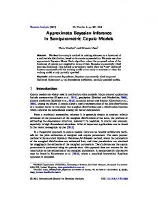
Results confirm that our SDN smoother consistently outperformed the others as it attained a better value for all of the metrics. The standard KS was incapable of estimating the state sequence. Its state estimation error was much larger than that of the other algorithms. The reason why the KS performed poorly is that the test rejected a large portion of the data—almost half, on average. The other algorithms, on the other hand, do not throw information away. Instead, they continuously adapt the noise and, in doing so, attain a lower state estimation error. Both the VB-AKF and the RS-SDN are the most accurate, owing to the fact that they are designed for correlated noise. Out of these two, the latter achieves higher trace correlation metrics because it tracks non-diagonal elements of the noise matrix. The reason why the KF-ROD and the RS-IID did not perform as well as the VB-AKF or the RS-SDN is that they regard the noise at different time stamps as being statistically independent, an assumption that does not hold in burst noise conditions. Fig. 3 shows a close-up on the first half of one of the 20 sets of data. In the upper plot, the first elements of the true state sequence are plotted as a solid black line. The grey band denotes the 99% confidence envelope for this first state, as estimated by the RS-SDN. Black dotted grid lines indicate the boundaries of the burst noise, i.e. a grid line at time step indicates . The true level of noise and the first element of the observed data appear in the middle and lower plots, respectively. The black line in the middle plot is the first diagonal element of , while the grey band is the estimated 99% confidence envelope. The sequence of measurements is drawn in black in the lower plot. From the figure we see that the data are infested with outliers. There are spurious observations that are more or less isolated from the rest, as well as continuous patches with an abnormally high level of noise contamination. There are also large spikes, which are markedly off, as well as smaller, less prominent ones of the same order magnitude as the nominal noise. Thus, for the standard KS it is difficult to disambiguate between correct measurements and outliers. In spite of the highly-variable and suddenly-changing noise, however, our model is able to track the states accurately and with high certainty. The upper plot in Fig. 3 shows how the confidence envelopes are slightly widened during periods of high contamination. This is because the level of noise inferred from the data determines the extent to which information is absorbed, and during a prolonged bout of outliers the uncertainty increases momentarily. Note that the true noise does not evolve smoothly, as the SDN model assumes. The brief intervals of steady, nominal noise are interrupted by periods of more intense variation. Still, even under incorrect assumptions, the middle plot shows, as do the correlation metrics in Table I, that the inferred noise follows the shape of the true noise.

5034


Fig. 3. Zoom-in on a 30-second interval from one of the 20 sets of data from the synthetic oscillator experiment. The upper plot shows the first hidden state in black, together with the 99% confidence envelope of the state as estimated by the RS-SDN in grey. The middle plot shows the true level of noise (black) of the first output, i.e. the first diagonal element of the posterior mean of the noise distribution, as well as the 99% confidence envelope of the corresponding noise estimates. The lower plot shows the observed data corresponding to the first input. Black dotted grid lines mark the regions of burst noise.

Algorithms 1 and 3 were implemented as MatLab scripts and run on an Intel Core Duo CPU with a 2.33 GHz processor and 4 Gb of RAM. Overall, fixed-interval smoothing for the IID noise and SDN models took 36.17 seconds, on average, per set of data. With a 1% termination tolerance for the loops, the algorithm typically required 3 (and never more than 6) iterations to converge. The most expensive routine, in terms of computation time, was the state update step, which amounted to an average of 2.257 milliseconds per time step. In contrast, each step of the noise backward pass took 0.213 milliseconds, a fraction of the time. We emphasize that line 21 of algorithm 3 was implemented in moment form and hence involved three matrix inversions; an information-form implementation would surely result in considerable computational savings, especially for higher-dimensional problems. B. Position Data In this experiment we tested our estimation algorithms on real data. The objective was to estimate the dynamic state of a mobile platform from measurements of its absolute position. A Segway sensor platform was mounted on the back of a utility car and driven for 20 min around a residential suburb. The platform was fitted with a NovAtel Global Positioning System (GPS) receiver and a Honeywell HG1700 Inertial Measurement Unit (IMU) as well as lasers and cameras. For this experiment, we recorded the position estimate from a NovAtel OEMV2 Synchronized Position Attitude Navigation (SPAN) system. The system returned the raw non-differential GPS readings at an average rate of 1 Hz as well as the IMU acceleration and gyroscopic measurements at an average frequency of 50 Hz. It also fused both modalities to produce a more accurate estimate of the position of the platform. Fig. 4 shows the trajectory of the vehicle superimposed on an aerial photograph of the area. A total of 1300 position data were logged. Each data point consists of a set of latitude, longitude and altitude values along with their corresponding uncertainty as estimated by the GPS receiver. Fig. 5 plots the uncertainty along the trajectory. The

Fig. 4. The trajectory followed by the platform, shown in blue, superimposed on an aerial photograph of the area.

root-mean-squared measurement uncertainty is slightly over 7.5 mts for the latitude and longitude and 22.4 mts for the altitude. There are frequent and sudden increases in uncertainty, possibly due to multi-path fading effects and a poor satellite geometry. As a result, the position data are highly contaminated with outliers. This can be seen in Fig. 6, which closes in on four areas with an elevated noise level that pose a challenge for the estimation algorithms. The trajectory returned by the SPAN system, estimated from the fused IMU and GPS data, is drawn in solid black; the sequence of measured longitude-latitude pairs are plotted as a grey dotted line. Lines overlap as the vehicle traverses the same path multiple times. We defined a constant-acceleration point-mass model for the vehicle dynamics. The velocity and the acceleration of the platform must be inferred from the only output that is directly ob-


5035

TABLE II PERFORMANCE METRICS FOR THE POSITION DATA SET

Fig. 5. Measurement uncertainty as provided by the global positioning system receiver. We did not make use of this information in our experiment.

Fig. 6. Zoom-in on different parts of the trajectory. The trajectory estimated by the SPAN system is a solid black line. Raw position data are plotted as a sequence of grey dots connected by solid traces.

servable: the GPS position. Mathematically, the model is expressed as follows,

and

, where each or block is a 3 3 matrix and is the sampling period. The parameters , and were fitted to the trajectory returned by the SPAN system. The harmonic mean of the noise prior (19) is time-varying; for each , the diagonal elements of are set to the square of the uncertainty estimates provided by the GPS receiver (see Fig. 5). We ran the standard KF, the KF-ROD of Ting et al. [9], [26] and algorithm 2 on the position data set. A 99% confidence validation gate threshold was implemented on the KF to mitigate the impact of outliers. A relatively broad prior was set for the noise in both the KF-ROD and algorithm 2 to reflect the fact that the level of contamination is high. Specifically, we selected and , both one over their minimum admissible values. No comparisons were made against neither the VB-AKF of Särkkä and Nummenmaa [27] nor algorithm 4

since the noise level varies too rapidly relative to the frequency at which the data are acquired. Table II summarizes the estimation results for each of the three models in terms of performance metrics. We regarded the SPAN trajectory as the ground truth position sequence and calculated the same set of state metrics we defined in Section IV-A, plus an additional metric pertaining to the inconsistency, or overconfidence of the filter. Namely, we defined NInc as the total number of inconsistent estimates, where an estimate is inconsistent if its 99% confidence ellipse does not contain the corresponding true position. No metrics were evaluated for the noise since the measurement uncertainty that the GPS receiver returns is not reliable enough to draw any meaningful conclusions. Except for the last row, all values in the table are in units of meters. The numerical results in Table II indicate that our RF-IID outperformed the standard KF and the KF-ROD in terms of both state estimation accuracy and consistency. The root mean squared and the maximum error, as well as the number of overconfident estimates, are smallest for our model. In relative terms, our RF-IID performed 40% and 70% better than the standard KF in terms of average and maximum errors, and was 20% more consistent. On the other hand, the KF-ROD was almost 10% less accurate, on average, than our algorithm and nearly 30% less in the worst case, while being 80% less consistent. These results suggest that stretching the noise covariance in all directions, instead of just scaling it, pays off even in this low-dimensional problem. The KF rejected a total of 30 data points as they failed the test. MatLab implementations of the KF, KF-ROD and RF-IID took, respectively, 0.47, 1.22 and 0.89 sec to execute, indicating that the computational burden of our algorithm is comparable to that of the other two. V. DISCUSSION AND CONCLUSION In this article we have introduced a novel approach for processing sequential data in situations where Gaussian noise assumptions are not applicable. In particular, our robust linear-Gaussian state-space models are especially suited for data corrupted with outliers as well as with correlated and non-Gaussian noise. Efficient inference algorithms were developed, based on straightforward modifications of standard RTS forward and backward recursions. Our approach extends other related and recently-developed ones in the literature. Our algorithms automatically deal with outliers and do not require any manual parameter tuning, heuristics or sampling. Experimental results with synthetic and real data have shown that our algorithms outperform the standard -based Kalman filter and the RTS smoother as well as recent, robust algorithms proposed in [9], [26] and [27].

5036


Let us summarize our contributions. In this paper we have: • Generalized the family of linear-Gaussian state-space models by allowing the measurement noise to be heavy-tailed and time-correlated; • Described this new family of models both qualitatively and quantitatively and proposed two specific instances of these models, namely the IID noise and SDN models; • Developed linear-time algorithms for performing approximate inference on both of these instances and shown the connection between these and other algorithms in the literature, including the classical KF and KS; We hope that our derivation of the approximate inference equations prompts colleagues to venture into other distributions beyond the Gaussian. We also hope our work encourages other researchers to apply these same ideas and incorporate them as building blocks of more complex models. We are currently looking into ways of extending our approach to the structured estimation setting. Specifically, we are studying how robust state-space models can be generalized to the relational framework, where some observations may be conditionally independent of others given the rest. Accounting for these conditional relationships has the potential to dramatically reduce the variance in the estimation of the noise, especially in situations with sparse dependencies, resulting in a much more confident state posterior. It also allows for domain knowledge to be seamlessly incorporated into the model, say in the form of an undirected graph. However, this requires us to alter the distributional assumptions placed on the noise model and develop richer and more flexible probability density functions over subset of the positive-definite cone. Preliminary results based on the hyper-inverse Wishart [59] and other alternative Wishart distributions [60] suggest that this is a promising direction for future research. ACKNOWLEDGMENT The authors would like to thank J. Underwood for his assistance during the process of collecting the data and L. Merry for her help with the navigation system. REFERENCES [1] B. Anderson and J. Moore, Optimal Filtering. Englewood Cliffs, NJ: Prentice-Hall, 1978. [2] R. Brown and P. Hwang, Introduction to Random Signals and Applied Kalman Filtering. New York: Wiley, 1991. [3] Y. Bar-Shalom, X. Li, and T. Kirubarajan, Estimation With Applications to Tracking and Navigation. New York: Wiley, 2001. [4] H. Durrant-Whyte and T. Bailey, “Simultaneous localization and mapping (SLAM): Part I the essential algorithms,” IEEE Robot. Autom. Mag., vol. 13, pp. 99–110, 2006. [5] R. Pearson, “Outliers in process modeling and identification,” IEEE Trans. Control Syst. Technol., vol. 10, no. 1, pp. 55–63, Jan. 2002. [6] F. Grubbs, “Procedures for detecting outlying observations in samples,” Technometrics, vol. 11, no. 1, pp. 1–31, Feb. 1969. [7] V. Barnett and T. Lewis, Outliers in Statistical Data. New York: Wiley, 1994. [8] J. Ting, A. D’Souza, and S. Schaal, “Automatic outlier detection: A Bayesian approach,” in Proc. IEEE Int. Conf. Robot. Autom., 2007. [9] J. Ting, E. Theodorou, and S. Schaal, “Learning an outlier-robust Kalman filter,” in Proc. 2007 Eur. Conf. Mach. Learn., 2007. [10] A. Jepson, D. Fleet, and T. El-Maraghi, “Robust on-line appearance models for visual tracking,” IEEE Trans. Pattern Anal. Mach. Intell., vol. 25, no. 10, pp. 1296–1311, Oct. 2003.

[11] J. Loxam and T. Drummond, “Student mixture filter for robust, realtime visual tracking,” in Proc. 10th Eur. Conf. Comput. Vis.: Part III, 2008. [12] T. Bailey and H. Durrant-Whyte, “Simultaneous localization and mapping (SLAM): Part II,” IEEE Robot. Autom. Mag., vol. 13, no. 3, pp. 108–117, Sep. 2006. [13] A. Gil, O. Reinoso, O. Mozos, C. Stachnissi, and W. Burgard, “Improving data association in vision-based SLAM,” in Proc. IEEE/RSJ Int. Conf. Intell. Robots Syst., Oct. 2006, pp. 2076–2081. [14] R. Kalman, “A new approach to linear filtering and prediction theory,” Trans. ASME J. Basic Eng., Series D, vol. 82, pp. 35–45, 1960. [15] R. Kalman and R. Bucy, “New results in linear filtering and prediction theory,” Trans. ASME J. Basic Eng., Series D, vol. 83, pp. 95–108, 1961. [16] S. Roweis and Z. Ghahramani, “A unifying review of linear-Gaussian models,” Neural Comput., vol. 11, no. 2, pp. 305–345, 1999. [17] R. Shumway and D. Stoffer, Time Series Analysis and Its Applications. New York: Springer-Verlag, 2005. [18] J. Morris, “The Kalman filter: A robust estimator for some classes of linear quadratic problems,” IEEE Trans. Inf. Theory, vol. 22, no. 5, pp. 526–534, Sep. 1976. [19] P. Huber, “Robust estimation of a location parameter,” Annals Math. Statist., vol. 35, no. 1, pp. 73–101, 1964. [20] H. Sorenson and A. Stubberud, “Non-linear filtering by approximation of the posterior density,” Int. J. Contr., vol. 8, no. 1, pp. 33–51, 1968. [21] H. Sorenson and D. Alspach, “Recursive Bayesian estimation using Gaussian sums,” Automatica, vol. 7, no. 4, pp. 465–479, 1971. [22] P. Szablowski, “Elliptically-contoured random variables and their application to the extension of the Kalman filter,” Comput. Math. With Appl., vol. 19, no. 2, pp. 61–72, 1990. [23] F. Girón and J. Rojano, “Bayesian Kalman filtering with ellipticallycontoured errors,” Biometrika, vol. 81, no. 2, pp. 390–395, Jun. 1994. [24] R. Meinhold and N. Singpurwalla, “Robustification of Kalman filter models,” J. Amer. Statist. Assoc., pp. 479–486, 1989. [25] I. Arasaratnam and S. Haykin, “Cubature Kalman filters,” IEEE Trans. Autom. Control, vol. 54, no. 6, pp. 1254–1269, Jun. 2009. [26] J. Ting, E. Theodorou, and S. Schaal, “A Kalman filter for robust outlier detection,” in Proc. IEEE Int. Conf. Intell. Robots Syst., 2007. [27] S. Sarkka and A. Nummenmaa, “Recursive noise adaptive Kalman filtering by variational Bayesian approximations,” IEEE Trans. Autom. Control, vol. 54, no. 3, pp. 596–600, Mar. 2009. [28] G. Agamennoni, J. Nieto, and E. Nebot, “An outlier-robust Kalman filter,” in Proc. IEEE Int. Conf. Robot. Autom., 2011. [29] M. Beal, “Variational algorithms for approximate Bayesian inference,” Ph.D. dissertation, Gatsby Computational Neuroscience Unit, Univ. College, London, U.K., 2003. [30] A. Doucet, S. Godsill, and C. Andrieu, “On sequential Monte Carlo sampling methods for Bayesian filtering,” Dept. Eng., Cambridge Univ., Tech. Rep. CUED/F-INFENG/TR310, 1998. [31] A. Doucet, N. De Freitas, and N. Gordon, Sequential Monte Carlo Methods in Practice. New York: Springer-Verlag, 2001. [32] N. Lawrence, “Variational inference in probabilistic models,” Ph.D. dissertation, Univ. Cambridge Computer Lab., Cambridge, U.K., 2000. [33] M. Grewal and A. Andrews, Kalman Filtering: Theory and Practice. Englewood Cliffs, NJ: Prentice-Hall, 1993. [34] A. Dawid, “Some matrix-variate distribution theory: Notational considerations and a Bayesian application,” Biometrika, vol. 68, pp. 265–274, 1981. [35] R. Muirhead, Aspects of Multivariate Statistical Theory. New York: Wiley, 1982. [36] P. Diaconis and D. Ylvisaker, “Conjugate priors for exponential families,” Annal. Statist., vol. 7, no. 2, pp. 269–281, 1979. [37] J. Wishart, “The generalized product moment distribution in samples from a normal multivariate population,” Biometrika, vol. 20A, no. 1, pp. 32–52, Jul. 1928. [38] M. Abramowitz and I. Stegun, Handbook of Mathematical Functions, With Formulas, Graphs and Mathematical Tables. New York: Dover, 1974. [39] W. Gosset, “The probable error of a mean,” Biometrika, vol. 6, no. 1, pp. 1–25, 1908. [40] S. Kotz and S. Nadarajah, Multivariate Distributions and Their Applications. Cambridge, U.K.: Cambridge Univ. Press, 2004. [41] F. Hampel, E. Ronchetti, P. Rousseeuw, and W. Stahel, Robust Statistics: The Approach Based on Influence Functions. New York: Wiley, Mar. 1986. [42] J. Jensen, “Sur les fonctions convexes et les inégalités entre les valeurs moyennes,” Acta Mathematica, vol. 30, no. 1, pp. 175–193, Dec. 1906.


[43] A. O’Hagan, “A moment of indecision,” Biometrika, vol. 68, no. 1, pp. 329–330, 1981. [44] J. Drèze, “Bayesian regression analysis using poly- densities,” J. Econometr., vol. 6, no. 3, pp. 329–354, Nov. 1977. [45] R. Neal and G. Hinton, “A view of the EM algorithm that justifies incremental, sparse, and other variants,” in Proc. NATO Adv. Study Inst. Learn. Graphical Models, M. Jordan, Ed., 1998. [46] S. Kullback and R. Leibler, “On information and sufficiency,” Annal. Math. Statist., vol. 22, no. 1, pp. 79–86, 1951. [47] P. Naveau, M. Genton, and X. Shen, “A skewed Kalman filter,” J. Multivariate Anal., vol. 94, no. 2, pp. 382–400, Jun. 2005. [48] R. Bucy and P. Joseph, “Filtering for stochastic processes with applications to guidance,” in Proc. Amer. Math. Soc. Chelsea, 2005. [49] S. Julier and J. Uhlmann, “A new extension of the Kalman filter to nonlinear systems,” in Proc. Int. Symp. Aerospace Defense Sensing, Simulation, Contr., 1997. [50] M. Verhaegen and P. Van Dooren, “Numerical aspects of different Kalman filter implementations,” IEEE Trans. Autom. Control, vol. 31, no. 10, pp. 907–917, Oct. 1986. [51] P. Park and T. Kailath, “New square-root smoothing algorithms,” IEEE Trans. Autom. Control, vol. 41, no. 5, pp. 727–732, May 1996. [52] H. Akaike, “A new look at the statistical model identification,” IEEE Trans. Autom.Control, vol. 19, no. 6, pp. 716–723, Dec. 1974. [53] G. Schwarz, “Estimating the dimension of a model,” Annal. Statist., vol. 6, no. 2, pp. 461–464, 1978. [54] F. Liu, “Bayesian time series: Analysis methods using simulation-based computation,” Ph.D. dissertation, Inst. Statist. Decision Sci., Graduate School of Duke Univ., Durham, NC, 2000. [55] C. Carvalho and M. West, “Dynamic matrix-variate graphical models,” Bayesian Anal., vol. 2, no. 1, pp. 69–98, 2007. [56] K. Murphy, Switching Kalman Filters Univ. California, Berkeley, CA, Compaq Cambridge Res. Lab. Tech. Rep. 98-10, 1998. [57] Z. Ghahramani and G. Hinton, “Variational learning for switching state-space models,” Neural Comput., vol. 12, no. 4, pp. 831–864, 2000. [58] D. Barber, “Expectation correction for smoothed inference in switching linear dynamical systems,” J. Mach. Learn. Res., vol. 7, pp. 2515–2540, Dec. 2006. [59] A. Roverato, “Cholesky decomposition of a hyper-inverse Wishart matrix,” Biometrika, vol. 87, no. 1, pp. 99–112, 2000. [60] G. Letac and H. Massam, “Wishart distributions for decomposable graphs,” Annal. Statist., vol. 35, no. 3, pp. 1278–1323, 2007.

5037

Gabriel Agamennoni (M’11) received the B.Sc. degree in electronic engineering from the Universidad Nacional del Sur, Argentina. He is currently working toward the Ph.D. degree at the Australian Centre for Field Robotics, University of Sydney, Sydney, Australia. His research interests include statistical modeling and machine learning.

Juan I. Nieto received the Ph.D. in robotics at the University of Sydney, Sydney, Australia, in 2005. Until 2007, he was a Research Associate at the Australian Centre for Field Robotics. From 2007, he has been a Senior Research Fellow at the Rio Tinto Centre for Mine Automation, University of Sydney, Sydney, Australia. He has over 50 publications in international journals and conferences. His main research interests include navigation systems and perception.

Eduardo M. Nebot (S’79–M’81–SM’01) received the BSc. degree in electrical engineering from the Universidad Nacional del Sur, Argentina, and the M.Sc. and Ph.D. degrees from California State University, Long Beach, CA. He is currently a Professor at the University of Sydney, Sydney, Australia, and the Director of the Australian Centre for Field Robotics. His main research interests are field robotics automation. The major impact of his fundamental research is in autonomous system, navigation, and mining safety.