function and the distribution of costs in constraints, thus allowing us to ..... our model approximates the true cumulative probability distribution function of the total ...
Approximate Probabilistic Constraints and Risk-Sensitive Optimization Criteria in Markov Decision Processes Dmitri A. Dolgov and Edmund H. Durfee Department of Electrical Engineering and Computer Science University of Michigan Ann Arbor, MI 48109 ddolgov,durfee�@umich.edu Abstract The majority of the work in the area of Markov decision processes has focused on expected values of rewards in the objective function and expected costs in the constraints. Although several methods have been proposed to model risksensitive utility functions and constraints, they are only applicable to certain classes of utility functions and allow limited expressiveness in the constraints. We propose a construction that extends the standard linear programming formulation of MDPs by augmenting it with additional optimization variables, which allows us to compute the higher order moments of the total costs (and/or reward). This greatly increases the expressive power of the model, and supports reasoning about the probability distributions of the total costs (reward). Consequently, this allows us to formulate more interesting constraints and to model a wide range of utility functions. In particular, in this work we show how to formulate the constraint that bounds the probability of the total incurred costs falling within a given range. Constraints of that type arise, for example, when one needs to bound the probability of overutilizing a consumable resource. Our construction, which greatly increases the expressive power of our model, unfortunately comes at the cost of significantly increasing the size and the complexity of the optimization program. On the other hand, it allows one to choose how many higher order moments of the costs (and/or reward) are modeled as a means of balancing accuracy against computational effort.
1 Introduction Markov processes are widely used to model stochastic environments, due to their expressiveness and analytical tractability. In particular, unconstrained (e.g. [3, 4, 8, 15]) as well as constrained (e.g. [1, 2]) Markov decision processes have gained significant popularity in the AI and OR communities as tools for devising optimal policies under uncertainty. The vast majority of the work in the area has focused on optimization criteria and constraints that are based on the expected values of the rewards and costs. However, such risk-neutral approaches are not always applicable and expressive enough, 1 thus precipitating the need for extending the MDP framework to model risk-sensitive utility functions and constraints. Several approaches [9, 12, 13] to modeling risk-sensitive utility functions have been proposed that work by transforming risk-sensitive problems into equivalent risk-neutral problems, which can then be solved by dynamic programming. However, this transformation only works for a certain class of utility functions. Namely, this has been done for exponential utility functions that are characteristic of agents that have “constant local risk aversion” [14] or obey the “delta property” [9], which says that a decision maker’s risk sensitivity is independent of his current wealth. This approximation has a number of very nice analytical properties, but is generally considered somewhat unrealistic [9]. Our work attempts to address this issue via approximate modeling of a more general class of utility functions. As with utility functions, there has been a significant amount of work on risk-sensitive constraints in MDPs. These methods typically work by constraining or including in the objective function the variance of the costs [6, 7, 10, 18, 19] or reasoning about sample-path costs in the case of per unit-time problem formulations [2, 16, 17]. However, in some cases, reasoning about the variance only is also not expressive enough (see [5] for a more detailed discussion). We propose a method that allows explicit reasoning about the probability distributions of the total reward in the objective function and the distribution of costs in constraints, thus allowing us to represent a wide class of interesting optimization criteria and constraints. In this work, we describe a method for handling probabilistic constraints, but the approach is also directly applicable to risk-sensitive objective functions. We focus on transient (or episodic) Markov processes [11] and 1 As
pointed out, for example, by Ross and Chen in the telecommunication domain [16].
1
base our approach on the standard occupancy-measure linear programming formulation of constrained Markov decision processes (CMDPs). We augment the classical program with additional optimization variables, which allows us to compute the higher order moments of the total incurred costs for stationary Markov policies. This enables us to reason about the probability distributions of the total costs, and consequently, to express more interesting constraints such as bounding the probability that the total costs fall within a given range (or exceed a threshold). It is important to note that, in general, arbitrary utility functions and arbitrary constraints do not obey the Markov property, which means that stationary Markov (history-independent) policies are not guaranteed to be optimal under such utility functions and constraints. However, given the practical difficulty of implementing non stationary history-dependent policies, in this work we limit the search to the class of stationary Markov policies, i.e. we are interested in finding the best policy that satisfies the given constraints and maximizes the given utility function, among the class of stationary historyindependent policies.
2 Preliminaries We formulate our optimization problem as a stationary, discrete-time, fully-observable constrained Markov decision process. In this section, we review some well-known facts from the theory of standard [3, 15] and constrained [1] fullyobservable Markov decision processes. � ��, where � is a finite A standard constrained Markov decision process (CMDP) can be defined as a tuple � � set of states, � is a finite set of actions, ���� � � � � � � � � �� �� defines the transition function (� �� is the probability �� � � � � � �� �� is the initial probability distribution that the agent will go to state � if it executes action � in state �), over the state space, � �� � � � � � � � � defines the reward function (agent receives a reward of � � for executing action � in state �), and � ��� � � � � � are the costs.2 A solution to a CMDP is a policy that prescribes a procedure for selecting an action that typically maximizes some measure of performance (based on the rewards �), while satisfying constraints (based on the costs �). A stationary Markov policy � can be described as a mapping of states to probability distributions over actions: � �� � � � � � � � �� ��. We address the problem of finding optimal stationary Markov policies, under probabilistic constraints (defined in section 3). For a Markov system, the initial probability distribution , the transition probabilities, and the policy together completely determine the evolution of the system in a stochastic sense:
�� � ��
�� � ����
(1)
where �� � � � � �� is the probability distribution of the system at time , and ��� ���� � is the probability � �� ��� ). transition matrix induced by the policy ( ��� In this work we focus our attention on discrete-time transient (or episodic) problems, where there is no predefined number of time steps that the agent spends in the system, but it cannot stay there forever. Given a finite state space, this � assumption implies that there have to exist some state-action pairs �� �� for which � ��� � �. the analysis in this paper we use the expected total reward as the policy evaluation criterion: �� � � For�most of �
� � � �� �� , which, for a transient system with bounded rewards, converges to a finite value. � � � A standard CMDP where constraints are imposed on the expected total costs, and the expected total reward is being maximized can be formulated as the following linear program [1, 15]:
�
�� �
� ��
� � � � � �
�
�
�
��
� �
�
�
�
� ���
�
�
��
�
�
(2)
where �� is the upper bound on the expected total incurred cost, and the optimization variables � are called the occupancy measure of a policy and be interpreted as the expected total number of times action � is executed in state �.
3 Problem Description Given a standard constrained MDP model � � � ��, we would like to find a policy that maximizes the total expected reward, while satisfying the constraints on the probability of that the cost exceed a given upper bound, i.e. � �� � � � � �� , 2 The costs are said to be incurred for visiting states rather than executing actions, but all results can be trivially extended to the latter case. Also note that most interesting problems involve several costs, and while we make the simplification that there is only one cost incurred for visiting a state, this is done purely for notational brevity. All results presented in this work are directly applicable (and most useful) for problems with several costs.
2
where � is the total cost. In other words, we need to solve the following optimization problem:
�
��
�� �
�
� � � � �
� � � � � �� � �� � ��
� ���
��
(3)
where the optimization variables � have the standard interpretation of the expected total number of times action � is executed in state �. If � �� � � � � could be expressed as a simple function of � � � �, the problem would be solved, as one could simply plug the expression into the above program. Unfortunately, things are not as wonderful, and the above dependency is significantly more complex. A simple linear approximation to the above program (when costs are non-negative) can be obtained by using the Markov inequality:
�
� �
�
��
�
� �
�
� �
�
� �
�
�
�
��
�
(4)
�
which allows one to express � �� � � � � as a linear function of the occupancy measure �. Our investigation [5] of this approximation showed, unsurprisingly, that this linear approximation is computationally cheap but usually leads to suboptimal policies, because the Markov inequality provides a very rough upper bound on the probability that the total cost exceed a given limit � � . The purpose of this work is to improve this approximation. To this end, we are going to come up with a system of coordinates �, such that the constraint � �� � � � � �� can be expressed as a simple function of �, so that the expression can be plugged into the optimization program (eq. 3). However, one has to note that there are only � � free parameters in the system, so not all optimization variables � are going to be independent and additional constraints might have to be imposed. As mentioned earlier, the method presented in this paper works for more general problems than (eq. 3), which we use as an interesting example to illustrate the approach. Section 7 comments on other problems that this method applies to.
4 Calculating the Probability of Exceeding Cost Bounds To find the probability of exceeding the cost bounds, it would be very helpful to know the probability density � function (pdf) 3 �� �� �. Then, the probability of exceeding the cost bounds could be expressed simply as � �� � � � � �¼ �� �� ���� Unfortunately, � � �� � is not easily available. However, it is a well-known fact that under some conditions the moments of a random variable� completely specify its distribution. 4 The � th moment of a random variable is defined as the expected value of � : ��� � �� � � � � � One way to compute the pdf � � � �, given the moments � �� is via an inverse Legendre
� � � � transform.5 Indeed, the Legendre polynomials � � � � �� �� � �� form a complete orthogonal set on the interval �� � � � ��: �� � ���� � ��Therefore, a function on that interval � � �� can be approximated as a weighted sum of th Legendre polynomials: � � � � � �� � � � where � � � is the � Legendre polynomial, and � � is a constant coefficient, obtained by multiplying the polynomials by � � �, integrating over � � ��, and using the orthogonality condition: ��
Realizing that
�
� � � � �
�
�
� � � � � � � � � �� �
�
�
�
�
�
(5)
��� ��
is just a linear combination of several moments � �� , we get:
��
��
�
�
�
�
��
�
��� �� �
(6)
where in the second summation, the index � runs over all powers of present in � . Therefore, for an express the probability that is greater than some � as a linear function of the moments:
�
�
�
��
� � �¼
��
�� �
� ��� �¼ �
�
�
�
��
��� �� � �
� �
� ��
��
�
��
� � ��, we can
�
(7)
3 Note that, in general, for an MDP with finite state and action spaces, the total costs have a discrete distribution. However, we make no assumptions about the continuity of the pdf � �, and our analysis carries through for both continuous and discrete density functions; in the latter case, � � can be represented as a sum of Dirac delta functions: � � � � �� Æ � �� �. 4 This is true when the power series of the moments that specifies the characteristic function converges, which holds in our case due to the transient nature of the Markov process and the fact that costs are finite. 5 A more common and natural way involves inverting the characteristic function of � via a Fourier transform, but the method does not work for this problem.
�
3
�
��
th where �� � � � � ��� �¼ � � �� , in which the index � runs over all polynomials that include the � power of . Therefore, if we normalize � to be in the interval � � �� (section 6 discusses in more detail the necessary transformation �. for a transient system), we could use the above method to express � �� � � � � as a linear function of the moments � � � Now, if we could come up with a system of coordinates �, such that the moments � � could be expressed via �, we might be able to formulate a manageable approximation to (eq. 3). However, it is important to note that unless we use an infinite number of moments, the resulting program will be an approximation to the original one.
5 Computing the Moments As mentioned in the previous section, the properties of the pdf of the total cost are not immediately obvious, as the total cost is a sum of a random number of dependent random variables. We do, however, know how the system evolves with time, i.e. given the initial probability distribution, a policy, and the corresponding transition probabilities over states, we ��� ���� � is the probability know the probability that the system is in state � at time – it is simply � � ��� , where � �� ��� ). In other words, we know the probability distribution for the transition matrix induced by the policy ( ��� random variables � � � � �� ��, where �� � � � if state � is visited at time , and 0 otherwise. � Let us also define for every state a random variable � � � � �� � � that specifies the total number of times state � is � of � can be expressed as linear functions of the cross-moments � ��½ ��¾ � � � ��� � visited. Then, the moments � � �½
�� (the expected value of the product) as follows:
�
�
��
�
��
�
��
�
�� �� �
�
�� ��
��
�
��
��
�
�
�½
�¾
��
�
Let us now compute the first moments � � its mean equals the probability that � � � � is 1:6
�
��
�
where � is the identity matrix, and Multiplying by �� �, we get:
�
� �
�
�
��½ ��¾
�� �
�
�� �� ���
�
�
�
�
� ��. Recalling that � � �
�
�
��
�
�
�� ��
�
� ��, and, therefore,
�
�� ��� ��� ��
�
(9)
�� ��� holds, because � �� ��
(8)
� � � ��� ��½ �¾
��
�
� � ��
� ��
�� ��
�� �� �� �� �
� �� � ��
�
�
�
�
��
�
���
�
�� �� �
� for our transient system.
�
(10)
��
Note that the above is exactly the “conservation of probability” constraint in (eq. 3). Indeed, since
� �� �� , the two are identical. Let us now compute the second moments in a similar fashion: ���
�� �
�� �� �
� � �½
� �¾
�½
�½
�
�� �
� ��
��
�¾
� � � � � � �� �
��
�
�
�
� �
�¾
��
� ��
��
� �½
�¾
� � � � � � ��
��
�
�
��� ��
and
� � � � � � ��
��
� �¾ �
�½
���
�
�
�
�
� � � ��
(11)
�� ��
Once again recalling that � � � � are binary variables, and since the system can only be in one state at a particular time, the mean of their product is:
� � � � � � ��
��
6 Hereafter
�
� � � � � � � �� �� � � � � ��
� �� Æ
� �
�
if � if � �
� �
we use the notation � ��� for binary variables as a shorthand for � �� � ��, and � ��� � � for � � � � ��
4
(12)
�
�
� ���
where � ��� � � � �� � � �� is the probability that state � is visited at time � and state system is Markovian, for � � , we have: �
is visited at time � . Also, since the
� � � � � � � �� � � � � �� � �¾ ��½ ��� � � � � ��
� � � � � � � ��
� ��
�
� ��
�
� �
�
� �
(13)
Substituting, we obtain:
� �
���
�½
�½
�
� �¾
�
�
� � �¾ ��½ ��� � � � � �� �
�½
� �
�¾
�
�
� � � �� � ����� � �¾ �� � � � � � ��� � � �� ��� �
� ��
��
�
�
�
�
�
� �½
� � �½ ��¾ ��� � � � � �� �
�¾
� � � ��
� ��
� �
�
�
�
� � � ��
�� � ��
�� ��� �� � � ��� � � �� � � �� �
�
�
(14)
�� ��
Unfortunately, as can be seen from the above expression, the second moments cannot be tied to the first moments via a linear function. Therefore, we cannot use the moments as the optimization variables directly. Instead, we are going to work with the following asymmetric terms where the order of indexes of � corresponds to an temporal ordering of the terms in the sums:
�
��
�
��½ �¾
��
�
� �
���
�½
½ ��
�
� ��
��
� �¾
��½
��
�
��
�� ����� � �
� � � � � � �� �½ �� � ½ �� �� ��
�
½
�
�½
� �¾
�½
� � � � � � � �� � � � � ��
� ��
�
� �
��
�� �����
(15)
�
We will refer to the above terms as the asymmetric moments (although they do not correspond to moments of any real variables). Clearly, all of the � th order asymmetric moments can be expressed as a linear function of the asymmetric moments of order � � by moving the �� � term to the left-hand side. For example, for the second moments this step can be easily done by rewriting (eq. 15) in matrix form:
��� �� � ��� ���
(16)
�
where ��� ���� � is the matrix of second order asymmetric moments, and ��� � � is a diagonal matrix, with values of the ���� �. Similarly, for first order moment � � on the diagonal. Multiplying by �� � on the right, we get � �� ��� the other moments we get: ��
���
� �
�� ���
� �
��½ �¾
��
��
��� ���
½ ��
� �
�� ��
(17)
��½ �¾
��
½ ��� ½ �
Æ�½ �� ��½ �¾
��
½
Furthermore, it can be seen that the true moments of order � can be expressed as linear functions of the asymmetric moments of orders 1 through � : �� ����
�� ����
���
�
�� ���
����
���
�
�
���
����
�� ���
�
�
�� ��
����
�
����
�
����
�� ��� �� ��� �� ��� �� ���
(18)
��� ��
Indeed, for the first moments, there is only one state index and therefore the first asymmetric moment equals the � ), and thus we have to subtract true For the second moments, both � �� and ��� include the term ( � � � moment. �� � � ��� � � �� Æ�� �� . The expressions for other moments are obtained in a similar manner. �¾ �½ �½ 5
� The last step that remains in formulating the optimization program is to substitute the transition probabilities
���
and to define the actual optimization variables. This is where we hit a problem that breaks the linearity of the �� �� �� �� and have the program. Recall that for the standard CMDP, the optimization variables are defined as � interpretation of the expected total number of times action � is executed in state �. As mentioned earlier, this allows one to � express the first-order constraint from (eq. 17) as a linear function of
� . Indeed, since �� � , the first moments are �
� , and recalling that � �� �� �� �� , we have for the first order constraint: simply �� ��� ��
��
� �
�� ���
�
�
� �
��
�
�
��� ��
�
�� �
��� �
(19)
Unfortunately, the same trick does not work for the higher order constraints. If we were to define similar variables for the higher-order moments (ex. �� ��� �� ), we could, of course, rewrite (eq. 17) as linear functions of these variables. However, by doing this, we would introduce too many free parameters into the program. To retain the original desired interpretation of the variables, we would also have to add constraints to ensure that the policy � implied by the higher-order variables is the same as the one computed from the first-order � . Clearly, these new constraints would be quadratic:
�
½
��
½
�
¾
��
¾
���
��
½
��
¾
(20)
Hence, it appears that there is no easy way to avoid the quadratic expressions (� �� �� ) in the constraints on the moments:
�
���
�
����
� �
�
�
� ���
�
��½ �¾
��
�� �
��
�
����
½ ��
� ���
��� ��
�
� �
��
��� ��
��½ �¾
��
�� ��
(21)
�� ���
� ½
��
�
½�
���
½
Æ�½ �� ��½ �¾
��
½
�
�� �
We are therefore left with�an� optimization program in � and the asymmetric moments (� �� ��� ���� � � �) that has: a linear objective function �
� �� , a constraint on the probability of the total cost exceeding a given threshold, which is linear in the moments � (eq. 7), which are linear in � (eq. 18), and a system of quadratic constraints that synchronizes the moments (eq. 21).
6 An Example As an example of the use of the method presented in the previous sections, let us consider a toy problem, for which we can analytically compute the distribution of the total cost, and formulate a constrained optimization program for it using the first three moments of the total cost. In this section we present a more careful derivation of the optimization program, paying more attention to some steps that were just briefly described in section 4. We also present a preliminary empirical analysis that shows how closely our model approximates the true cumulative probability distribution function of the total cost. The purpose of the latter is to serve as a rough indication of the accuracy of our approach, which we cannot yet directly report on, as at the time of writing we do not have the optimization implemented yet. Consider the problem depicted in figure 1(a). In this problem, there are two states, one of which (� ) is a sink state. If the agent starts in state 1 ( �� ��), the total received reward is the same as the total incurred cost, and both equal the total number of visits to state 1. The obvious optimal policy for the unconstrained problem is to always execute action 1 in �� � � ��). If we set the upper bound on the cost as � � ��, the unconstrained optimal policy has about a state 1 (� 30% chance of exceeding that bound. As we decrease the acceptable probability of exceeding the cost bound, the policies should become more conservative, i.e. they should prescribe higher probabilities of executing action 2 in state 1. In order to apply the Legendre approximation from section 4, one has to ensure that the total cost � is in the range � � ��. Clearly, this is not generally the case for our problem. Therefore, to satisfy this condition, we apply a transformation
6
F�S� 1
a1: p111=0.9, r11=1
Error �Legendre 3�
cdf �real & Legendre 3�
0.1
0.8
a1: p112=0.1, r11=0
0.6
c1=1
c2=0
S
�0.5 real
0
0.5
1
�0.1
Legendre 3 0.4
a2: p212=1.0, r12=0
�0.2
0.2
�0.3 �0.5
0
(a)
0.5
1
S
�0.4
(b)
(c)
Figure 1: (a) – simple problem with two states and two actions; (b) – the actual cdf of the total cost and the cdf computed from a third-degree Lagrange approximation of the pdf of the cost; (c) – relative error of the approximation in (b).
��� � � with � � �� (a reasonable approximation, as � �� � ��� �����). 7 Figure 1(b) shows the resulting cumulative distribution function � � �� � for the unconstrained optimal policy and the cdf computed from a third-degree approximation of the pdf � �� �. Figure 1(c) shows the relative error of the third-degree approximation and serves to show that we can expect to get a reasonably good approximation of the cdf using just the first three moments. Note that the pdf for this problem is discrete (thus, harder to approximate with continuous Legendre polynomials), but we can still get a reasonably good approximation of the cdf, which is what we really care about, as our goal is to estimate � �� � � � � � �� ��� �. Let us now compute a third-order approximation to � � �� � for an arbitrary policy by computing the coefficients � � (eq. 5): �
� � � �� � � � � �� � (22) � � � � � � � � � Notice that here we have to use the moments of � � � ��. However, the constraints in (eq. 21) operate on moments , and since our optimization variables are going to be the moments of � �� � �, we have to be able to express the �
�
�
�
�
�
��
�
�
��
�
�
�
�
�
�
�
�
�
of � � � former via the latter. This can be easily done by solving the following linear system of equations for � � :
�
�
����
� �
�� � ��
�
� �
�
�
� �
�� � ��
�
�
�
� ��
�� � � � � � � � �� � � � � � � � � � � Now, the probability of exceeding the cost bounds is simply � � where � � � �. ��
� �
�
� �
� �
�� � � � � �
� �
�
�
�
�
� �
�
� �
�
�
��
� ��
� �
�
� ����
�� � � �� � � �� � � � � � �
�
� �
�� � ��
�¼
�
�
(23)
�
��
��
�¼ ��
� �
� ��
� ��
7 Conclusions In this paper we have introduced a method for approximately reasoning about the probability distributions of rewards and costs in Markov decision processes. The main three sources of approximation error in our method are: 1) the use of Legendre polynomials to approximate the true pdf, 2) the use of a finite number of moments (the more moments are used, the better � the approximation), and 3) truncation of the costs at some upper bound � � (the lower the mass of the remaining cost ���� � �� �� �, the better the approximation). We demonstrated the approach on a specific problem that bounds the probability that the total cost exceeds a given upper bound. However, it is easy to see that the method allows one to model a wide range of risk-sensitive objective functions and constraints. Indeed, one can just as easily approximate the distribution of the total (normalized) reward and express the expected value of the utility function as (similarly to (eq. 7)):
� � ��
�
� �
�� �� �� �� � � � � � � �
� � � �
�
�
�
� � ��
�� �
�
�
�
��� � �
� � � � �
�
�
�
�
!� �
(24)
� � , �� � is the utility of getting reward , and � � � is the distribution of the total where !� �� reward. Then, the approximation methods of sections 4 and 5 are directly applicable. Of course, the above relies on the fact
7 For a transient system with bounded rewards ��� ¼ � �� � ���� � is arbitrary small.
� � �� � �¼ � � . Thus one can always compute or estimate a reasonable ���� for which 7
that there either exists a natural upper bound on the largest possible utility value of a policy, or that there exists an upper �� bound � such that the weighted tail of the utility distribution ��� � � ��� �� is sufficiently small. Even though our construction yields more complex optimization programs than the standard constrained MDP approach, it is more expressive than the standard risk-neutral CMDP techniques, because our formulation allows one to reason about the probability distributions instead of the expected values of the total cost and rewards. Our ongoing efforts in extending this work include several directions such as looking at ways of efficiently encoding and implementing the optimization program, more careful investigation of the complexity and convergence properties of the model (as more moments are used), exploring heuristics for choosing an appropriate number of moments, and a formal analysis of properties of the problem and the corresponding solutions. Acknowledgments This work was supported by DARPA and the Air Force Research Laboratory under contract F3060200-C-0017 as a subcontractor through Honeywell Laboratories and also by Honeywell Laboratories through the “Industrial Partners of CSE” program at the University of Michigan. The authors thank the anonymous reviewers for their comments.
References [1] E. Altman. Constrained Markov Decision Processes. Chapman and HALL/CRC, 1999. [2] E. Altman and A. Shwartz. Adaptive control of constrained Markov chains: Criteria and policies. Annals of Operations Research, special issue on Markov Decision Processes, 28:101–134, 1991. [3] C. Boutilier, T. Dean, and S. Hanks. Decision-theoretic planning: Structural assumptions and computational leverage. Journal of Artificial Intelligence Research, 11:1–94, 1999. [4] T. Dean and M. Wellman. Planning and Control. Morgan Kaufmann, 1991. [5] D. A. Dolgov and E. H. Durfee. Approximating optimal policies for agents with limited execution resources. In Proceedings of the Eighteenth International Joint Conference on Artificial Intelligence, pages 1107–1112, 2003. [6] J. A. Filar and L. C. M. Kallenberg. Variance-penalized markov decision processes. Math. of OR, 14:147–161, 1989. [7] J. A. Filar and H. M. Lee. Gain/variability tradeoffs in undiscounted markov decision processes. In Proceedings of 24th Conference on Decision and Control IEEE, pages 1106–1112, 1985. [8] R. Howard. Dynamic Programming and Markov Processes. MIT Press, Cambridge, 1960. [9] R. Howard and J. Matheson. Risk-sensitive markov decision processes. Management Science, 18(7):356–369, 1972. [10] Y. Huang and L. Kallenberg. On finding optimal policies for Markov decision chains. Math. of OR, 19:434–448, 1994. [11] L. Kallenberg. Linear Programming and Finite Markovian Control Problems. Math. Centrum, Amsterdam, 1983. [12] S. Koenig and R. G. Simmons. Risk-sensitive planning with probabilistic decision graphs. In J. Doyle, E. Sandewall, and P. Torasso, editors, KR’94: Principles of Knowledge Representation and Reasoning, pages 363–373. Morgan Kaufmann, San Francisco, California, 1994. [13] S. Marcus, E. Fernandez-Gaucherand, D. Hernandez-Hernandez, S. Colaruppi, and P. Fard. Risk-sensitive markov decision processes, 1997. [14] J. Pratt. Risk aversion in the small and in the large. Econometrica, 32(1-2):122–136, 1964. [15] M. L. Puterman. Markov Decision Processes. John Wiley & Sons, New York, 1994. [16] K. Ross and B. Chen. Optimal scheduling of interactive and non-interactive traffic in telecommunication systems. IEEE Transactions on Auto Control, 33:261–267, 1988. [17] K. Ross and R. Varadarajan. Multichain Markov decision processes with a sample path constraint: A decomposition approach. Math. of Operations Research, 16:195–207, 1991. [18] M. Sobel. Maximal mean/standard deviation ratio in undiscounted mdp. OR Letters, 4:157–188, 1985. [19] D. J. White. A mathematical programming approach to a problem in variance penalised markov decision processes. OR Spectrum, 15:225–230, 1994.
8