APPROXIMATE SOLUTION OF BOUNDARY VALUE ... - ijpam

International Journal of Pure and Applied Mathematics Volume 114 No. 4 2017, 823-833 ISSN: 1311-8080 (printed version); ISSN: 1314-3395 (on-line version) url: http://www.ijpam.eu doi: 10.12732/ijpam.v114i4.12

AP ijpam.eu

APPROXIMATE SOLUTION OF BOUNDARY VALUE PROBLEM WITH BERNSTEIN POLYNOMIAL LAPLACE DECOMPOSITION METHOD Dimple Rani1 , Vinod Mishra2 § 1,2 Department

of Mathematics Sant Longowal Institute of Engineering and Technology Longowal, 148106, INDIA Abstract: In this paper, a new approach enabling Laplace Adomian decomposition method in combination with Bernstein polynomials for numerical solution of boundary value problem is introduced. The accuracy of the method is dependent on the size of the set of Bernstein polynomials. Numerical results with comparisons are given to establish the reliability of the proposed method for solving singular and nonsingular boundary value problem. Convergence analysis of the presented technique is also discussed. AMS Subject Classification: 41A10, 44A10, 35G30, 49M27 Key Words: Laplace Adomian decomposition method, Bernstein polynomials, singular and nonsingular boundary value problem

1. Introduction Nonlinear boundary value problems (BVPs) eminently emerge in the modelling of real life problems. A huge research has been conducted to find the numerical solutions of these problems by considering their applications in many branches of science and engineering for example, fluid mechanics, quantum mechanics, aero-dynamics, reaction-diffusion process, chemical reactor, geophysics [10], [21], astrophysics, boundary layer theory, the study of stellar interiors, opReceived: Revised: Published:

January 28, 2017 April 24, 2017 June 7, 2017

§ Correspondence author

c 2017 Academic Publications, Ltd.

url: www.acadpubl.eu

824

D. Rani, V. Mishra

timal control theory and flow networks in biology [1]. In recent times such kinds of problems have been solved analytically and numerically by some methods like Galerkin and collocation method, Sinc-Galerkin method, homotopy perturbation method, homotopy analysis method, homotopy asymptotic method, HeLaplace method, Adomian decomposition method, Laplace differential transform method and shooting method, etc. The aim of the present research is motivated to achieve the numerical solutions by using a new reliable modification in Laplace Adomian decomposition method. Due to the effectiveness of the technique, Laplace decomposition method is adopted by many researchers to solve various functional equations [15], [17], [2], [19], [7]. Mainly the method is based on representing the series solution of the problem and decomposing the nonlinear term by Adomian polynomials. Various authors investigated and modified this technique [4], [8] to find the solutions of different nonlinear functional equations. In [5] Khuri extended the method by combining Laplace transform with Adomian decomposition method for solving nonlinear differential equations. Diversified modifications and improvements have been investigated further to improve the standard Laplace Adomian decomposition method [18], [11], [16]. In this paper, a novel and simple technique is introduced based on Bernstein polynomials. For finding the approximate solutions of BVPs, the technique expands the source function in terms of a set of continuous polynomials over a closed interval, i.e. Bernstein polynomials and then the standard Laplace decomposition method is adopted which provides tremendous results.

2. Basic Concepts of Bernstein Polynomials Polynomials are the mathematical tools as these can be defined, calculated, differentiated and integrated easily. The Berstein basis polynomials are exercised to approximate the functions and curves. Bernstein polynomials are the better approximation to a function with a few terms. These polynomials are used in the fields of applied mathematics, physics and computer aided-geometric designs and are also combined with other methods like Galerkin and collocation method to solve some differential and integral equations[3], [20]. Following are some basic definitions and results [13]: Definition 1 (Bernstein basis polynomials). The Bernstein basis polynomials of degree m form a complete basis over the interval [0, 1] and are defined

APPROXIMATE SOLUTION OF BOUNDARY VALUE PROBLEM...

825

by Bi,m (x) =

  m i x (1 − x)m−i i

where the binomial coefficient is   m m! = i!(m − i)! i

Definition 2 (Bernstein polynomials). A linear combination of Bernstein basis polynomials m X Bi,m (x)βi (1) Bm (x) = i=0

is called the Bernstein polynomials of degree m, where βi are the Bernstein coefficients. Definition 3. With f a real valued function defined and bounded on [0, 1], let Bm (f ) be the polynomial on [0, 1], that assigns to x the value m   m X m i (2) Bm (f ) = x (1 − x)m−i f i i i=0

where Bm (f ) is the mth Bernstein polynomials for f (x) [13]. With the help of these polynomials Weierstrass approximation theorem is proved. Theorem 4. For all functions f in C[0, 1], the sequence of Bm (f ) converges uniformly to f, where Bm (f ) is defined by (2).

3. Description of Modified Technique Let us consider the nonlinear singular boundary value problem y (n+1) +

m (n) y + N y = g(x) x

(3)

subject to the conditions y(0) = a0 , y ′ (0) = a1 , . . . y r−1 (0) = ar−1 , y(b) = c0 , y ′ (b) = c1 . . . y(n − r) = cn−r (4) where N y is the nonlinear operator, g(x) is the given source function and a0 , a1 , . . . ar−1 , c0 , c1 . . . cn−r , b are the known constants with m ≤ r ≤ n, r ≥ 1.

826

D. Rani, V. Mishra

Initially multiplying with x, then taking Laplace transform on both side of (3) and using the derivative property of Laplace transform, we get (−1)

 d  n+1 s L(y) − sn y(0) − sn−1 y ′ (0) . . . − y n (0) + ds m[sn L(y) − sn−1 y(0) − sn−1 y ′ (0) . . . − y n−1 (0)] + L[xN y] = L[xg(x)] (5)

By substituting the conditions given in (4) and solving (5), gives L′ (y) = −

1 sn+1



(n + 1 − m)sn L(y) − (n − m)a0 sn−1 . . . − (1 − m)an−1 −

1 sn+1

L[xg(x)] +

1 sn+1



L[xN y] (6)

Now according to standard Laplace Adomian decomposition method, we write the approximate solution as: y(x) =

∞ X

yk (x)

(7)

k=0

and the nonlinear term is decomposed as follows: N [y(x)] =

∞ X

(8)

Ak

k=0

where Ak ’s are the Adomian polynomials # " k X 1 dk i λ (ui ) f Ak = k! dλk i=0

(9) λ=0

Substituting these values in (6) and comparing the terms yields the iterative algorithm: L′ (y0 ) = −

1 sn+1



(n + 1 − m)sn L(y) − (n − m)a0 sn−1 . . . − (1 − m)an−1 − L′ (y1 ) =

1 sn+1

L[xA0 ]

1 sn+1



L[xg(x)] (10) (11)

APPROXIMATE SOLUTION OF BOUNDARY VALUE PROBLEM...

L′ (y2 ) =

1 L[xA1 ] sn+1

827

(12)

In general,

1 L[xAk ] sn+1 After this integrating and employing Laplace inverse transform on (10), we obtain Z  1 y0 = L−1 − n+1 [(n + 1 − m)sn L(y) − (n − m)a0 sn−1 . . . s  Z 1 −1 L[xg(x)]ds (13) −(1 − m)an−1 ]] ds} − L sn+1 L′ (yk+1 ) =

The new modification in LADM is introduced here by using the Bernstein polynomial approximation to the given function g(x) in (13). After that the value of y0 is used to compute A0 and applying the same process to (11) and (12), gives  Z 1 L[xA ]ds (14) y1 = L−1 0 sn+1  Z 1 −1 y2 = L L[xA1 ]ds (15) sn+1 Thus we obtain the components y0 , y1 , y2 . . . successively. Hence the kth approximate solution of nonlinear boundary value problem is given by yk (x) =

k X

yi

(16)

i=0

Now we consider the nonsingular boundary value problem of the form y (n+1) + N y = g(x), 0 < x < b

(17)

subject to the conditions y(0) = a0 , y ′ (0) = a1 , . . . y r−1 (0) = ar−1 , y(b) = c0

(18)

where N y is the nonlinear operator, g(x) is the given source function and a0 , a1 , . . . ar−1 , c0 are given constants. Here were adapting the same procedure as stated above. In nonsingular BVPs, we obtain the solution components y0 , y1 , y2 . . . successively as:

828

y0 = L

D. Rani, V. Mishra

−1



−

1 sn+1

[(n + 1 − m)sn L(y) − (n − m)a0 sn−1 . . .   1 L[g(x)]ds (19) −(1 − m)an−1 ]] ds} − L−1 sn+1 y1 = L

−1

y2 = L

−1

 

1 sn+1 1 sn+1

L[A0 ]ds



(20)

L[A1 ]ds



(21)

Therefore, we attain the kth approximate solution of nonsingular boundary value problem given by (16).

4. Convergence Analysis In this section, we study the convergence of above technique using the analysis in [14], [9]. Let us consider that (C[I], ||.||) be the Banach space of all continuous function on I. Here we first convert the boundary value problem into the integral equation and discuss the convergence analysis. Then for the integral equation we also assume that the kernel given by the converted equation; i.e. |k(x, t)| ≤ S and the nonlinear function F (y) satisfy the Lipschitz condition such that |F (y) − F (z)| ≤ T |y − z|. For this we write the nonlinear boundary value problem in operator form L(y) + q(x)F (y(x)) = g(x) where L(y) is the differential part, F (y) is the nonlinear term, q(x) be any function of x and g(x) is the source term. For instance, here we develop the following theorem for second order nonlinear boundary value problem. Theorem 5. The approximate solution yn corresponding to second order nonlinear boundary value problem y ′′ + F (y(x)) = g(x), 0 < x < π

(22)

where we suppose y(0) = 0, y(π)
= 0 converges to the exact solution y if 0 < α < 1, where α = xT2 π + ST x .

APPROXIMATE SOLUTION OF BOUNDARY VALUE PROBLEM...

829

Proof. Now reformulating (22) into integral equation, for this integrate two times w.r.to x and taking limits from 0 to x and use the given boundary conditions, we have Z x Z x ′ (x − t)g(t)dt (23) (x − t)F (y(t))dt = y(x) − xy (0) + 0

0

Here using the boundary condition y(π) = 0 in (23), gives the value of y ′ (0). Hence putting the value of y ′ (0) in (23), we attain the integral equation Z x Z x π (x − t)[F (y(t)) + g(t)]dt (24) (π − t)[F (y(t)) + g(t)]dt + y(x) = π 0 0

Analyzing the convergence, we suppose here that yn be the nth approximate solution of (22), therefore Z x Z x π ||y(x)−yn (x)|| = max | (x−t)[F (y(t))+g(t)]dt (π−t)[F (y(t))+g(t)]dt+ xǫI π 0 0 Z x Z x π (x − t)[F (yn (t)) + Bm (g(t))]dt| (π − t)[F (yn (t)) + Bm (g(t))]dt − + π 0 0 (25) where Bm (g(t)) is the Bernstein polynomial of function g(t). Z x π ||y(x) − yn (x)|| ≤ max |π − t||F (yn (t)) − F (y(t)) + Bm (g(t)) − g(t)|dt+ xǫI π 0 Z x |x − t||F (y(t)) + g(t) − F (yn (t)) + Bm (g(t))|dt (26) 0

Adopting the convergence of Bernstein polynomial and above said conditions for kernel and nonlinear function, we have Z x π ||y(x) − yn (x)|| ≤ max |π − t||T |yn (t) − y(t)| + ǫdt+ xǫI π 0 Z x T |y(t) − yn (t)| + ǫdt (27) S 0

xT π ||y(x) − yn (x)|| ≤ max |y − yn | + ST x max |y − yn | xǫI 2 xǫI   xT π + ST x max |y − yn | (28) ||y(x) − yn (x)|| ≤ xǫI 2
Now by choosing 0 < α = xT2 π + ST x < 1, when n → ∞, then ||y(x) − yn (x)|| → 0, therefore the approximate solution converges to exact one.

830

D. Rani, V. Mishra

5. Test Problems We are demonstrating the efficiency of our method for nonlinear singular and nonsingular boundary value problem. Example 5.1. Consider the following nonlinear boundary value problem [6]

3 ′′ y − y 3 = g(x) (29) x y(0) = 0, y ′ (0) = 0, y(1) = e where g(x) = 24ex +36xex +12x2 ex +x3 ex −x9 e3x . y ′′′ +

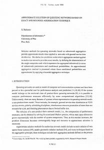
The standard LADM which provides the series solutions given by (7) and the nonlinear terms is decomposed as in (8). In this problem the nonlinear term is N y = y 3 , henceforth using (9) the Adomian polynomials are given by: A0 = y03 A1 = 3y02 y1 A2 = 3y02 y2 + 3y0 y12 A3 = 3y02 y3 + 6y0 y1 y2 + y13 Using the above modified technique, we expand g(x) in the terms of Bernstein polynomials of order 10, g(x) ≈ −0.2461796x10 −1.8849352x9 −5.3246642x8 −6.9170682x7 −4.0861802x6 + 0.5894802x5 + 9.3947682x4 + 32.0678222x3 + 64.3915632x2 + 66.3644302x + 24 (30) In Figure 1. the numerical approximate solution obtained from presented technique is compared with exact solution that exhibits the effectiveness of method. Example 5.2. Consider the nonlinear boundary value problem [12] y ′′ − y 3 = − sin x(1 + sin2 x)

(31)

where y(0) = 0, y(π) = 0 with exact solution y(x) = sin x. Now using the above modified technique, we expand g(x) in the terms of Bernstein polynomials of order 5, g(x) ≈ 0.000788114x5 + 0.136755981x4 − 0.1877757x3 − 0.354509063x2 − 1.032553553x (32)

831

APPROXIMATE SOLUTION OF BOUNDARY VALUE PROBLEM...

3 Exact Solution Presented Method Solution 2.5

y(x)

2

1.5

1

0.5

0 0

0.1

0.2

0.3

0.4

0.5 x

0.6

0.7

0.8

0.9

1

Figure 1: Comparison of Approximate solution with Exact solution

Figure 2. shows that expanding the source term in the Bernstein polynomials, the solution is very much close to the exact solution which proves that our method is well suited to this problem.

6. Discussion Bernstein polynomials are exclusively used to modify the standard Laplace decomposition method. The proposed new technique is analyzed and applied to the nonlinear singular and nonsingular boundary value problems. The results shown in the figures exclude that the numerical approximations are in good agreement with the exact one. The convergence analysis exhibits the applicability of technique.

References [1] M. El-Gamel, Sinc-Galerkin method for solving nonlinear boundary value problems, Computers and Mathematics with Applications, 48 (2004), 1285-1298. [2] D. J. Evans and K. R. Raslan, The Adomian decomposition method for solving delay

832

D. Rani, V. Mishra

0.9

Exact Solution Presented Method Solution

0.8 0.7 0.6

y(x)

0.5 0.4 0.3 0.2 0.1 0 0

0.1

0.2

0.3

0.4

0.5 x

0.6

0.7

0.8

0.9

1

Figure 2: Comparison of Approximate solution with Exact solution

differential equation, International Journal of Computer Mathematics, 82 (2005), 49-54, doi: 10.1080/00207160412331286815. [3] R. T. Farouki, The Bernstein polynomial basis: A centennial retrospective, Computer Aided Geometric Design, 29 (2012), 379-419, doi: 10.1016/j.cagd.2012.03.001. [4] M. M. Hosseini, Adomian decomposition method for solution of nonlinear differential algebraic equations, Applied Mathematics and Computation, 181 (2006), 1737-1744, doi: 10.1016/j.amc.2006.03.027. [5] S. A. Khuri, A Laplace decomposition algorithm applied to a class of nonlinear differential equation, Journal of Applied Mathematics, 1 (2001), 141-155, doi: 10.1155/S1110757X01000183. [6] W. Kim and C. Chun, A modified Adomian decomposition method for solving higherorder singular boundary value problems, Verlag der Zeitschrift fur Naturforschung, 65a (2010), 1093-1100, doi: 10.1515/zna-2010-1213. [7] A. Kumar and R. D. Pankaj, Laplace decomposition method to study solitary wave solutions of coupled nonlinear partial differential equation, ISRN Computational Mathematics, 2012 (2012), 1-5, doi: 10.5402/2012/423469. [8] Y. Liu, Adomian decomposition method with orthogonal polynomials: Legendre polynomial, Mathematical and Computer Modelling, 49 (2009), 1268-1273, doi: 10.1016/j.mcm.2008.06.020. [9] F. Mirzaee and A. A. Hoseini, Numerical solution of nonlinear volterra fredholm integral equations using hybrid block pulse functions and taylor series, Alexandria Engineering Journal, 52, (2013), 551-555, doi: 10.1016/j.aej.2013.02.004.

APPROXIMATE SOLUTION OF BOUNDARY VALUE PROBLEM...

833

[10] H. K. Mishra, He-Laplace method for the solution of two-point boundary value problems, American Journal of Mathematical Analysis, 2 (2014), 45-49. [11] M. A. Mohamed and M. S. Torky, Numerical solution of nonlinear system of partial differential equations by the Laplace decomposition method and the pade approximation, American Journal of Computational Mathematics, 3 (2013), 175-184, doi: 10.4236/ajcm.2013.33026. [12] A. Mohsena and M. El-Gamelb, On the Galerkin and collocation methods for two-point boundary value problems using sinc bases, Computers and Mathematics with Applications, 56 (2008), 930-941, doi: 10.1016/j.camwa.2008.01.023. [13] W. Quain, M. D. Riedel and I. Rosenberg, Uniform approximation and bernstein polynomial with coefficients in the unit interval, European Journal of Combinatorics, 32 (2011), 448-463. [14] K. Sayevand, M. Fardi, E. Moradi and F. H. Boroujeni, Convergence analysis of homotopy perturbation method for Volterra integro-differntial equations of fractional order, Alexandria Engineering Journal, 52 (2013), 807-812. [15] A. M. Wazwaz, The combined Laplace transform-Adomian demcomposition method for handling nonlinear volterra integro-differential equations, Applied Mathematics and Computation, 216 (2010), 1304-1309. [16] S. Widatalla and M. Z. Liu, New iterative method based on Laplace decomposition algorithm, Journal of Applied Mathematics, 2013 (2013), 1-7, doi: 10.1155/2013/286529. [17] C. Yang and J. Hou, An approximate solution of nonlinear fractional differential equation by Laplace transform and Adomian polynomials, Journal of Information and Computational Science, 10 (2013), 213-222. [18] F. K. Yin, W. Y. Han and J. Q. Song, Modified Laplace decomposition method for Lane-Emden type differential equations, International Journal of Applied Physics and Mathematics, 3 (2013), 98-102, doi: 10.7763/IJAPM.2013.V3.184. [19] J. B. Yindoula, P. Youssouf, G. Bissanga, F. Bassono and B. Some, Application of the Adomian decomposition method and Laplace transform method to solving the convection diffusion-dissipation equation, International Journal of Applied Mathematical Research, 3 (2014), 30-35, doi: 10.14419/ijamr.v3i1.1596. [20] S. A. Yousefi and M. Behroozifar, Operational matrices of Bernstein polynomials and their applications, International Journal of Systems Science, 41 (2010), 709-716, doi: 10.1080/00207720903154783. [21] S. Zuhra, S. Islam, M. Idress, R. Nawaz, I. A. Shah and H. Ullah, Solving singular boundary value problems by optimal homotopy asymptotic method, International Journal of Differential Equations, 2014 (2014), 1-10, doi: 10.1155/2014/287480.

834