Nov 6, 1981 - jobs and simultaneous resource possession to networks with ... taneous possession of more than ... the model may ignore the others. Otherwise ...
Charles H. Sauer
Approximate Solution of Queueing Networks with Simultaneous Resource Possession Queueing networksareimportant as Performance models of computer andcommunication systemsbecause the performance of these systems isusually principally affected by contention for resources.Exact numerical solution of a queueing network is usually only feasible ifthenetwork has a product formsolution in the sense of Jackson. Animportant network characteristic which apparently precludes a product form solution is simultaneous resource possession, e.g., a j o b holds memory and processor simultaneously. This paper extends previous methods for approximate numerical jobs and simultaneous resource possessionto networkswith solution of queueing networkswithhomogeneous heterogeneous jobs and simultaneous resource possession.
1. Introduction A major objective of computing systems (including computer communication systems) development in the last two decades has been to promotesharing of system resources. Sharing of resources necessarily leads to contention, i.e., queueing, for resources. Contentionand queueingfor resources are typicallyquite difficult to quantify when estimating system performance. A major research topic in computing systems performance in the last two decades has been solution and application of queueing models. These models are usually networks of queues because of the interactions of system resources. For general discussion of queueing network models of computing systems, see Sauer and Chandy[ 11 and recent special issues of Computing Surveys [2] and Computer Dl.
Much ofthe attention in queueing networkresearch has been given to models with a product formsolution in the sense that
P(S1,* . ) , S e,
=
PI(S,)*
* *
G
P&f(S&$ t
where P(Sl, SM) is the probability of a network state in a network with M queues, Pm(Sm),m = 1, . . M , is a factor corresponding to the probability of the state of queue m , and G is a normalizing constant. The existence of a productformsolution for a modelmakesnumerical a,
a ,
solution feasible wherea large number of queues andlor jobs would otherwise make numerical solution infeasible. Since the original work ofJackson [4], it has been shown that the product form solution exists for networks with heterogeneous jobs, several important scheduling disciplines,and state-dependent behavior [5-71. Efficient computational algorithms have been developedfor these networks [8-113. However, there are a number of system characteristics which apparently preclude a product formsolution. Among the mostimportant of these issimultaneous resource possession, i.e., a job’s activities require simultaneouspossession ofmorethan one resource, e.g., memory and processor. If there is significant contention for only one of the simultaneously held resources, then the modelmay ignore the others. Otherwise, one must usually settle for an approximatenumericalsolution [12, 131 or simulation. paper This focuses on approximate numerical solution of models with simultaneousresource possession in cases such as the one depicted in Fig. 1. In this case a job holding memory may simultaneously also hold the CPU or simultaneously also hold a disk. Further, requests for and releases of simultaneously held resources are nested, Le., memoryis requested before the CPU is requested
Copyright 1981 by International Business Machines Corporation. Copying is permitted without payment of royalty provided that (1) each reproduction is done without alteration and (2) the Journal reference and IBM copyright notice are included on the first page.
894
i
The title and abstract may be used without further permission in computer-based and other information-servicesystems. Permission to republish other excerpts should be obtainedfrom the Editor.
CHARLES H.SAUER
IBM 1. RES. DEVELOP.
0
VOL. 25
0
NO. 6
NOVEMBER 1981
rL“-
and released after a disk is released. With such nesting pMae;:s , one can transform the original network into one of the Disk I form of Fig. 2. A solution of the transformed network can then be interpreted as an approximate solution of the Terminals original network. The approximate solution will usually bemuch less expensive thansimulation. It is quite difficult to estimate the error in the approximate solution, but empirical studies suggest the error is acceptable in 1 J many situations. Some of the influential works using this approach for modelssimilar to this one are those of Figure 1 Queueing networkmodel of interactive computer Brandwajn [14], Brown [15, 161, Courtois [17, 181, and system. Keller [19]. This general approach can be appliedto other resources and to more than two simultaneouslyheld resources. For an introduction to previous work using this approach, see the survey papers by Chandyand Sauer [12, 131. Two other approaches to solution of this , -- - - - - I problem are those of Bard [20] and Jacobson and LaR0 I I c= zowska [21]. Terminals Composite 0
0
-
FZ t;
Except for the work ofBard[201 andNewsomand Ward 1221, previous assumed efforts have that jobs were homogeneous. Our interest here is extending the above general approach to networks with heterogeneous jobs. Though Bard’s approach applies to fairly general cases with heterogeneousjobs, we find it less accurate than our approach for many cases; see the Appendix for further discussion.NewsomandWard attempted to extend Brown’swork[15, 161 to heterogeneous jobs. Though they wereable to extend the relevant equations, the result was computationally impractical, as they discussed. Further, only two test cases were considered in their paper. In Section 2 we consider the model of Fig. 1 without memory contention in order to develop previous results onflow-equivalence, the basis of this work. In Section 3 we consider the model of Fig. 1 with heterogeneous jobs where separate memory is dedicated to each type of job. In Section 4 we consider the case where the different types of jobs share memory. Empirical results demonstrate the effectiveness of the methods used. 2. Flow-equivalence
A principal objective in the transformation of the network of Fig. 1 to the network of Fig. 2 is to obtain flowequivalence, i.e., the flow of jobs through the composite queue of Fig. 2, given a specific populationof jobs in that queue, is equivalent to the flowof jobs through the corresponding subnetwork of Fig.1,given the same population of jobs in the subnetwork. This can be approached either by using “Norton’s Theorem” for queueing networks, analogous to Norton’s Theorem for electrical circuits [23], or by using concepts of weak-coupling of subnetworks [17].We use the Norton’sTheorem approach.
IBM J. RES. DEVELOP.
VOL. 25
NO. 6 0 NOVEMBER 1981
0
r-l~
~
I I
Figure 2 Computersystemmodel replaced by composite queue.
with CPU and I/O disks
Disk
Figure 3 CPU anddisksubnetwork.
Let us assume that there are two types of jobs, numbered 1 and 2. Extension to more than two types of jobs is conceptually trivial. (Extension to more than a few job types may be computationally prohibitive, as with other queueing network problems.) Let the number of type k jobs be Nk,k = 1, 2. The Norton’s Theorem approach to this problem is straightforward. We would consider the network of Fig. 1 with the terminals queue “shorted,” e.g., with service time set to zero. Our intermediate objective is to obtain the throughput through the “short.” To obtain the desired throughput, we need only solve the network of Fig. 3 to obtain the throughput through the outer loop. Let
895
CHARLES H.SAUER
1
Terminals
be obtained by Little’s Rule. Utilizations can beobtained either from throughputs or marginal queue length distributions, dependingon the characteristics of the individual queues. For more discussion of individual queue measures see Sauerand Chandy [l, Section 6.3.31. This entire process is exact provided thatthe original network satisfies product form.
Composite
Figure 4 Computersystemmodelwithmemory,CPU,and disk replaced by composite queue.
Rk(n,, n,) be the throughput of type k jobs through the outer loop of Fig. 3 given n1type 1 jobs and n, type 2 jobs in thatnetwork, k = 1 , 2 , n , = 0, . -,N , , n2 = 0, N,. Then let the composite queue of Fig. 2 have service rate pk(n,,n,) = Rk(n,, n,) for type k jobs when there are n, type 1 jobs and n2 type 2 jobs in the composite queue. Both types of jobs are in service simultaneously when both types of jobs are presentin the queue. e,
Since we have assumed for the moment that there is no memory contention, the network of Fig. 2 is equivalent to the network of Fig. 4. The network of Fig. 4 satisfies productform if the original networksatisfiesproduct form (assuming no memory contention). Several computational algorithms for product form networks apply to the network of Fig. 4 if it satisfies product form [ll]. However, composite queues with general functionsof the form pk(n,,n,), such as the oneswe obtain below, do not necessarily satisfy product form conditions. Assuming that the network of Fig. 1 satisfies product form (assuming no memory contention), then the throughputs through the terminals are the same in the network of Fig. 1 and the networks with the composite queue (with nonzero service time at the terminals). Further, the performance measures for the CPU and disk queues can be obtained from the solutions of the networks of Fig. 2 and Fig. 3. Throughputs are immediately available by flow arguments. Marginal queue length distributions and moments of queue length can be obtained as weighted sums where the weights are thevalues of the composite queue marginal queue length distribution. For example, mean queue length of type k jobs at the CPU can be obtained as
where P(n,, n,) is the marginal probability of n , type 1 jobs and n, type 2 jobs in the composite queue and L:,cpU(n,, n,) is the mean queue length of type k jobs at the CPU in the network of Fig. 3, given n , type 1jobs and n2 type 2 jobs in that network. Mean queueing times can
3. Dedicated resources In this sectionweconsider thecasethat the outer resource in the nesting (memory in our example) is managed so that different types of jobs have different dedicated units of the resource. The inner resource in the nesting (CPU or disk in our example) is sharedamong all jobtypes. This case ismoretractablethanthe fully shared resource case of Section 4. Let us assume thatmemory is organized in T partitions and that each job requires exactly one partition. In this section we assume that there are T , partitions dedicated to type 1 jobs and T2 partitions dedicated to type 2 jobs (TI + T, = T ) . We assume in this section that, within a job type, memory is scheduled First-Come-First-Served (FCFS), independent of the other type. The discussion in this section extends directly to the more general memory organizations considered by Brownfor homogeneous jobs [161.
Now we return to thecase of interest, i.e., where there is memory contention. Essentially the above process is followed, but there are two new issues to be considered. First, the solution of the network of Fig. 2 no longer gives exact values for the measures for the network of Fig. 1. This is easily demonstrated by example, but it is quite difficult to characterize the amount of error. The second issue is the solution of the network of Fig. 2. We can immediately transform the networkof Fig. 2 to that of Fig. 4 by recognizing that therewill never be more than Tk type k jobs in the composite queue, k = 1, 2 . Thus, we can let the service rate function for the composite queue be
&&, n2) = Rk(min (TI, nl), min V,, n2N,
(1)
wherek=1,2,n,=0;..,N,,n,=0;**,N2.
A composite queue with this rate function does not necessarily satisfy product form. However, the network of Fig. 4 with this rate functionis easily solved by considering the underlying Markov process. Many numerical approachesapplyreadily tosuch a Markov process. Gauss-Seidel iteration and the related methods considered by Stewart [24] are obvious possibilities. Brandwajn’s recent iterative method could be used [25].
IBM J. RES. DEVELOP.
0
VOL. 25
NO. 6
0
NOVEMBER 1981
We,somewhatarbitrarily, chooseto applyHerzog’s method [26] to this problem; see [27] for details. Since it is diacult to characterize the error introduced by the replacement of the subnetwork of Fig. 1 by the composite queue, it is necessary to empirically evaluate the approximate method. Ideally, one would run experiments for a wide parameterspace of models. Inour experiments we fixed several parameters (see Table 1) and varied N , , N 2 , Tand I , T2.Three pairs of values were used for ( N , , N J ,(20, 2), (30, 3), and (40, 4). T , and T2 were chosen as follows. For a given ( N , , N 2 )pair, the network was evaluated assuming no memory contention. (All of thenetworks evaluatedsatisfy product form except for memorycontention.)One ( T I , T2) pairwas chosen so that Tk, k = 1, 2, was approximately equal to the mean memory queue length of type k jobs, Lk,Memory, in the network without memory contention.Inother words, Tk Nk - Lk,Teminals9 where Lk,Terminals isthe mean type k queue length at the terminals in the network without memory contention. Thisshould result in moder- 2 ate memory contention. The other twopairs were chosen to have T 50% larger, i.e., minimal memory contention, and to have T 50% smaller, i.e., severe memory contention. Table 2 gives the nine parameter combinations. Reference valueswere obtained by simulation using the Research Queueing Package (RESQ)[28, 291. Confidence intervalswereobtained using the regenerative method [30]. A sequential stopping rule [31] was used to obtain a relative width of 5% for the confidence interval for the type-independent mean response time (mean time from memory request tomemory release for all jobs) at a 90% confidence level.Table 2 also gives theCPU time in seconds spent on these simulations on an IBM 370/168. For eachof the nine cases, the CPUtime for approximate solution was less than one-half second on a 168. Since the simulation point estimates are not exact, and a confidence interval does notnecessarilycontain the corresponding true value, it is not clearhow accuracy of the approximation values should be judged. The following criteria are somewhat arbitrary and may be more stringent than required by many applications. Given a performancemeasure v fromthe approximation,let us construct an interval (v - 6, v + 6) such that it is the smallest interval that (partially) overlaps the simulation confidence interval for this measure. If 6 5 0.05 x v, then the approximation valueis considered satisfactory; if 6 5 0.10 X V, then the approximation value is considered in error; andif 6 > 0.10 x v, then the approximation value is considered severely in error. These criteria were applied to the approximation results for all queues (terminals, memory, CPU, anddisks)
IBM J. RES. DEVELOP.
0
VOL. 25
0
NO. 6
0
NOVEMBER 1981
Table 1 Parameters fixed for allexperiments.
Mean think time: type 1-5 seconds, type 2-10 seconds. (exponential distribution, “Infinite Server” discipline) Mean number of CPU-I/O cycles: type 1-10, (geometric distribution)
type 2-20.
Mean CPU service time: type 1-10 ms, type 2-100 ms. (exponential distribution, Processor Sharing discipline) Four identical disks with same parameters for each type: Branching probabilities from CPU to disk: 0.25. Mean disk service time: 35 ms. (exponential distribution, FCFS discipline)
Table 2 Dedicatedmemory parameter combinations. Simulation time
Case
(SI
1 2
4 20 3 20 20 30 30 30 40 40 40
2 2 2 3 3 3 4 4 4
1 7 5 2 14
9 5
1 1 2 1 1 4 3 1
403 525 330 507 594 442 603 984 816
for both type-dependent and type-independent measures of utilization, throughput, mean queue length and mean queueing time. (The memory queueing time is defined as time from request until release.) The approximation results were satisfactory for all nine parameter combinations for all measures except for type-dependent CPU utilization. The type 1 CPU utilization was underestimated andin error forall nine combinations. The type2 CPU utilization was overestimated andin error forall combinations except combination 3, wherethetype 2 CPU utilization was satisfactory. Table 3 givesthe approximation values and simulation confidence intervals for typeindependent CPU utilization ( U ) and mean response times(memoryqueueingtime Q ) and type-dependent mean response times. The achieved accuracy seemsmore than adequate for most applications, and the approximation solutions required roughly three orders of magnitude less computation than the simulations. 4. Shared resources
In thissection we consider thecasethattheouter resource in the nesting(memoryin our example) is managed so that different types of jobs share the same
897
CHARLES H.SAUER
Table 3 Dedicated memory performance measures. Case
1 2 3 4 5 6 7 8 9
0.62 0.60 (0.48, 0.49 0.84 0.80 (0.69, 0.69 0.96 0.95 0.87
________
(0.60, 0.63) (0.59, 0.61) 0.50) (0.83, 0.85) (0.79, 0.81) 0.71) (0.96, 0.97) (0.95, 0.96) (0.87, 0.88)
0.95 1.08 4.79 1.28 1.42 4.23 1.83 2.00 2.69
(0.91, 0.95) 1 . 1(11). 0 6 , (4.64, 4.87) (1.24, 1.30) (1.37, 1.44) (4.09, 4.30) (1.79, 1.87) (1.98, 2.07) (2.65, 2.78)
units of that resource. Thus, all types of jobs share exactly the samesimultaneouslyheld resources. This case is, perhaps, moreimportantthan the dedicated resource case. Unfortunately, the shared resource case also seems more difficult. The difficulty isin transforming thenetwork ofFig. 2 to that ofFig. 4, to avoidthe relatively expensive solution of the network of Fig. 2. The difficulty of this transformation depends on the memory scheduling discipline; for some of the most interesting disciplines an accurate transformation does notseem feasible. For strictly preemptive priority, theappropriate transformation seems, assuming type 1jobs have higher priority, to use pk(nl,n2) = R,(min (T, n,), min ( T - min ( T , n , ) , n,)),
(2)
k = 1, 2. Corresponding to Eq. (l), Eq. (2) gives a simple and intuitively reasonable basis for selecting a specific Rk(il,i2) to use for pk(n,, n,) when n, + n, > T . For other disciplines, suchas FCFS or non-preemptive priority, there seems to beno comparablysimple or intuitively reasonable basis for the transformation. The problem is that the representation of memory and the nested subnetwork by a function of the form p,(n,, n,) discards essential state information. For the FCFS disciplineweinvestigated a number of weightedsumapproaches, e.g., equal weights: min(T,nz)
C Fk(n,, ",)
=
R,(min (T - t , n,), t )
t=T-min(T,n,)
min (T, n,)
n, + n,
L
Ql,Mernory
QMernory
UCPU
+ min (T, n,) + 1 - T
T,
k
= 1,
2,
' (3)
but all approaches attempted resulted in severe underestimates of response times. (Since the methodof Newsom
0.80 0.93 4.83 1.06 1.17 4.10 1S O 1.69 2.33
(0.77, 0.80) (0.90, 0.95) (4.68, 4.93) (1.03, 1.08) (1.13, 1.19) (3.97, 4.17) (1.47, 1.54) (1.67, 1.74) (2.30, 2.42)
QZ.Memory
4.66 5.08 4.09 7.59 9.13 6.44 13.30 12.46 14.47
(4.49, 5.09) (4.71, 5.31) (3.86, 4.31) (6.70, 7.64) (8.42, 9.69) (6.08, 6.95) (12.15, 14.10) (11.98, 13.26) (13.48, 15.15)
and Ward attempts this transformation, we are skeptical of its accuracy until it has been subjected to significant empirical evaluation.) For these reasons, we accepted the expense of solving the networkof Fig. 2. This allows us to simply use p,(n,, n,) = R,(nl, n,). Herzog's method [261 does noteasily extend to the network ofFig. 2. Sincetheunderlying Markov process is not a two-dimensional birth anddeath process, Brandwajn's recent method [25] does not apply. However, Gauss-Seideliteration and the related methods considered by Stewart [241 do apply. We choose to use Gauss-Seidel iteration. Implementation details are given in [27].With non-preemptive prioritythere are no further difficulties.With FCFS there is the problem that the Markov states of the network of Fig. 2 mustinclude information on the ordering ofjobs in the memoryqueue, and thus the number of states is too large for numerical solution to be feasible. For this reason, we introduce another approximation, representing FCFS schedulingby randomscheduling. With randomscheduling,ordering information is not required for a Markov process representation, and numerical solution is feasible. Besides scheduling,there is another issue of interest in the shared resource case which is a minor consideration in the dedicated resource case: The different job types may require different amounts of resource. So let us now consider T to be the number of abstract units of memory available and A,, k = 1, 2, to be the number of units required by each type k job. When different types of jobs havedifferent resource requirements, First-Fit (FF) scheduling is usually more interesting than FCFS. FF is thesame as FCFS except that a satisfiable request is satisfied even when a job ahead in the queue must wait because its request is greater than the number of units currently available. This issue has little impact on the
IBM J. RES. DEVELOP. 0 VOL. 25
0
NO. 6
0
NOVEMBER 1981
difficulty of numerical solution of the network of Fig. 2. The more general memory organizations considered by Brown are easily incorporated in the iterative solution of the network of Fig. 2 [27].
Table 4 a ) Shared memory parameter combinations and error summary for First Come First Served memory scheduling and homogeneous memory requirements (1 unit). ~~~~~
Case N , N2
Ind. errors
Run time
Dep. errors ______
Tables 4 and 5 summarize the cases considered in empirical evaluation of these methods. There are six groups of nine cases, with one case in each of those groups corresponding to one of the casesof Table 2. The first three groups have the same memoryrequirement for each job type. In the second three groups the second job type requires four times as much memory as the first. The first group has FCFS scheduling. The second and fifth groups have non-preemptive priority schedulingwith type 1 jobs having higher priority. The third and sixth groups have non-preemptive priority schedulingwith type 2 jobs having higher priority. The fourth group has FF scheduling. In Table 4 the column headed “App.” gives the number of CPU seconds required for the approximate solution on a 370/168. Similarly, the column headed “Sim.” gives the simulation CPU time. The four columns under “Ind. Errors” give the numbers of typeindependent errors and severe errors for utilization (V), throughput (R),mean queue length (L),and mean queueing time (Q). (The maximum numberof errors for a given measure isseven, one per queue.) Similarly the remaining four columns givethe numbers of type-dependent errors. (The maximum number of errors for a given measure is fourteen, two per queue.) Table 5 has the same format as Table 3. It gives the approximation values and simulation confidence intervals for CPUutilizationandmean response times. Measures with errors and severe errors are preceded by “e” and “s,” respectively. Generally speaking, the accuracy is good, though not as uniformly good as for the dedicated memory cases. The priority cases seem as free of errors as the dedicated memory cases, but case 14 (FCFS) and cases 42 and 45 (FF) have many errors. Even for these three cases the accuracy would likely be sufficient for many applications. The CPU time comparisons, though still quite favorable, are not as good because of the relatively “brute-force” iterative methods used for the solution of the network of Fig. 2.
U R L Q U R L Q
T App. Sim. 10 11 12 13 14 15 16 17 18
20 20
20 30 30 30 40 40 40
2 2 2 3 3 3 4 4 4
6 4 2 9 6 3 18 12 6
1 1
2
I 8 9 20 23 28
379 733 971 422 876 1394 669 1185 1343
0 0 0 1 1 0 0 0 0
0 0 0 0 0 0 0 0 0
0 0 0 0 5 0 0 0 0
0 0 0 0 2 0 0 0 0
2 0 0 0 1 0 0 0 0 0 0 0 4 0 0 0 3 0 5 3 0 0 0 0 2 0 0 0 1 0 0 0 0 0 0 0
Table 4(b) Shared memory parameter combinations anderror summary for priority memory scheduling (type 1 has higher priority) and homogeneous memory requirements (1 unit). ~~~
Case N ,2
Run time
~~
Ind. errors
Dep. errors
T App. Sim. U R L Q U R L Q 19 20 21 22 23 24 25 26 21
20 20 20 30 30 30 40 40 40
2 2 2 3 3 3 4 4 4
6 4 2 9 6 3 18 12 6
1 1 2 7 7 8 18 21 26
319 604 819 594 1076 834 806 178 680
0 0 0 0 0 0 0 0 0
0 0 0 2 0 0 0 0 0 0 2 0 0 0 0 0 0 0 0 0 0 0 0 0 2 0 0 0 0 0 0 1 0 0 0 0 0 0 1 0 1 1 0 0 0 2 0 0 0 0 0 0 1 0 0 0 0 0 0 0 0 0 0
Table 4(c) Shared memory parameter combinations and error summary for priority memory scheduling (type 2 has higher priority) and homogeneous memory requirements (1 unit). Case
N ,2
Run time
Ind. errors
Dep. errors
T App. Sim. U R L Q U R L Q
5. Summary We have shown how the “Norton’sTheorem” approach to approximate solution of queueing networks with simultaneous resource possession can be extended to networks with heterogeneous jobs. We have empirically demonstrated the accuracy of the approach and shown that the approximation is typically two orders of magnitude less expensive than simulation.Both the accuracy and ex-
IBM J . RES. DEVELOP. a VOL. 25 a NO. 6
0
NOVEMBER 1981
28 29 30 31 32 33 34 35 36
2 0 2 0 2 0 3 0 3 0 3 0 40 40 40
2 2 2 3 3 3 417 4 4
6 4 2 9 6 3 18 12 6
1 1 1 6 7 8
19 23
439 708 1394 634 1375 1507 613 1087 1623
0 0 0 0 0 0 0 0 0
0 0 0 0 0 0 0 0 0
0 0 0 0 0 0 0 0 0
0 0 0 0 0 0 0 0 0
1 2 0 2 2 0 2 1 0
0 0 0 0 0 0 0 0 0
0 0 0 0 0 0 0 0 0
0 0 0 0 0 0 0 0 0
899
CHARLES H. SAUER
Table 4(d) Shared memory parameter combinations and error summary for First Fit memory scheduling and heterogeneous memory requirements (type 1jobs require 1 memory unit, type 2 jobs require 4 memory units).
penseshouldbe acceptable inmanyapplications,but some applications will require better accuracy or lower expense.
Case N ,
Though the focus has been on the memory contention model of Fig. 1, our discussion applies directly to other examples of simultaneous resource possessionand to more than two simultaneously held resources, as in the homogeneous job case. Similarly,though we have assumed the network satisfies product form except for the simultaneous resource possession, the approach applies readily to non-product form networks which are amenable to flow-equivalence approximate solution.
37 38 39 40 41 42 43
44 45
20 20 20 30 30 30 40 40 40
Run time
2 2
2 3 3 3 4 4 4
Ind. errors
Dep. errors
T App. Sim.
U R L Q U R L
Q
11 7 4 14 9
0 0 0 0 0 0 0 0 0 0 0 0 0 0 0 0 0 5 0 0 0 0 0 1 0 0 0
0 0 0 0 0 2 0 1 9
5
27 18 9
3 4 4 23 25 21 58
84 87
401 493 2048 1049 1518 3302 524 1731 2271
0 0 0 0 0 1 0 1 3
2 2 2 2 2 1 0 2 0 3
0 0 0 0 0 7 0 0 0
0 0 0 0 0 1 3 0 1 5
Table 4(e) Shared memory parameter combinations and error summary for priority memory scheduling (type 1 has higher priority) and heterogeneous memory requirements (type 1 jobs require 1 memory unit, type 2 jobs require 4 memory units). Case N , N2
Run time
Ind. errors
Dep. errors
T App. Sim. U R L Q U R L 46 41 20 48 49 50 51 52 53 54
2 0 2 1 1 2 0 2 7 2 4 30 3 14 3 0 3 9 3 0 3 5 40 4 27 40 4 18 4 0 4 9
1 4 0 1 0 0 0 0 2 0 0 1 4 6 7 0 0 0 0 2 0 0 1 1 5 3 3 0 0 0 0 2 0 0 7 8 5 4 0 0 0 0 2 0 0 8 1 3 0 0 0 0 0 0 2 0 0 5 1 0 8 1 0 0 0 0 2 0 0 19 6 2 4 0 0 0 0 2 0 0 23 7260 0 0 0 2 0 0 17 4 2 6 0 0 0 0 2 0 0
Q 0 0 0 0 0 0 0 0 0
Table 4(f) Shared memory parameter combinations and error summary for priority memory scheduling (type 2 has higher priority) and heterogeneous memory requirements (type 1 jobs require 1 memory unit, type 2 jobs require 4 memory units). Run time
Case N N ,,
T App. Sim. 55 56 57 58 59
900
60 61 62 63
CHARLES H. SAUER
20 20 20 30 30 30 40 40 40
2 2 2 3 3 3 4 4 4
11 7 4 14 9 5 27 18 9
3 4
3 21 22 5 53 74 66
Ind. errors
U R L Q U R
0 0 0 0 0 0 409 0 2460 0 2797 0 437 2260 2519 1326 2956 989
Dep. errors
0 0 0 0 0 0 0 0 0
0 0 0 0 0 0 0 0 0
0 0 0 0 0 0 0 0 0
2 2 2 2 2 2 2 2 2
0 0 0 0 0 0 0 0 0
L Q 0 0 0 0 0 0 0 0 0
0 0 0 0 0 0 0 0 0
Appendix: Bard’s method Bard’s method for handling memorycontention provides a verysimple iterative approach [20]. The principal advantage of the approach is that it is very inexpensive. The method is generally less accurate than the methods we have described. A fundamental assumption of the approach is that, if there is sufficient memoryon the average for a given type of job, then that job never waits for memory. Thetypes of jobs are partitioned into “trivial” and “non-trivial” types; it isassumed that trivial jobs neverwaitfor memory. Our discussion here assumes all jobs are nontrivial jobs.
Let there be K job types. The following discussion assumes A, = 1, k = 1, * -,K . It is simple to extend the discussion to avoid that assumption. From Little’s Rule one can reasonably say that the mean number of type k jobs holding memory is
where H , is the mean time type k jobs spend holding memoryand W, is the mean timetype k jobs spend waiting for memory. Thus K
1*kQ k=l
Hk ,,Terminals + wk
5
-k
T.
(A21
Hk
If (A2) results in a strict inequality, then it is assumed that there is no memory contention. This can clearly resultin noticeable errors if the left-hand side of (A2) is nearly as large as the right-hand side.If (A2) results in an equality, then one must solve that equation for W,,k = 1, * . K . This solution depends on memory scheduling. Bard considers two cases, FCFS and “Fair-Share,” a discipline used inthe IBM VMl370 operating system. We ignore the Fair-Share discipline. Theapproach does not apply to FF a,
IBM J. RES. DEVELOP.
VOL. 25
NO. 6
NOVEMBER 1981
Table 5(a) Shared memory performance measures for First Come First Served memory scheduling and homogeneous memory requirements. Case
UCPU Q1,Memory
QMemory
Q2,Mulemory
~
0.62 0.61
10 11
54 84
12 13 14 15 16 17 18
96 95
'
'
(0.60, 0.63) (0.60, 0.62) (0.53, 0.54) (0.82, 0.84) (0.83, 0.85) (0.69, 0.71) (0.95, 0.96) (0.95, 0.96) (0.90, 0.90)
0.82 0.71 0.90
0.90 1.08 2.57 1.29 e1.62 3.75 1.82 1.99 3.49
(0.87, 0.91) (1.05, 1.10) (2.46, 2.59) (1.20,1.26) (1.40,1.47) (3.60, 3.78) (1.78,1.87) (1.94, 2.03) (3.44, 3.61)
0.75 0.93 2.45 I (1 .08 S I .42 3.59 1S O 1.71) (1.64, 1.68 3.24
(4.34,4.73 (0.73, 0.76) 4.93) 4.60 (0.91, 0.95) (4.85,4.98 (2.35, 2.47) 5.12) .oo, 1.04) 7.48 (1.20, 1.26) 7.47) (6.87,6.89 6.87 (3.44, 3.62) (1.47, 1.54) (12.41, 14.00) 13.40 12.74) (11.63, 12.49 9.33 (3.19, 3.35)
Case
Ql,Memory UCPU
1
(6.79, 7.01) (9.23, 9.81)
QMemory
19 0.64)(0.60, 0.90 5.02)(4.39, (0.88, 4.740.93) 0.77)(0.74, 0.75 20 (0.60, 0.62) 1.05 (1.03, 1.08) 0.914.78 0.93)(0.89, 21 0.50 1.95)(1.86, (0.49,1.91 0.50) 2.22)(2.11,2.16 0.84 1.07 22 1.30)(1.24, 1.28 0.84)(0.82, (1.04, 1.09) 0.82 23 1.53 0.82)(0.81, (1.50, 1.31 1.58) 7.92)(7.27,(1.29, 7.63 1.35) 0.59 24 (0.59, 0.60) 27.30) (24.07, e22.49 2.77 2.43)(2.32, (2.78, 2.32 2.91) 25 1 S14.15) O(12.64, 13.41 1.53) (1.47, 0.96 1.86) (1.78, (0.95, 1.820.96) 3 2.00)(1.91, 1.95 26 0.96)(0.95, 0.95 27 2.70)(2.58, 0.822.67 0.82)(0.81, 2.25 2.13) (17.84, (2.19, 19.372.28)
2
7.92) (6.95,
Table5(b) Shared memory performance measures for priority memory scheduling (type 1 has higher priority) and homogeneous memory requirements.
,Memory
2
(4.46, 4.88)
0.62 0.61
9.45 (6.78, 7.53
(4.39, 4.81) (9.35, 10.23) 7.61)
Table 5(c) Shared memory performance measures for priority memory scheduling (type 2 has higher priority) and homogeneous memory requirements. Case __
28 29 30 31 32 33 34 35 36
0.61 0.55 0.84
0.73 0.96 0.95
UCPU
Q, ,Memory
QMemory
(0.62, 0.65) (0.60, 0.62) (0.54, 0.55) (0.84, 0.86) (0.81, 0.82) (0.73, 0.74) (0.95, 0.96) (0.95, 0.96) (0.91, 0.92)
0.90 1.09 2.79 1.29 1.66 4.25 1.82 2.01 3.83
(0.90, 0.94) (1.04, 1.09) (2.68, 2.81) (1.27, 1.34) (1.59, 1.67) (4.22, 4.44) (1.75,1.83) (1.94, 2.04) (3.78, 3.97)
0.78) (0.75, 0.75 0.95 2.76) (2.62, 2.73 (1.06, 1.08 1.48) (1.41, 1.47 4.40) (4.19, 4.22 IS O 1.72) (1.64, 1.69 3.77) (3.58, 3.64
QZ,Memory
4.72 (0.91, 0.95)4.53)(4.16,4.51 3.75)(3.60,3.78 8.1 (7.24, 7.46 1.11) 6.65 4.98)(4.74,4.77 (1.45, 1.51) 13.78) (12.06, 13.40 12.39 8.18)(7.72,7.84
(4.56, 5.11) 1)
(6.22, 6.67) (11.68, 12.97)
Table 5(d) Shared memory performance measures for First Come First Served memory scheduling and heterogeneous memory requirements. Case
37 38 39 40 41 42 43 44 45
UCPU
0.62 0.63) (0.61, 0.60 0.52 0.84) (0.83, 0.84 0.81) (0.80, 0.80 0.67) (0.66, 0.66 0.96 0.96) (0.95, 0.95 0.86) (0.78, 0.85
IBM J . RES. DEVELOP.
QMemory
(0.60, 0.63)
0.53) (0.52,
(0.96, 0.97)
VOL. 25
NO. 6
0.91 1.02 2.09) (1.99, 1.96 1.44) (1.37, 1.34 I .69 s.2.48 1.88) (1.79, 1.83 e2.05 2.71
NOVEMBER 1981
(0.86, 0.90) (0.97, 1.01) (1.59, 1.67) (2.75, 2.84) (2.21, 2.32) (2.53, 2.61)
Q1,Memory
0.76 0.84) (0.80, 0.86 1.88) (1.78, 1.74 1.23) (1.17, 1.13 1.47 2.53) (2.45, s2.12 1.51 s1.74 2.33
(0.72, 0.75)
(1.37, 1 . 4 4 ) 1.54) (1.48, (1.92, 2.01) (2.18, 2.26)
Q2,Memory
4.72 5.18 7.52 7.36 7.64 s15.34 13.34 12.28 e16.29
(4.29, 4.82) (5.10, 5.71) (6.95, 7.28) (6.81, 7.32) (7.51, 8.07) (11.57,12.02) (12.09,14.13) (11.13,11.87) (14.13,15.08)
CHARLES
90'1
n. SAUER
Table 5(e) Shared memory performance measures for priority memory scheduling (type 1 has higher priority) and heterogeneous memory requirements. Case
0.62 0.61 0.52
Ql,Memory UCPU
46 47 48 49
0.84 0.80
50
0.65 0.85
51 52 53 54
0.96 0.95
__
(0.60, 0.63) (0.60, 0.62) (0.52, 0.53) (0.82, 0.84) (0.80, 0.81) (0.65, 0.66) (0.95, O.%) (0.95, 0.96) (0.83, 0.85)
0.91 0.97 1.85 I .32 1.55 2.19 1.83 1.97 2.23
Q2,Mernory
QMemory
(0.86, 0.90) (0.94, 0.99) (1.81,1.90) (1.27, 1.33) (1.52,1.60) (2.14, 2.25) (1.75, 1.84) (1.89,1.98) (2.14, 2.25)
0.75) (0.72, 0.76 0.83) (0.79, 0.81 I .62 1.11 1.32 1.85) (1.76, 1.80 1.51 (1.59, I .65 1.83) (1.74, 1.82
(1.58, (1.06,
1.36) (1.30, (1.46,
4.82)(4.29,4.72 5.47)(4.85,5.28 1.67)8.47)(7.99,8.22 1.11)7.54)(6.87,7.43 8.61)(7.86,8.21 19.44) (17.69, 18.44 13.32) (11.57, 13.35 1.52) 13.18) (11.83, 12.77 1.66) 21.77) (19.26, 2.96
Table 5(f) Shared memory performance measures for priority memory scheduling (type 2 has higher priority) and heterogeneous memory requirements. Case
QI,Memory UCPU
-
55 0.62 (0.60, 0.91 0.62) 0.60) (0.59,0.60 56 2.980.54) (0.53,0.54 57 0.83 (0.83, 1.41 0.84) 58 (0.80,0.81 0.81) 59 (0.65,0.65 0.66) 60 61 0.97) 1.83 (0.95,0.96 62 0.952.30 0.95)(0.95, 63 5.290.88) (0.87,0.88
QMemory ~
(0.87, 0.92) 1.18 1.31) (1.25, (2.75, 2.92 2.88) 1.41) (1.34, 2.08 2.26) (2.14, 2.24 1.84) (2.13, (1.75, 1.80 2.24) 2.19 (1.81, 1.90) 2.01 (2.20, 2.32) 5.26) (5.02, 5.23 5.33) (5.08,
Q2,Memory
___-_____
(0.74, 0.76
1.32
1.21 1.56) (1.49, 1.51
0.77) 4.70 (4.52,4.59 (1.11, 1.17) 4.74) 4.06 (2.67, 2.81) 7.29) (6.78,7.08 1.20) (1.14, 5.66 (1.99, 2.10) 18.44 13.32 10.93 (I2.02) .92, 6.26
(4.27, 4.77)
(5.55, 5.77) (17.58, 19.36) 14.39) (12.51, (10.61, 1 I .20) (6.17, 6.34)
e4.07 e4.07 s5.74 s5.33 s5.33 7.10 e11.51 11.51 e8.47
(4.34, 4.93) (4.46, 4.88) (4.85, 5.12) (6.95, 7.92) (6.87, 7.47) (6.69, 7.01) (12.41,14.00) (11.63,12.74) (9.23, 9.81)
(4.10, 4.25)
Table A1 Shared memory performance measures (Bard's method). Q2,Memory
Case
Ql,Memory UCPU
QMemory
__"
10 11 12 13 14 15 16 17 18
0.64 0.64 0.51 e0.90 (0.82, 0.84) eO.90 (0.69, 0.71) 0.70
(0.60, 0.63) (0.60, 0.62) (0.53, 0.54)
1.00
(0.95, 0.96) (0.95, O.%) 0.90)
1.00 (0.90, 0.94
(0.83, 0.85)
e0.80 s0.80 e2.87 s1.01 s1.01 3.87 e1.63 S I .63 e3.18
(0.87, 0.91) (1.05,1.10) (2.46, 2.59) (1.20,1.26) (1.40,1.47) (3.60, 3.78) (1.78, 1.87) (1.94, 2.03) (3.44, 3.61)
or priority disciplines of the sort we have considered. With FCFS, Bard assumes that all job types have the same mean wait for memory, W. The iteration proceeds by assuming values forHk, k = . K. When (A2)results in an equality, it becomes a nonlinear equation in a singleunknown,whichBard suggests solving byNewton's method. Once W has been obtained, then one can obtain the mean number of each type of job holdingmemoryfrom expression (AI). Those 1,
902
CHARLES H. SAUER
a,
0.76) (0.73, s0.67 0.95) (0.91, s0.67 2.47) (2.35, e2.73 s0.85 s0.85 3.62) (3.44, 3.71 1.54) (1.47, s1.34 s1.34 e2.96
(1.00, 1.04) (1.20, 1.26) 1.71) (1.64, 3.35) (3.19,
values can, in turn, be used to obtain new values for Hk, k = 1, K. The iteration terminates, hopefully, when there is little change in the mean response times, (W + Hk), k = 1, *, K. Bardsuggestsusingthe meantime spent in service as the initial estimate for H k , and that the initial value W = 0 be used with Newton's method. The iteration is not guaranteed to converge; Bard considers the iteration to have converged if successive values for the type-dependent meanresponse times do not vary by more than 5%. e,
IBM 1. RES. DEVELOP. a VOL. 25 a NO. 6 a NOVEMBER 1981
We tried Bard’s methodas justdescribed for cases 1018 of Tables 4 and 5. Table A1 corresponds to Table 5 for these cases. The accuracy was significantly worse than with the Norton’s Theorem approach, but still adequate for some applications. Bard’s method is most attractive for larger problems than our test cases, e.g., problems with more job types and larger populations, where the Norton’s Theorem approach would be prohibitively expensive for mostapplications.Bard’smethodremains very inexpensive evenfor much larger problems. References 1. C. H. Sauer and K. M. Chandy, Computer System Performance Modeling, Prentice-Hall, Inc., Englewood Cliffs, NJ, 1981. 2. Computing Surveys 10 (September 1978). 3. Computer 13 (April 1980). 4. J. R. Jackson, “Jobshop-like Queueing Systems,” Manage. Sci. 10, 131-142 (1%3). 5. F. Baskett, K. M. Chandy, R. R. Muntz, and F. PalaciosGomez, “Open, Closed, and Mixed Networks of Queues with Different Classes of Customers,” J . ACM 22, 248-260 (April 1975). 6 . K. M. Chandy, J. H. Howard, and D. F. Towsley, “Product Form and Local Balance in Queueing Networks,” J . ACM 24,250-263 (April 1977). 7. D. F. Towsley, “Queueing Network Models with StateDependent Routing,” J . ACM 27, 323-337 (April 1980). 8. J. P. Buzen, “Computat:onal Algorithms for Closed Queueing Networks with Exponential Servers,” Commun. ACM 16, 527-531 (September 1973). 9. M. Reiser and S . S. Lavenberg, “Mean Value Analysis of Closed Multichain Queueing Networks,” J . ACM 27, 313322 (April 1980). 10. K. M. Chandy and C. H. Sauer, “Computational Algorithms for Product Form Queueing Networks,” Commun. ACM23, 573-583 (October 1980). 11. C. H. Sauer, “Computational Algorithms for State-Dependent Queueing Networks,” Research Report RC-8698,IBM Thomas J. Watson Research Center, Yorktown Heights, NY, February 1981. 12. K.M.Chandy and C. H. Sauer, “Approximate Methods for Analysis of Queueing Network Models of Computer Systems,” Computing Surveys 10, 263-280 (September 1978). 13. C. H. Sauer and K. M. Chandy, “Approximate Solution of Queueing Models of Computer Systems,” Computer 13,2532 (April 1980). 14. A. Brandwajn, “A Model of a Time Sharing Virtual Memory System Solved Using Equivalence and Decomposition Methods,” Acta Inforrnatica 4, 11-47 (1974). 15. R. M.Brown, “An Analytic Model of a Large Scale Interactive System Including the Effects of Finite Main Memory,” Master’s Thesis, Department of Computer Sciences, University of Texas, Austin, TX, 1974. 16. R. M. Brown, J. C. Browne, and K. M. Chandy, “Memory Management and Response Time,” Commun. ACM20,153165 (March 1977).
IBM J. RES. DEVELOP.
0
VOL. 25
0
NO. 6
0
NOVEMBER 1981
17. P. J. Courtois, “Decomposability, Instabilities, and Saturation in Multiprogramming Systems,” Commun. ACM 18,
371-377 (July 1975). 18. P. J. Courtois, Decomposability: Queueing and Computer SystemApplications, Academic Press,Inc., New York, 1977. 19. T. W. Keller, “Computer Systems Models with Passive Resources,” Ph.D. Thesis, University of Texas, Austin, TX, 1976. 20. Y. Bard, “An Analytic Model of the VW370 System,” IBM J . Res. Develop. 22, 498-508 (September 1978). 21. P. A. Jacobson and E. D. Lazowska, “The Method of Surrogate Delays: Simultaneous Resource Possession in Analytic Models of Computer Systems,” Technical Report 80-04-03, Department of Computer Science, University of Washington, December 1980. 22. B. R. Newsom and R. G. Ward, “Effects of Finite Memory on the Performance of a Large Scale Multiprogrammed Batch Computer System,” Proc. CMG X , Dallas, 1979 (Computer Measurement Group, Inc., P.O.Box 26063, Phoenix, AZ 85068). 23. K. M. Chandy, U. Herzog, and L. Woo, “Parametric Analysis of Queuing Networks,” IBM J . Res. Develop. 19, 36-42 (January 1975). 24. W. J. Stewart, “A Comparison of Numerical Techniques in Markov Modeling,” Commun. ACM 21, 144-151 (February 1978). 25. A. Brandwajn, “An Iterative Solution of Two-Dimensional Birth and Death Processes,” Oper. Res.27, 595-605 (MayJune 1979). 26. U. Herzog, L. Woo, and K. M. Chandy, “Solution of Queuing Problems by a Recursive Technique,” IBM J . Res. Develop. 19,295-300 (May 1975). 27. C. H. Sauer, “Numerical Solution of Some Multiple Chain Queueing Networks,” ResearchReportRC-8986, IBM Thomas J. Watson Research Center, Yorktown Heights, NY, August 1981. 28. C. H. Sauer and E. A. MacNair, “Queueing Network Software for Systems Modeling,” Software-Practice and Experience 9, 369-380 (May 1979). 29. Charles H. Sauer, Edward A. MacNair, and Silvio Salza, “A Language for Extended Queuing Networks,” IBM J . Res. Develop. 24, 747-755 (November 1980). 30. D. L. Iglehart, “The Regenerative Method for Simulation Analysis,’’ Current Trends in Programming Methodology, Volume III: Software Modeling and Its Impacton Performance, K. M. Chandy and R. T. Yeh, Eds., Prentice-Hall, Inc., Englewood Cliffs, NJ, 1978. 31. S . S . Lavenberg and C.H.Sauer, “Sequential Stopping Rules for the Regenerative Method of Simulation,” IBM J . Res. Develop. 21, 545-558 (November 1977).
Received February 9, 1981; revised June 2, 1981
The author is located at the ZBM Thomas J. Watson Research Center, Yorktown Heights, New York 10598.
903
I
CHARLES H.SAUER
II