The technique implicitly performs occlusion culling, since a minimal set of visible ..... put at 72.00Hz. The system was programmed using OpenGL and Open ...
EUROGRAPHICS 2001 / Jonathan C. Roberts
Short Presentations
Approximated View Reconstruction Using Precomputed ID-Bitfields Oscar Meruvia Pastor and Thomas Strothotte Institute for Simulation and Graphics, Otto-von-Guericke University of Magdeburg, Germany
Abstract A technique is presented to construct arbitrary views of a model by using previously computed views. The technique is simple to implement, completely general for polygonal models and can be used within object hierarchies or scene graphs. During a preprocessing step images of a model are taken from different viewpoints. These images are saved using long bitfields (ID-bitfields) which encode the visibility information according to an array of the model’s primitives used as the base for the bitfield. These ID-bitfield encodings, together with the primitive array, are then used by a viewer which selects and joins them to provide an approximated (not conservative) reconstruction of the visible elements of the object for a new viewpoint. The technique implicitly performs occlusion culling, since a minimal set of visible polygons is the result of the reconstruction. Results show how interaction can be improved when working with high depth complexity models. Satisfactory reconstructions are achieved by taking as few as 25 images around an object. This paper suggests how the technique can be extended to other applications such as virtual walkthroughs and visualization of non-realistic images, and how graphics libraries and hardware could be enhanced by allowing the application to pass an ID-bitfield. Key words: view reconstruction, interactive display, visibility preprocessing, occlusion culling, polygon reduction.
1. Introduction Current graphics systems typically solve the problem of determining the set of visible polygons for a viewing point and viewing direction (defined by the camera position and orientation) using the z-buffer algorithm. During rendering, the zbuffer algorithm resolves the visibility problem by comparing the depth information of new primitives sent to the rendering buffer with the depth information of the z-buffer on a pixel-per-pixel basis. The z-buffer algorithm is relatively easy to implement and is widely available in hardware for current graphics systems. However, it is not always efficient to solve visibility using this algorithm, since the algorithm needs to be applied for every frame rendered. Large models containing thousands of polygons or several layers that occlude each other (e.g. buildings with several rooms or the foliage of trees) are not good candidates for using the z-buffer algorithm, because the number of polygons occluded by the set of visible polygons may be extremely large, consuming significant amounts of time during rendering.
email: {oscar, tstr}@isg.cs.uni-magdeburg.de c The Eurographics Association 2001.
Occlusion culling techniques aim at determining the smallest set of primitives that can be sent to the graphics rendering pipeline in order to show a model from a particular viewpoint. In this paper a technique that efficiently approximates the minimal set of visible polygons (by exploiting visibility coherence) is presented. The use of the approximated set of visible polygons will save rendering time spent by the z-buffer algorithm when working with high depth complexity models. As it will be described, the algorithm can be used alone or as a preprocessing step for a number of existing occlusion culling techniques. The core idea of this paper is to use precomputed images of a model to compose new images for viewpoints different from those of the original images. In this case, the precomputed images here discussed are not 2D representations. Instead, they are view-dependent subsets of the original 3D model stored as long bitfields, called image-based samples, or IB-samples (see Figure 1). Each bit in the bitfield of an IB-sample indicates whether a certain polygon of the model is visible from a specific camera position and orientation.
Meruvia and Strothotte / ID-Bitfields
Figure 1: This sequence of images show the image-based sample that corresponds to an ID-bitfield. The first image shows the model as seen from the point where the picture was taken, the following two images show the sample while it is being rotated.
The bitfield used to store a model’s image has as many bits as there are polygons in the model. There is a one-to-one mapping between each bit location within the bitfield and the index of a polygon in a static array of primitives The source images that define the bitfields come from IDbuffers. An ID-buffer is a 2D image of a model where the color of every pixel encodes the index of the visible geometric primitive at the pixels location. ID-buffers have been commonly used together with other image buffers (e.g. Gbuffers) in non-photorealistic imaging 1 2 . In this work IDBuffers are rendered for each source camera state (composed of the camera’s position and orientation). A bitfield for a given ID-Buffer is computed by setting the bits that correspond to the indices of polygons found visible in the IDbuffer. This encoding of ID-buffers into bitfields (ID-bitfields) is convenient to handle images, since ID-bitfields can be mixed using boolean operators. For example, it is easy to join two images of a model by applying the OR operator to the IDbitfields. For the rest of this paper the term ID-bitfield will refer to those bitfields created from ID-Buffers as described above. This paper is organized as follows: The next section presents some related work. In section 3 the implementation of approximated view reconstruction is described. Section 4 shows results of the technique and section 5 concludes discussing future work. 2. Related Work Two areas of research are related to the view reconstruction technique presented in this paper: Image-based rendering and visibility determination through occlusion culling. Image-based rendering (IBR) defines a group of techniques that use 2D images to replace original 3D models.
IBR techniques partially solve the problem of occlusion culling by rendering complex scenes and saving them into textures in a preprocessing stage. During rendering these textures are placed on billboards (planar rectangles) located in place of the actual geometry. IBR has the advantage that complex scenes can be rendered in almost constant time and are independent of the scene complexity represented. The disadvantage of IBR techniques is that billboards are valid only within a small range around the viewpoint where the picture was taken. When the billboard is no longer valid, it needs to be replaced by a new one 8 increasing memory requirements and the overhead of managing the billboard images 9 . Darsa et al. 5 present an image-based technique for navigation in a virtual environment. In this approach, the virtual environment is divided into cells and the user navigates in the environment by traveling between cells. The walls of the cells are covered by images (environment maps) representing the environment around the cell. These images are not planar, but partially reconstructed in 3D space with depth information obtained from the z-buffer. The images are then morphed between cells to provide smooth interpolation as the viewpoint changes. When using ID-bitfields there is no need to do morphing or interpolation between images, since all the bitfields refer to the same set of polygons. Instead, binary operators are used to mix available images. ID-bitfields are similar to images used in IBR techniques, since they encode view-dependent images. However, images based on ID-bitfields convey spatially correct information about the object even when seen from points of view different from the point where the image was taken (See Figure 1). Solving the visibility problem through occlusion culling is one of the biggest problems in computer graphics, and the literature in this respect is fairly large. Several algorithms c The Eurographics Association 2001.
Meruvia and Strothotte / ID-Bitfields
for occlusion culling operate based on pre-processed information 6 . 10
Zhang, Manocha et al. use object space volume partitioning and a hierarchy of occlusion maps for their culling algorithm. In this algorithm a set of occluders for an arbitrary viewpoint is selected in real-time from a database according to their size, redundancy and geometric complexity. The selected occluders are rendered and the image recovered after rendering is used to create Hierarchical Occlusion Maps (HOMs) which aid in culling away those polygons which are covered by the HOMs and lie behind them.
3. Design of the System The system is divided in two parts: preprocessing and visualization. In the preprocessing stage the bitfields for a set of source viewpoints are generated from images taken from the ID-buffer. During visualization the model is read and a viewer selects and composes image-based samples which correspond to the viewing direction indicated by the viewer’s camera. This selection is done using the ID-bitfields and the information about the bitfields’ source camera positions obtained in the preprocessing stage. 3.1. Preprocessing Stage
Occluder selection occurs in 10 using visibility preprocessing. In this case, the model space is subdivided by a uniform grid of points, a cube surrounds each of the grid points and a list of visible objects from inside the cube is computed for each grid point. ID-bitfields can be used to further assist the occluder selection process in 10 , because they efficiently exploit coherence in visibility for neighboring viewpoints. ID-bitfields can be used to select occluders based on the viewing direction using a significantly small number of samples around an object. Coorg and Teller 4 present an approach for real-time occlusion culling where a set of occluders is selected in realtime depending on the size and orientation of polygons which are close to the viewpoint. A drawback of this technique is that selection based on distance from the viewpoint may not always work in a satisfactory way, as important occluders may be located at a long distance from the viewpoint 10 . Coorg and Teller’s technique, as well as 10 and 6 are classified as conservative occlusion culling techniques. Conservative occlusion culling means that not all invisible (occluded) polygons are culled away before rendering, but all polygons that are visible are guaranteed to be rendered. The occlusion culling techniques mentioned above process scenes containing several objects. Many of these techniques produce visibility hierarchies at run-time by selecting large objects or objects at a close distance from the viewpoint as occluders. ID-bitfields could be used to render view dependent reconstructions of the visible objects at the polygon level, while the higher level culling techniques could determine or approximate visibility for objects as a whole10 . The view reconstruction technique here presented solves the visibility problem in a non-conservative way, since some parts of the model may not be visible from any of the precomputed viewpoints, as explained in section 3.3. However, this technique cannot be considered an occlusion culling technique itself, because occlusion culling algorithms determine visibility for each polygon in real-time before sending the primitives to the graphics pipeline in a conservative way, whereas in this work polygon visibility is not reconsidered when the view is reconstructed. c The Eurographics Association 2001.
In this stage the bitfields that correspond to images of the model from a set of source viewpoints are computed. All image samples are taken in a 3D space around the model (whose center is always the center of projection of the cameras) at a distance such that the entire model lies within the viewing area. Initially, the model is read and the list of its primitives is stored in an indexed polygon array. An invertible function that maps the index of a polygon in this array to a unique color value is defined. For each sample the model is rendered using this color code, without shading nor antialiasing. After that, the color buffer is read. Each pixel’s recovered from the color buffer with a color different from that of the background will represent a part of a visible polygon from the given viewpoint. The index of the visible polygon is obtained by giving the pixel’s color as input to the inverse of the function defined to render the color-coded model. The bit corresponding to the index is set on (visible). Finally, the binary field is stored together with the camera’s viewpoint. Once all pictures have been taken, the bitfield and corresponding camera positions are saved in a configuration file. Note that the size of this configuration file is small since all that needs to be indicated is the source model file name, and camera parameters and bitfield (as a sequence of integers) for each of the images. The number and position of the source viewing points can be defined automatically by an algorithm that places a camera on a sphere around the object. Each camera position can be defined by an algorithm that tessellates the sphere in facets 3 , and then places cameras on the vertices of the polygons product of the tessellation. The images can also be taken by a user. In this case users dispose of an authoring tool where they can set the camera position and orientation using a standard viewer with an object centered controller (like the Arcball or the Virtual Sphere 7 ) and then shoot on the desired location. It is recommended that a minimum of six images be taken. In practice, a larger number of samples will provide a better reconstruction. Closed models are recovered using relatively few samples, but models containing holes, grids or self-occluding parts require more sampling in those areas where slight rotations uncover previously invisible parts of the object.
Meruvia and Strothotte / ID-Bitfields
In this work up to 55 samples per object have been generated, and a good compromise between culling rate and amount of memory used has been found when working with 25 samples. 3.1.1. Image resolution and relative polygon size Image based rendering techniques suffer the problem that image resolution is fixed, whereas polygon size varies according to the distance of the viewpoint. For the purposes of our technique the model might be under-sampled when several polygons (at the same distance) are mapped to a single pixel, since a single pixel can only contain one polygon ID at a time. There are two ways to deal with this situation, the first and simplest approach is to generate images of higher resolution when sampling. Images in this case must be sufficiently large that every visible polygon falls on at least one pixel. For this work, images size was 1320 by 1074 pixels (rendered off-line).
first sample selected is the one that lies closest to the current (arbitrary) viewpoint. The measure of "distance" between two camera positions that share the center of projection (COP) is obtained by computing the angle between the vectors which start at the shared COP and end at the given camera positions. The rest of the IB-samples cannot be selected using the same criterion, because there is no guarantee that the samples complement each other if their distribution is not uniform on the sphere formed by the set of available camera positions. In Figure 2, the three closest samples to the viewpoint ’O’ are located at the right and below this viewpoint. Selecting them will account for good coverage of the lower and right sections of the model (as seen from viewpoint ’O’) but the upper left part of the model will not be appropriately described by these three samples.
The second, more robust solution, is to enhance the image (represented by the ID-bitfield) by filling in the missing polygons using the polygon connectivity and viewpoint information as a post-processing heuristic step. An iterative process can look for all those polygons considered visible by the ID-bitfield and then decide about the visibility of those neighboring polygons which are not considered visible by the ID-bitfield (hence missing in the IB-sample). If they are front facing according to the source viewpoint, we can conservatively assume the polygon bit should be set in the IDbitfield. 3.2. Visualization While normal 2D images of a model are valid only for a certain viewpoint, IB-samples can be rotated in 3D space and it will still provide correct 3D information about the model, although incomplete, as can be seen from Figure 1. This property of IB-samples allows a high degree of reconstruction using a reduced number of samples in comparison to the number of samples that would be required using IBR techniques (see Section 2). A viewer of IB-samples will need to take a certain number of samples and put them together to offer the user a valid impression of the original 3D model. Reconstructing the 3D models from a set of IB-samples can be performed in several ways, with different results. The basic process is as follows: a subset of the original samples has to be determined for an arbitrary viewpoint, then these samples are joined together and shown for the particular viewpoint. 3.2.1. Selecting a subset of IB-samples The goal of the selection method is to select the minimum number of samples which complement one another to offer a comprehensive description of the 3D model to be reconstructed. The strategy used for selecting the images determines the minimum number of samples that are used. The
Figure 2: The sphere shown is formed by the set of possible camera positions located at a fixed distance from a model. The center of projection ’COP’ for all cameras is the center of the model. The task of the viewer is to select the samples from the set of pre-computed camera positions ’X’ (which lie on the surface of the sphere) for an arbitrary viewpoint ’O’. To make sure that the closest and most complementary views are selected it would be desirable to select those three camera positions which ’surround’ the arbitrary viewpoint. Thus, a triangulation in 3D-space needs to be done based on the camera positions of the IB-samples. We compute such a triangulation by first calculating a convex hull around the camera positions (see Figure 3). With the information of this triangulation the three ’surrounding’ points are determined by testing the arbitrary viewpoint against the triangles in the hull, and determining which triangle contains the arbitrary point (the dark triangle in Figure 3). The vertices of the selected triangle are the three camera positions used as a base to reconstruct the view. Testing of this scheme has shown that three samples c The Eurographics Association 2001.
Meruvia and Strothotte / ID-Bitfields
A property of this technique is that all the viewpoints which are surrounded by the same face in the convex hull will share the same set of polygons during visualization. Since a viewpoint will always fall inside one face of the hull (unless the point lies exactly in the edge that joins two faces) computing the set of visible polygons for each face will suffice to cover all possible camera positions around an object. In this work, the list of polygons is computed for every face of the convex hull before viewing starts. A list of polygons for a face can be computed using the six camera positions defined at the end of the previous section. The task of the viewer is reduced to the selection of the appropriate face depending on the viewpoint, and then rendering the polygon list associated with the selected face. Figure 3: The convex hull computed from the set of camera positions defined in Figure 2 is shown here. The vertex indicated with ’*’ is the one that lies closest to the arbitrary viewpoint ’O’. The dark colored triangle is the one that contains the vertices that surround this viewpoint. The three vertices marked with an ’A’ form the additional set. selected triangle are the three camera positions used as a base to reconstruct the view.
are not enough to provide a complete representation of the viewed object, especially in the case where the source camera positions are not appropriately distributed and long triangles make up the convex hull. In those cases, missing parts of the model become visible, particularly at the borders of the reconstructed object. Doing tests on both schemes, it was found that six surrounding samples provide a good compromise between reconstruction quality and number of samples.
3.3. Approximated culling This technique allows for the pre-selection of most of the scene, although this depends mostly on the properties of the model. If the model exhibits closed walls or is more or less spherical, the set of visible polygons will be efficiently determined. When the model is sharply concave or has several holes, like a group of trees, the selection of occluders will have a higher probability of missing occluders that lie in between the precomputed viewpoints (See Figure 4).
The additional three points are the points on the opposite vertices of the triangles that share an edge with the originally selected triangle (the vertices marked with an ’A’ in Figure 3). Figure 3 shows graphically the selection criteria described here, the envelope around the object is the convex hull and the marked vertices represent the selected viewpoints. 3.2.2. Joining the selected samples There are several approaches that can be used to join the selected samples. The easiest approach is to join the bitfields of each selected sample by applying the OR operator to the selected bitfields. Then, the model is constructed by activating those polygons which are present in the ID-bitfield. This approach is efficient in terms of memory consumption, but care has to be taken to traverse efficiently the bitfield and to render rapidly the polygons in the bitfield. For example, on a Silicon Graphics Octane using Open Inventor, the time required for creating a polygon list of 10,000 polygons can be as long as 310msec (3.2 frames/sec). It would not be acceptable to create such lists whenever the viewpoint changes during interaction. c The Eurographics Association 2001.
Figure 4: Approximated culling. In this example the apex of the model close to point C is not visible either from precomputed viewpoints A or B, thus an image recovered for viewpoint D will miss this section of the model. Higher sampling reduces or eliminates the problem.
This is the reason that our view reconstruction technique is described as approximate. On the other hand, it is worth noting that a model like one shown in Figure 1 can be successfully reconstructed using as few as 14 uniformly distributed samples.
Meruvia and Strothotte / ID-Bitfields
3.4. Transparency and antialiasing Frame rate across number of samples 40 35 30 Frames/sec
If the original model contains polygons with transparent materials, those polygons should be excluded from the model when the IB-samples are taken, since they will not completely occlude the polygons laying behind them. During visualization, polygons with transparent materials should always be sent to the graphics pipeline, i.e. their bits in the ID-bitfield should always be set, since it is unknown whether they lie in front or behind of the opaque polygons for a given viewpoint.
Bunny
25
B-gear
20
LH-brain
15 10 5
Antialiasing techniques can be applied to the reconstructed views, since these are just a subset of the original model’s polygon set. However, antialiasing is expensive in terms of rendering time. For example, the OpenGL implementation for antialiasing works by rendering the object several times with very slight changes in camera position.
4. Results We used three models to test the approach here presented: Bunny, B-gear and LH-brain. These models contain 64951, 74634 and 279526 polygons respectively. Figure 5 shows the percentage of polygons culled away (in average) for all three models from any viewpoint. The values were obtained as follows: An average of the polygon count sum of all faces in the convex hull is divided between the total polygon count in the original model, this fraction is subtracted to 100 % to obtain the percentage of removed polygons.
culled polygons
Culled polygons across number of samples 80% 70% 60% 50% 40% 30% 20% 10% 0%
Bunny B-gear LH-brain
6
14
25
35
45
55
Number of IB-Samples
0 Orig.
6
14 25 35 45 Number of IB-samples
55
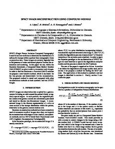
Figure 6: Frame rates across number of samples taken at preprocessing.
the hull. This occurs because increasing the number of (uniformly distributed) samples forces them to lie closer to one another and share a higher number of polygons. The LH-brain showed the highest reductions in average polygon count. This is due to the fact that this model has a high number of polygons occluded by the visible ones for any given viewpoint. Figure 6 shows the frame rates (as frames per second) observed for the three models. The first column on the x-axis shows the original frame rates for the models (3.87, 14.0, 17.7, frames/sec for LH-brain, B-gear and Bunny, respectively). The original models were rendered without applying any culling technique. The models were also rendered using hardware-supported back-face culling. In this case the frame rates remained the same as those of the original models. This is probably due to the efficiency of current graphics hardware when rendering display lists (see section 4.1). The LH-brain model allowed for the most dramatic increase in performance: up to 5.5 times the original (to 21.25 frames/sec), this is explained by the reduction in polygon count present in the reconstructions. B-gear also presented a significant improvement: 2.55 times the original (to 35.8 frames/sec). The speed-up for the Bunny was 1.4 times the original frame rate (to 24.5 frames/sec). The reason for the difference in improvement rates is that Bunny doesn’t have as much self-occlusion as the other two models.
The results in Figure 5 show that the number of rendered polygons can be greatly reduced (26%, 53% and 70% ) with respect to the original models using 25 samples.
Figure 7 shows the histograms of the pixels missed in the view reconstructions of the three models with respect to the original images for an arbitrary viewpoint. Image size was 255x255 pixels and pixel intensity varied from 0 to 1. The images used for the histogram of figure 7 are shown in Figure 8, which shows images generated using a base set of 25 IB-samples.
Results also indicate that a higher number of samples increases the percentage of culled polygons for each face in
These results were obtained on an SGI Onyx2 Infinite Reality, with 2 195MHz MIPS R10000 CPUs and video out-
Figure 5: Percentages of average culling across number of samples taken at preprocessing.
c The Eurographics Association 2001.
Meruvia and Strothotte / ID-Bitfields
other hand, our technique is simple to set up and implement, general for any polygonal model, and can be used within model hierarchies as will be shown in the next section. However, it cannot deal with extremely large model databases, because there is no hardware implementation that permits efficient memory use when the reconstructed views are computed for each face of the convex hull.
Missed pixels across pixel intensities 40 Number of Pixels 35 30 25 20 15
5. Conclusions and Future Work
10 5 0 0
Bunny
255 0
B-Gear
255 0
LH-Brain
255
Figure 7: Histograms of the differences between the three original models and their reconstructed views across pixel intensity. Total missed pixels are 23, 294 and 623 pixels for each model respectively.
put at 72.00Hz. The system was programmed using OpenGL and Open Inventor and the current implementation has no special requirements neither in hardware nor in the graphics library, since the views are generated before interaction. 4.1. Comparison with other techniques A well known culling technique that can be compared to ours is the back-face test. To make a fair comparison between our technique and back-face culling we need to analyze the implementation of both algorithms. In each case, the system goes through the list of polygons and tests each polygon. For the back-face test, the system tests each polygon’s normal against the vector between the current viewpoint and the center of projection, and computes the angle between these two vectors, if the angle is greater than 90 degrees, the polygon is back facing and is discarded. For the bitfield test, the graphics system requires to retrieve the bit from the bitfield, and inspect the value of the bit. Both tests occur in linear time, but the number of operations is less for the bitfield test. In addition, the pointer to the relevant byte of the bitfield can be kept while traversing the bitfield, or the whole bitfield can be placed in a cache, thus the decision can be done with few instructions. Conservative occlusion culling techniques (see Section 2) are superior in the sense that they are more general: they work for arbitrary viewpoints close and inside of the model or scene, and they require more preprocessing of static scenes, by means of database construction and voxelization of the model space. In many cases depth maps and depth hierarchies are computed for each viewpoint, and all polygons in the model need to be tested against this hierarchy and the viewing frustum to ensure that all visible polygons will be sent to the renderer. These techniques are used to process scenes or models with millions of polygons and achieve frame rates of 12 frames/sec in average 10 6 . On the c The Eurographics Association 2001.
A technique to achieve real-time visualization of approximate view reconstructions has been presented. The technique is based on the selection of precomputed viewdependent samples of an object. These samples consist of a bitfield indicating the visible polygons and the camera parameters where the sample was taken. The reconstruction of the view is non-conservative, since some visible polygons may be missing in the reconstructed views. Results show that reconstructed IB-samples can be used to improve system responsiveness in interactive systems that use models with high depth complexity. Future work can be divided in two areas: optimization of the current technique and visualization of other model representations. The following improvements are proposed: * Patch-Bitfields. A way to improve the ID-Bitfields is to group those polygons which lie in the same neighborhood into polygonal patches and assign them a unique ID at the bitfield. These groups of polygons can be efficiently compiled into polygon lists and the length of the ID-bitfields would be smaller, since there would only be one bit per polygon patch. Additionally, the current duplication of information in the display lists would be eliminated, since a small set of polygon patches can be combined in real-time. This reduction of duplicated information can drastically reduce the set-up time required for the technique, allowing for a more efficient use of the ID-Bitfields. * Development of a selection node for a scene graph or an object hierarchy. A selection node works in scene graphs as a node that selects one of the children based on state information (e.g. distance to the viewpoint) from the graphics system. IB-samples can be implemented in a scene graph using selection nodes, where selection depends on the viewing matrix and the nodes to be selected are the different views. This would permit appropriate view reconstruction of hierarchical models, which are widely spread in current graphics systems. * The bitfield representation can be optimized by compressing the bitfield for storage. In this paper bitfields are saved as a sequence of 32-bit integers. In many cases, depending on the way that polygons are distributed inside the (source) indexed polygon array, whole sections of the bitfield are filled with zeros. These sections are the ideal candidates for compression when saved on disk. When using the bitfield during execution, a hierarchical
Meruvia and Strothotte / ID-Bitfields
encoding of the bitfield could be computed to do a faster traversal for individual bit queries. For example, when an integer of the bitfield has value zero, we know that all values inside the bitfield are zero and need not query those individual values any more. * Implementation in the graphics library. Comparisons with other algorithms, such a back-face culling (section 4.1) suggest that if the application was allowed to pass an IDbitfield, rendering time could be improved, since the bit test is simple and can be implemented in hardware. The generic nature of the ID-bitfield could spark new applications for it. * Application for Non-realistic images. Non-realistic images are normally time-consuming to compute, and they are highly view-dependent. Shading parameters, stroke styles and direction of strokes can vary for any specific viewpoint. For the purposes of this paper, the goal of a non-realistic viewer is to pre-compute as much information as possible so the visualization for arbitrary viewpoints can be done in real-time. * Development of a navigation viewer. So far the viewer allows viewing at any distance and from any direction outside of the object (without level-of-detail handling). Under this extension the user would be able to visualize the inner sections of an object or scene. To do this, a space partitioning algorithm would be necessary to determine the boundaries of the 3D cells. In a similar way to the visualization algorithms based on cell partitioning 5 10 , the set of visible polygons could be precomputed for each viewing cell, and the set could be extended to the set of neighboring cells as well, to guarantee smooth transitions between cells. As mentioned before, the technique here presented is compatible with most of the existing occlusion culling applications. The encoding and visualization approach presented here can also be used as a post-processing step once complex scenes have been rendered and need to be replayed as is the case of virtual walkthroughs where path trajectories are predetermined and used frequently. This technique could also be applied to level-of-detail hierarchies to reduce the number of visible polygons during interaction.
2.
Saito, T., Takahashi, T. Comprehensible rendering of 3-D shapes. SIGGRAPH 90 Conference Proceedings, 197–206, 1990. 2
3.
Bourke, P. Sphere Generation. http://www.swin.edu.au/ astronomy/pbourke/modelling/sphere/ 3
4.
Coorg, S., Teller, S. Real-Time Occlusion Culling for models with Large Occluders. Symposium on Interactive 3D Graphics, 1997, 83–90, 1997. 3
5.
Darsa L, Costa Silva, B., Varshney, A. Navigating Static Environments Using Image-Space Simplification and Morphing. Symposium on Interactive 3D Graphics, 1997, 25–34, 1997. 2, 8
6.
Durand, F., Drettakis, G., Thollot, J., Puech, C. Conservative Visibility Preprocessing Using Extended Projections. SIGGRAPH 2000 Conference Proceedings, 239-248, 2000. 3, 7
7.
Shoemake, K. Arcball Rotation Control. Graphics Gems IV, 175–192. Academic Press, Boston, 1994. 3
8.
Shade, J., Lischinski, D., Salesin, D., DeRose, T., Snyder, J. Hierarchical Image Caching for Accelerated Walkthroughs of Complex Environments. SIGGRAPH 96 Conference Proceedings, 75–82, August 1996. 2
9.
Shade,J., Gortler, S. J., He, L.W., Szeliski, R. Layered Depth Images. SIGGRAPH 98 Conference Proceedings, 231–242, July 1998. 2
10. Zhang, H., Manocha, D., Hudson, Tom., Hoff III, K. Visibility Culling using Hierarchical Occlusion Maps. SIGGRAPH 97 Conference Proceedings, 77–88, August 1997. 3, 7, 8
Acknowledgments The authors would like to thank Lourdes Castillo for carefully proof-reading this paper and making appropriate suggestions. The LH-brain model was provided by Thomas Witzel. This work was supported by a Scholarship of the University of Magdeburg, Germany. References 1.
Deussen, O., Strothotte,Th. (Ed.) Pixel-Oriented Rendering of Line Drawings. Computational Visualization Graphics, Abstraction and Interactivity, 105–120. Springer-Verlag, 1998. 2 c The Eurographics Association 2001.
Meruvia and Strothotte / ID-Bitfields
Figure 8: View reconstruction of LH-brain (top), B-gear and Bunny. Original models are shown on the left, reconstructed views are shown on the right. During preprocessing, 25 IB-samples were taken for each of the models. c The Eurographics Association 2001.