each internal node is labeled by an attribute and its branches are labeled by the ... rithm, where rK is a suitably defined Ramsey number with a known bound.
Approximating Decision Trees with Multiway Branches Venkatesan T. Chakaravarthy, Vinayaka Pandit, Sambuddha Roy, and Yogish Sabharwal IBM India Research Lab, New Delhi, India {vechakra,pvinayak,sambuddha,ysabharwal}@in.ibm.com
Abstract. We consider the problem of constructing decision trees for entity identification from a given table. The input is a table containing information about a set of entities over a fixed set of attributes. The goal is to construct a decision tree that identifies each entity unambiguously by testing the attribute values such that the average number of tests is minimized. The previously best known approximation ratio for this problem was O(log2 N ). In this paper, we present a new greedy heuristic that yields an improved approximation ratio of O(log N ).
1
Introduction
In many situations (such as machine fault detection, medical diagnosis, species identification), one is required to identify an unknown entity (among a possible set of known entities), by performing a sequence of tests. Typically, each test is restricted to checking the value of an attribute of the unknown entity. Naturally, one wishes to design a testing procedure that minimizes the expected number of tests needed to identify the unknown entity. As an example, consider a typical medical diagnosis application. A hospital maintains a table containing information about diseases. Each row represents a disease and each column is a medical test and the corresponding entry specifies the outcome of the test for a person suffering from the given disease. When the hospital receives a new patient whose disease has not been identified, it would like to determine the shortest sequence of tests which can unambiguously determine the disease of the patient. Motivated by such applications, the problem of constructing decision trees for entity identification from given data, has been well studied (See the surveys by Murthy [1] and Moret [2]). In this paper, we present an improved approximation algorithm for the above problem, when the tests are multi-valued. Decision Trees for Entity Identification - Problem Statement. The input is a table D having N rows and m columns. Each row is called an entity and the columns are the attributes of these entities. A solution is a decision tree in which each internal node is labeled by an attribute and its branches are labeled by the values that the attribute can take. The entities are the leaves of the tree. The tree should identify each entity correctly. The goal is to construct a decision tree in which the average distance of a leaf from the root is minimized. Equivalently, S. Albers et al. (Eds.): ICALP 2009, Part I, LNCS 5555, pp. 210–221, 2009. c Springer-Verlag Berlin Heidelberg 2009 �
Approximating Decision Trees with Multiway Branches
A
B
1
1
1
e2
1
2
0
e3
1
e4
2
4
0
e5
2
4
1
e6
2
5
0
3
A
C
e1
1
2
B
1
Input Table
211
1 e1
2 e2
B
B 3
4
5
e3
1 e1
C
e6 0 e4
2 e2
3 e3
5
4 e6
1 e5
A Decision Tree of cost 14
C 0
e4
1 e5
Optimal Decision Tree of Cost 8
Fig. 1. Example decision trees
we want to minimize the total external path length defined as the sum of the distances of all the entities to the root. We call this the DT problem. Example: Figure 1 shows an example table and two decision trees. The total external path length of the first tree is 14 and that of the second (optimal) tree is 8. An equivalent way of computing the cost is to sum over the internal nodes v, the number leaves under v. For instance, in the first tree, the cost can be computed as 6 + 3 + 3 + 2 = 14 and for the second tree, it is 6 + 2 = 8. � � A special case of the DT problem is when every attribute can take only two values (say {0, 1}); this restricted version is called the 2 − DT problem. In general, for some K ≥ 2, if every attribute is restricted to take at most K distinct values (say {0, 1, . . . , K − 1}), we get the K − DT problem. The general DT problem has no such restriction on the possible values of attributes. Hyafil and Rivest [3] showed that the 2 − DT problem is NP-Hard. Garey [4] presented a dynamic programming based algorithm for the 2 − DT problem that finds the optimal solution, but the algorithm runs in exponential time in the worst case. Kosaraju et al. [5] studied the 2−DT problem and showed that a popular greedy heuristic gives an O(log N ) approximation. Adler and Heeringa [6] gave an alternative proof and improved the approximation ratio by a constant factor to (1 + ln N ) (See also [7]). Garey and Graham [8] showed that the natural greedy algorithm considered in [5,6] has approximation ratio Ω(log N/ log log N ). Chakaravarthy et al. [9] studied the K − DT problem and gave an rK (1 + ln N )-approximation algorithm, where rK is a suitably defined Ramsey number with a known bound that rK ≤ 2 + 0.64 log K; thus, their approximation ratio is O(log K log N ). On the hardness front, they also showed that the 2 − DT problem and the general DT problem cannot be approximated within factors of 2 and 4 respectively unless NP=P. The weighted version of the DT problem has also been studied. Here, there is a probability distribution associated with the set of entities and the goal is to minimize the expected path length. (The unweighted version that we defined corresponds to the case where the distribution is uniform). The O(log N )-approximation algorithm by Kosaraju et al. [5] can also handle the
212
V.T. Chakaravarthy et al.
weighted 2 − DT problem. For the weighted K − DT problem, Chakaravarthy et al. [9] gave a O(log K log N )-approximation algorithm. On the hardness front, it is known that the weighted 2 − DT problem cannot be approximated within a factor of Ω(log N ), unless NP=P [9]. In the general DT problem, K can be very large (up to N ), in which case the approximation ratio of [9] is O(log2 N ). So, a natural question is whether there exists an approximation algorithm for the general DT problem matching the approximation ratio of O(log N ) for the 2 − DT problem. In this paper, we present an algorithm with an approximation ratio of O(log N ) for the general (unweighted) DT problem based on a new greedy heuristic. We now mention the main ingredients of our algorithm and its analysis. Essentially, each internal node of a decision tree narrows down the possibilities for the unknown entity. The greedy heuristic considered in [9], at each internal node, chooses the attribute that maximizes the number of pairs separated (two entities are said to be separated if they do not take the same branch). In contrast, the greedy heuristic that we propose chooses an attribute which minimizes the size of the heaviest branch. In the case of the 2 − DT problem, these two heuristics are equivalent. One of the central ideas used in the analysis of [5] is that of “centroidal path”. Our main insight lies in drawing a connection between the notion of centroidal path and the objective function of the Minimum Sum Set Cover (MSSC) problem [10]. This insight allows us to utilize some ideas from the analysis of the greedy algorithm for the MSSC problem by Feige et al. [10]. It is interesting to note that the hardness results in [9] are obtained via reductions from the MSSC problem. In this paper, we utilize the MSSC problem in the other direction, namely we use ideas from the analysis of the greedy algorithm for the MSCC problem to obtained improved upper bounds on the approximation ratio. Our analysis, in its current form, does not extend to the weighted DT problem. It would be interesting to obtain a O(log N ) approximation algorithm for the weighted DT problem as that would give matching upper and lower bounds for the problem.
2
Preliminaries
In this section, we define the DT problem and develop some notations. Let D be a table having N rows and m columns. Each row is called an entity and each column is called an attribute. Let E denote the set of all N entities and A denote the set of m attributes. For e ∈ E and a ∈ A, denote by e.a the value taken by e on attribute a. We are guaranteed that no two entities are identical. For a ∈ A, let Va denote the set of values taken by the attribute a. Let K = maxa |Va |. We have K ≤ N . For instance, if the table is binary, K = 2. A decision tree T for the table D is a rooted tree satisfying the following properties. Each internal node u is labeled by an attribute a and has at most |Va | children. Every branch (edge) out of u is labeled by a distinct value from the set Va . The entities are the leaves of the tree and thus the tree has exactly N leaves. The tree should identify every entity correctly. In other words, for any
Approximating Decision Trees with Multiway Branches
213
entity e, the following traversal process should correctly lead to e. The process starts at the root node. Let u be the current node and a be the attribute label of u. Take the branch out of u labeled by e.a and move to the corresponding child of u. The requirement is that this traversal process should reach the entity e. Observe that the values of the attributes are used only for taking the correct branch during the traversal. So, we can map each value of an attribute to a distinct number from 1 to K and assume that Va is a subset of {1, 2, . . . , K}. Therefore, we assume that for any e ∈ E and a ∈ A, e.a ∈ {1, 2, . . . , K}. Let T be a decision tree for D. For an entity e ∈ E, path length of e is defined to be the number of internal nodes in the path from the root to e; it is denoted �T (e) (Note that this is the same as the number of edges on the path). The sum of all path lengths is called total path length and is denoted cost(T ), i.e., cost(T ) = Σe∈E �T (e). We say that e pays a cost of �T (e) in T . DT Problem: Given a table D, construct a decision tree for D having the minimum cost. Remark: In general, we can define a decision tree for any subset of entities of the table (E ⊆ E) and its cost will be defined analogously.
3
Greedy Algorithm
In this section, we describe our greedy algorithm. Let D be the input table over N entities E and m attributes A. Consider a subset of entities E ⊆ E and an attribute a ∈ A. The coverage of a on E is defined as below. The attribute a partitions the set E into K parts, given by Ej = {e ∈ E : e.a = j}, for 1 ≤ j ≤ K. Let j ∗ be denote the part having the largest size, i.e., j ∗ = argmaxj |Ej |. We say that a covers all the entities in E, except those in Ej ∗ and define � Ei Cover(E, a) = i∈({1,2,...,K}−j ∗ )
The entities in Ej ∗ are said to be left uncovered. We note that some of the set Ej could be empty. The greedy algorithm works as follows. For the root of the decision tree, we pick the attribute � a having the maximum coverage; equivalently, we minimize the size of the heaviest branch (containing the uncovered entities). The attribute � a a = i}. We recursively apply partitions E into E1 , E2 , . . . EK , where Ei = {e : e.� the greedy procedure on each of these subsets and get the required decision tree (See Figure 2). Let T� denote the decision tree obtained by this procedure. Let Topt denote the optimal decision tree for D. We claim that the greedy algorithm has an approximation ratio of 4 log N . The theorem is proved in the next section. Theorem 1. The greedy algorithm has an approximation ratio of 4 log N , meaning cost(T� ) ≤ (4 log N )cost(Topt ).
214
V.T. Chakaravarthy et al.
Procedure Greedy(E) Input: E ⊆ E , a set of entities in D; Output: A decision tree T for the set E Begin If E is empty, Return an empty tree. If |E| = 1, Return a tree with x ∈ E as a singleton node. Let � a be the attribute that covers the maximum number of entities: � a = argmaxa∈A Cover(E, a) Create the root node r with � a as its attribute label. For 1 ≤ j ≤ K, a = j} Let Ej = {e ∈ E|e.� Tj = Greedy(Ej ) Let rj be the root of Tj . Add a branch from r to rj with label j and join Tj to T . Return T with r as the root. End Fig. 2. The Greedy Algorithm
4
Analysis of the Greedy Algorithm: Proof of Theorem 1
We extend the notion of cost to all subtrees of the greedy tree T� . Consider an internal node v ∈ T� and let T�v be the subtree rooted at v. Let L(v) denote the entities (or leaves) in T�v ; these are the entities that appear below v in T�. For instance, if r is the root of T�, then T� = T�r and L(r) = E. Let I(T�v ) denote the internal nodes of T�v . Define � (length of path from v to e). cost(T�v ) = e∈L(v)
Here, length refers to the number of internal nodes in the path from v to e. Remark: Notice that T�v is the output of the greedy procedure, if L(v) is the input set of entities. We say that v handles the set of entities given by L(v). Proposition 1. For any internal node v ∈ T , cost(T�v ) = Σx∈I(T�v ) |L(x)|. Proof. Consider an entity e ∈ L(v). Let � be the length of the path from v to e; this is the cost contributed by e in cost(Tv ). Note that there are � internal nodes on this path. We charge a unit cost to each of these internal nodes. Then, the charge accumulated at each internal node x is exactly |L(x)|. The proposition follows by summing up these accumulated charges over all the internal nodes � � of T�v . The following proposition is useful in proving Theorem 1. Proposition 2. Let E ⊆ E be a set of entities. Let E1 , E2 , . . . , Ed be any disjoint subsets of E. Let T1∗ , T2∗ , . . . Td∗ be the optimal decision trees for E1 , E2 , . . . , Ed , respectively and let T ∗ be the optimal decision tree for E. Then, cost(T1∗ ) + cost(T2∗ ) + · · · + cost(Td∗ ) ≤ cost(T ∗ ).
Approximating Decision Trees with Multiway Branches
215
Proof. Consider any Ei . We can construct a decision tree Ti for Ei from T ∗ as follows. Remove from T ∗ any entity (i.e, leaf) not appearing in Ei ; iteratively remove any internal node having no children. Cleary, the resulting tree Ti is a decision tree for Ei . For any entity e ∈ Ei , the cost paid by e in Ti is the same as the cost paid by e in T ∗ . Since Ei ’s are disjoint, we have that cost(T1 ) + cost(T2 ) + · · · + cost(Td ) ≤ cost(T ∗ ). � �
The lemma now follows directly.
We shall prove following lemma which generalizes Theorem 1. For a subset of entities E ⊆ E, let TE∗ denote the optimal decision tree for E. Consider an ∗ internal node u ∈ T� . TL(u) is the optimal decision tree for L(u). Theorem 1 is obtained by applying the following lemma to the root node r of T� . ∗ ) where Lemma 1. For any internal node u ∈ T� , cost(T�u ) ≤ (4 log n)cost(TL(u) n = |L(� u)|.
Proof. The lemma is proved by induction on the number of internal nodes in the subtree under consideration. If T�u has only one internal node, then each entity pays a cost of 1; this is optimal. Now, let us prove the inductive step. We state some important definitions first. An internal node x of T� is said to be terminal, if all its children are leaves. For a non-terminal internal node x of T� , its centroidal child is defined to be the child of x having the maximum number of leaves (breaking ties arbitrarily). We now extend this to the notion of centroidal path. Consider the subtree T�v rooted at some internal node v of T� . Starting at the root node of T�v (i.e., the node v), iteratively keep picking the centroidal child till we reach an internal node having only leaves as its children. Such a path is called the centroidal path of T�v and is denoted by Cent(T�v ). Cost of the centroidal path is defined as � |L(x)|. cost(Cent(T�v )) = �v ) x∈Cent(T
Remark: It is easier to visualize the centroidal path if we make the centroidal child of each node as the right most child. Then, the Cent(T�v ) will be the right extreme path starting at v. We now prove the inductive step in Lemma 1. Consider an internal node u. ∗ ), where n = |L(u)| We wish to show that cost(T�u ) ≤ (4 log n)cost(TL(u) Cost of T�u can be decomposed into two parts by considering cost incurred along the centroidal path of T�u and the remaining cost. We say that an internal node v of T�u is adjacent to the centroidal path Cent(T�u ), if v is not part of the centroidal path, but it is a child of some node in the centroidal path. Let Adj denote the set of all nodes adjacent to Cent(T�u ). Then, the cost of T� can expressed as below; the expression follows from Proposition 1. � cost(T�v ). (1) cost(T�u ) = cost(Cent(T�u )) + v∈Adj
216
V.T. Chakaravarthy et al.
Consider any v ∈ Adj. Since v is a non-centroidal node, we have |L(v)| ≤ n/2. Moreover, the number of internal nodes in T�v is less than that of u. Thus, by the inductive hypothesis, we have that ∗ cost(T�v ) ≤ 4 log(n/2)TL(v) .
(2)
In Lemma 2 (see Section 5), we show that ∗ ) cost(Cent(T�u )) ≤ 4cost(TL(u)
(3)
Assuming the above bound, we can complete the proof of Lemma 1. So, � cost(T�v ) (from Eqn. 1) cost(T�u ) = cost(Cent(T�L(u) )) + ≤
∗ ) 4cost(TL(u)
+
�
v∈Adj
cost(T�v )
(from Eqn. 3)
∗ 4 log(n/2)cost(TL(v) )
(from Eqn. 2)
v∈Adj ∗ ≤ 4cost(TL(u) )+
�
v∈Adj ∗ ∗ ) + 4 log(n/2)cost(TL(u) ) ≤ 4cost(TL(u)
(from Prop. 2, taking E = L(u)) ≤
∗ 4 log(n)cost(TL(u) )
We have completed the proof of Lemma 1 and hence, Theorem 1, assuming Lemma 2. � �
5
Bound on the Centroidal Cost
In this section, we will prove the following lemma. ∗ ). Lemma 2. For any internal node u ∈ T� , cost(Cent(T�u )) ≤ 4cost(TL(u)
Proof. Let us start by simplifying the notation. Consider any internal node u ∈ T� . Let T� = T�u be the greedy subtree rooted at u. and let E = L(u) be the entities handled by T�. Notice that T� is nothing but the tree constructed by the ∗ be the optimal greedy algorithm, if E is the set of input entities. Let T ∗ = TL(u) ∗ � tree for E. Our goal is to argue that cost(Cent(Tu )) ≤ 4cost(T ). Let r be the length of Cent(T�) and let the nodes on the path be u1 , u2 , . . . , ur . For 1 ≤ i ≤ r, write Ei = L(ui ). Let a1 , a2 , . . . ar be the attributes associated with u1 , u2 , . . . , ur , respectively. Consider a node ui , for some 1 ≤ i < r. Let Ci = Cover(Ei , ai ); we say that ui covers the entities in Ci . The node ur is a boundary case, and is handled separately. The children of ur are all leaves and these are given by Er . Recall that Cover(Er , ar ) includes all the entities in Er , except one. For the node ur , we define Cr = Er . Note that each entity in E is covered by exactly one node among u1 , u2 , . . . , ur . See Figure 3(a); here, r = 4.
Approximating Decision Trees with Multiway Branches
v1 u1 E1 a1
∗ E1
v2
∗ RC1
u2 E2 a2 C1
∗ E2
v3
b3
∗ E3
v4
∗ RC3
u4 E4 a4
C3
b2
∗ RC2
u3 E4 a3
C2
b1
217
∗ RC4
C4
(a)
b4
∗ E4
Orphan
(b)
Fig. 3. Centroidal paths of the greedy and the optimal tree
Remark: Each node ui handles the set of entities given by Ei . The node splits Ei into two parts: the set Ci covered by ui and the set Ei+1 handled by ui+1 . An alternative way to view cost(Cent(T�)) is as follows. Each entity in Ci pays a cost of i. Now, cost(Cent(T�)) is the sum of the cost paid by all the entities, �r i.e., cost(Cent(T�)) = i=1 i|Ci |. The above function is similar to the objective function in the MSSC problem. This connection allows us to utilize ideas from the analysis of the greedy algorithm for MSSC by Feige et al. [10]. r |Ei |. Recall that the cost of the centroidal path cost(Cent(T�)) is given by Σi=1 Consider a node ui , for some 1 ≤ i ≤ r. We imagine that the node ui pays a cost of |Ei | towards the centroidal cost. Distribute this cost equally among the entities covered by ui : for each e ∈ Ci , define its price pe = Notice that
|L(ui )| |Ci |
cost(Cent(T�)) =
�
pe .
e∈E
Now, let us consider the optimal tree T ∗ . For each entity e ∈ E, let �∗ (e) denote length of the path from the root to e in T ∗ ; this is viewed as the cost paid by e in T ∗ . Recall that cost(T ∗ ) = Σe∈E �∗ (e). We will now bound the price paid by any entity e in the greedy solution T� by the cost paid by some entity e∗ in the optimal solution T ∗ (within a factor of two). For this, we define a mapping π : E → E that maps entities in T� to entities in T ∗ such that an entity e in T� will charge its price pe to the entity π(e) in T ∗ . Our mapping π will satisfy the following two properties: 1. For any entity e∗ ∈ E, there are at most two entities mapped to it (i.e., |{e : π(e) = e∗ }| ≤ 2). 2. For any entity e ∈ E, pe ≤ 2�∗ (π(e)).
218
V.T. Chakaravarthy et al.
Lef t∗ = P red ∩ R e∗1
e∗ 2
e∗3
σ∗ : e∗4 e∗5
Pred π(e)
σ∗ e∗6
e∗7
e∗8 C1
e1
e2
e3
e4
e5 σ:
e6
e7
e8
(a)
C2
C3
σ e
C4
C5
R
(b) Fig. 4. Illustration of the mapping π and Left ∗
We call such a mapping to be nice. We shall exhibit a nice mapping π in Section 6. Given such a mapping, we can now see that cost(Cent(T�)) ≤ 4cost(T ∗ ). This completes the proof of Lemma 2. � �
6
A Nice Mapping
In this section, we exhibit a nice mapping π claimed in the proof of Lemma 2. We arrange the nodes in E in the order in which they are covered by the nodes u1 , u2 , . . . , ur . Namely, first place all the nodes in C1 (in some arbitrary order), followed by those in C2 and so on, finally ending with those in Cr . Let this ordering be denoted σ = e1 , e2 , . . . en (where n = |E|). In this ordering, the entities come in blocks: first C1 , then C2 and so on, ending with Cr . Now, let us consider the optimal tree T ∗ . Arrange the entities in ascending order of cost �∗ (·) they pay in T ∗ . Namely, all the entities that pay a cost of 1 (if any) are placed first (in some arbitrary order), followed by those paying a cost of 2 (if any) and so on. Let this ordering by denoted as σ ∗ = e∗1 , e∗2 , . . . , e∗n . In σ ∗ , as we scan from left to right, the cost paid by the entities increases monotonically. We now define the mapping π as follows. Scan the lists σ and σ ∗ from right to left, picking two entities from σ and mapping them both to a single entity in σ ∗ . Formally, if e is an entity appearing in position i from the right in σ, it will be attached to the entity appearing in position i/2 from the right in σ ∗ . See Figure 4(a). Clearly, every entity in σ ∗ has at most two entities from σ mapped to it. Thus, the mapping π satisfies the Part (1) of the niceness property. Now, we shall show that π also satisfies Part (2) of the niceness property. 6.1
Bounding Greedy Price
In this section, we will show that for any entity e in σ, p(e) ≤ 2�∗ (π(e)). We will use the following notations. Consider any subset of entities S ⊆ E. We extend the notion of coverage considering only the entities in S and define the concept of CoverS (·, ·). Let X ⊆ E be a subset of entities and a be an attribute. The attribute a partitions
Approximating Decision Trees with Multiway Branches
219
the entities X into X1 , X2 , . . . , XK , where Xj = {e ∈ X : e.a = j}. Let Xj � be set among these that has the maximum size, taking only entities in S into account; meaning, let j � = argmaxi |Xi ∩ S|. Then, CoverS (X, a) is defined to include every set Xi , except Xj � : CoverS (X, a) =
�
(Xi ∩ S)
i∈({1,2,...,K}−j � )
Consider the optimal tree T ∗ and S ⊆ E be some subset of entities. In T ∗ , we define the notion of centroidal path with respect to S. For any internal node y ∈ T ∗ , let L(y) be the leaves in the subtree rooted at y. By considering only those entities in S, we get LS (y); i.e., define LS (y) = L(y) ∩ S. Consider an internal node v ∈ T ∗ . Among the children of v, let y be node having the maximum value of LS (y) (breaking ties arbitrarily); such a y is called the S-centroidal child of v. The S-centroidal path of T ∗ is defined next: starting with the root node of T ∗ , we traverse the tree by picking up the S-centroidal child in each step, until we reach some node y in which the entities in LS (y) are all children of y. We are now ready to prove the Part (2) of the niceness property. Lemma 3. For any entity e in σ, �∗ (π(e)) ≥ p(e)/2. Proof. Consider some entity e in σ. Let uh be the node covering e, so that e ∈ Ch . Recall that uh lies on the centroidal path of T�. It handles the entities Eh = ∪ri=h Ci . If h < r, uh splits Eh into Ch (which it covers) and Eh+1 = ∪ri=h+1 Ci . Let R = Eh . Note that pe = |R|/|Ch |. Let s be the length of R-centroidal path of T ∗ and let v1 , v2 , . . . , vs be nodes appearing on the path. For 1 ≤ i ≤ s, let Ei∗ = L(vi ) be the entities handled by vi . Let b1 , b2 , . . . , bs be the attributes associated with these nodes. We next define the coverage obtained by each node along the R-centroidal path. For 1 ≤ i ≤ s, define RCi∗ = CoverR (Ei∗ , bi ). Consider 1 ≤ t ≤ s. We say that the node vt covers all the entities in RCt∗ and that each entity α ∈ RCt∗ is said to be covered in the time-step t. The last node vs presents a boundary case. The entities in LR (vs ) are all children of vs ; among these all, except one, are included in RCs∗ and covered by vs ; we call the excluded entity as orphan in T ∗ . So, all entities in σ ∗ , except the orphan, are covered by node vi . See Figure 3(b); here s = 4. Let Left ∗ is the entities in R that appear before π(e) in σ ∗ . Formally, let Pred be the set of all entities that appear before π(e) in σ ∗ (including π(e)). Then, Left ∗ = Pred ∩ R. See Figure 4(b). Observation 1: Notice that for any entity e� ∈ Left ∗ , �∗ (e� ) ≤ �∗ (π(e)) (since, cost of entities in σ ∗ is monotonically increasing). We now present an outline of the proof. Intuitively, we will show the following three claims: (i) |Left ∗ | ≥ |R|/2; (ii) an entity covered in time-step t pays a cost of at least t in T ∗ ; (iii) in each time-step t, the optimal tree T ∗ can cover at most |Ch | entities from R. It would follow that it takes at least |R|/(2|Ch |) time-steps to cover Left ∗ . Therefore, some entity in Left ∗ pays a cost of at least
220
V.T. Chakaravarthy et al.
|R|/(2|Ch |). From Observation 1, it follows that �∗ (π(e)) ≥ |R|/(2|Ch |). We now formally prove the claims. Claim 1: |Left ∗ | ≥ R/2 . Proof. Since e ∈ Ch and R = ∪ri=h Ci , we have that at most R entities (including e) appear to the right of e in σ. By the definition of the mapping π, we have that in σ ∗ , at most R/2 entities appear to the right of π(e) including π(e). Thus, in σ ∗ , at most R/2 − 1 entities appear to the right of π(e) excluding π(e). It � � follows that |Left ∗ | ≥ R/2� + 1 ≥ R/2 . Claim 2: Consider any 1 ≤ t ≤ s. Any entity α covered in the time-step t in T ∗ must satisfy �∗ (α) ≥ t. Proof. To reach to root of T ∗ , α must climb up along the first t nodes of the R-centroidal path. � � Claim 3: For 1 ≤ t ≤ s, at most |Ch | entities from R can be covered in timestep t, i.e, |RCt∗ | ≤ |Ch |. Proof. The claim is proved using the fact that the greedy procedure picked attributes that give maximum coverage. Refer to Figure 5 for an illustration. Recall that LR (vt ) ⊆ R is the entities from R handled by vt and bt is the attribute as∗ sociated with vt . The attribute bt partitions LR (vt ) into X1∗ , X2∗ , . . . , XK , where ∗ ∗ ∗ Xi = {α ∈ LR (vt ) : α.bt = i}. Let j = argmaxi |Xi |. Then, note that � Xi∗ . RCt∗ = i∈{1,2,...,K}−j ∗
By contradiction, suppose |RCt∗ | > |Ch |. It is easy to see that the union of ∗ contains at least |Ch | entities. any K − 1 distinct sets from X1∗ , X2∗ , . . . , XK In the greedy tree, imagine what would happen if we picked bt (instead ah ) as the attribute at the node uh to split R = Eh . Let the partition obtained be Y1 , Y2 , . . . , YK , where Yi = {α ∈ R : α.bt = i}. So, Cover(R, bt ) is the union of some K − 1 distinct subsets from Y1 , Y2 , . . . , YK . Note that Xi∗ ⊆ Yi , for all 1 ≤ i ≤ K. Therefore, Cover(R, bt ) is a superset of the union of ∗ . This implies that |Cover(R, bt )| > some K − 1 subsets from X1∗ , X2∗ , . . . , XK |Ch |. This contradicts the fact that greedy’s choice of ah has the maximum coverage. � � The proof proceeds intuitively as follows. By Claim 3, at most Ch entities from R are covered in each time step. Since Left ∗ ⊆ R, it follows that at most Ch entities in Left ∗ are covered in each time step. Therefore, it takes at least |Left ∗ |/|Ch | time-steps to cover all the entities in Left ∗ . Since |Left ∗ | ≥ R/2 (by Claim 1), ∗ it takes at least �R/2� |Ch | steps to cover all the entities in Left . Thus, by Claim 2, some entity in Left ∗ pays a cost of at least ∗
|R| 2|Ch | .
�|R|/2� |Ch | )
≥
|R| 2|Ch | .
From Observation
1, it follows that � (π(e)) ≥ The only issue in the above argument is that by definition, orphan is not said to be covered by any node. This is a problem if orphan belongs to Left ∗ .
Approximating Decision Trees with Multiway Branches
vt bt
X1∗
X2∗
LR (vt ) ⊆ R
∗ XK
Xj∗
221
R
uh bt
Y1
RCt∗
Y2
YK
Yj�
Cover(R, bt )
(a)
(b)
Fig. 5. Illustration for Claim 3 of Lemma 3
However, this needs only a minor argument. Notice that orphan pays a cost of at least s. Recall that any internal node of the R-centroidal path of T ∗ can cover at most |Ch | entities from R. Therefore at most s|Ch | entities of R can be covered in s time-steps. But, in the s time-steps all the entities in R, except the orphan get covered. Therefore, s|Ch | ≥ R − 1 and hence, s ≥ (R − 1)/|Ch |. It follows that s ≥ R/(2|Ch |), for R ≥ 2. It is assured that R ≥ 2, since ur is an internal R . Thus, node of T� and therefore, has at least two children. Therefore, s ≥ 2|C h| ∗ R orphan pays a cost of at least 2|Ch | . Since orphan is in Left , by observation 1, we conclude that �∗ (π(e)) ≥
|R| 2|Ch |
= pe /2.
� �
References 1. Murthy, S.: Automatic construction of decision trees from data: A multidisciplinary survey. Data Mining and Knowledge Discovery 2(4), 345–389 (1998) 2. Moret, B.: Decision trees and diagrams. ACM Computing Surveys 14(4), 593–623 (1982) 3. Hyafil, L., Rivest, R.: Constructing optimal binary decision trees is NP-complete. Information Processing Letters 5(1), 15–17 (1976) 4. Garey, M.: Optimal binary identification procedures. SIAM Journal on Applied Mathematics 23(2), 173–186 (1972) 5. Kosaraju, S., Przytycka, M., Borgstrom, R.: On an optimal split tree problem. In: Workshop on Algorithms and Data Structures (1999) 6. Adler, M., Heeringa, B.: Approximating optimal binary decision trees. In: Goel, A., Jansen, K., Rolim, J.D.P., Rubinfeld, R. (eds.) APPROX and RANDOM 2008. LNCS, vol. 5171, pp. 1–9. Springer, Heidelberg (2008) 7. Heeringa, B.: Improving Access to Organized Information. Ph.D. thesis, University of Massachusetts, Amherst (2006) 8. Garey, M., Graham, R.: Performance bounds on the splitting algorithm for binary testing. Acta Informatica 3, 347–355 (1974) 9. Chakaravarthy, V., Pandit, V., Roy, S., Awasthi, P., Mohania, M.: Decision trees for entity identification: approximation algorithms and hardness results. In: ACM Symposium on Principles of Database Systems (2007) 10. Feige, U., Lov´ asz, L., Tetali, P.: Approximating min sum set cover. Algorithmica 40(4), 219–234 (2004)