approximation algorithm for the k minimum spanning tree ... - CiteSeerX

An O(log k) approximation algorithm for the k minimum spanning tree problem in the plane Naveen Garg

Dorit S. Hochbaumy

Abstract

Given points in the Euclidean plane, we consider the problem of nding the minimum tree spanning any points. The problem is NP-hard and we give an (log )-approximation algorithm. n

k

O

k

1 Introduction A cable company is permitted to service k cities in a state with n cities. To minimise the cost of installation the company wishes to nd a set of cities that are \close". Since we need to connect these cities, a natural measure of \closeness" is the weight of the minimum tree spanning them where the weight of the edge (i; j ) is the euclidean distance, d(i; j ), between cities i and j . More formally, the problem that we address in this paper is the following.

Problem k-EMST Given n points in the Euclidean plane, nd the minimum weight tree spanning at least k points.

The motivation for the problem arose in bidding for licenses to operate oil rigs within contiguous regions. That application and a facility layout application are described by Fischetti, Hamacher, Jornsten and Maoli in [5]. They also prove that the problem is NP-hard. Ravi, Sundaram, Marathe, Rosenkrantz and Ravi [12] showed that it is NP-hard to compute the minimum weight tree spanning k points in the plane. Note that the problem is polynomially solvable for xed k; for every set of k points we compute the minimum tree spanning the set and pick the set for which the weight of this tree is minimum. The problem is polynomial when the underlying graph is a tree [9]. In [6] there is a further study of the problem on general graphs, and some integer programming formulations and solution techniques are demonstrated. Ravi et.al. [12] were the rst to establish an approximation worst case bound for the problem. Their paper describes an algorithm that achieves an approximation factor of O(k1=4). It also gives a polynomial time exact solution for the special case when the points are on the boundary of a convex region in the plane.  y

Max-Planck-Institut fur Informatik, Im Stadtwald, 66123 Saarbrucken, Germany Industrial Engineering and Operations Research, University of California, Berkeley, CA 94720

1

The main result of this paper is an O(log k) approximation to the k-EMST problem. We use a family of rectangular grids to identify the set of k points. The set of points we pick is such that they occupy only a small number of cells in each grid. We show that for a particular choice of grids this implies that the minimum tree spanning the point set is small. Subsequent to the rst appearance of this paper, there has been signi cant progress in improving the approximation guarantee for this log k ) by Eppstein [4], to O(1) by Blum, problem. The approximation factor was improved p to O( loglog n Chalasani and Vempala [3] and more recently to 2 2 by Mitchell [10].

2 Related problems The problem of computing the minimum tree spanning any k points can be viewed in the general setting of nding a \best" subgraph spanning k vertices and satisfying certain properties. Clearly, all problems for which the properties can be checked in polynomial time are polynomially solvable for xed k, by examining all k point subsets. In particular if we require that the subgraph be connected and of the least possible weight, then we are really looking for the minimum p weight tree that spans k vertices; an extension of the k-EMST problem to general graphs. A 3 k-approximation algorithm for this problem was rst given by [12] and this has been improved recently to a O(log2 k)-approximation algorithm by Awerbuch, Azar, Blum and Vempala [2]. If the subgraph we are looking for is the one with the maximum weight then the problem is NPhard as the k-clique problem can be reduced to it [13]. The best known approximation ratio for this heaviest subgraph problem is O~ (n0:3885) and is due to Kortsarz and Peleg [8]. For trees the problem can be solved in time O(nk2 ) using dynamic programming [7]. Similar to the heaviest subgraph problem is the lightest induced subgraph problem where we wish to pick k vertices such that the subgraph induced is of the minimum weight. Once again this problem is NP-hard (the k-independent set problem can be reduced to it); the geometric version of this problem has been studied in [1] and the graph version in [11].

3 Lower bounds An important issue in the design of approximation algorithms for optimization problems is that of the bounding technique used. For the purpose of analysing the algorithm we need to compare the cost of its solution to the optimum. But since, computing the value of the optimum is itself NP-hard we need a lower bound on the optimum (assuming a minimisation problem) against which we can compare our solution. Further, this lower bound should be close to the optimum; if for instance, optimum value  
(lower bound), then any approximation algorithm that uses this lower bounding technique can at best guarantee an approximation factor of . Thus, we need to look for good lower bounding techniques that mimic the optimum. We rst discuss two lower bounding techniques due to [12]. Our technique can be viewed as a re nement of these lower bounds.

2

3.1 Diameter Let V be the set of n points and V   V be the k points picked by the optimum. We denote by d(i; j ) the Euclidean distance between points i and j . The diameter of a set, S  V , is the maximum distance between any two points of S and is denoted by diam(S ). For every pair of points p i; j construct a circle Cij with center as the midpoint of line segment (i; j ) and diameter  = 3d(i; j ). This choice of center and diameter ensures that the circle corresponding to the farthest points1 of V  contains all of V  . Let Cpq be the circle with the minimum diameter that contains at least k points. Clearly, d(p; q )  diam(V  )  weight of minimum tree spanning V . Thus, d(p; q) is aplower bound on the weight of the minimum tree spanning k points. [12] show how to obtain an O( k) approximation using this lower bounding technique. A disadvantage of this lower bounding technique is that the lower bound is always less than the diameter of the optimum point set, V  . Thus if V  were such that the minimum tree spanning V  was large compared to diam(V  ) then we would have a large gap between the optimum value and the lower bound. This, for example, would be the case when V  is a set of evenly spaced points in a square. The next lower bounding technique, also due to [12], takes care of this shortcoming.

3.2 The Grid Lemma 3.1 ([12]) Consider a rectangular grid, G, each cell of which is a square of side x. If t is the minimum number of cells containing k points then the minimum weight tree spanning any k points has weight (tx).

Ravi et.al. [12] combine this lower bound with diameter considerations and obtain an O(k1=4) approximation to the optimum. Note that if the optimum point set V  is such that all points of V  are contained in a small number of cells of G but these cells are far apart, then the value of this lower bound could be much less than the optimum. We obtain a better lower bound by considering grids of dierent cell sizes.

4 The Approximation Algorithm The algorithm works by \guessing" for each pair of points, that they are the furthest away in the optimal solution set. For every pair of pointspi; j construct a circle Cij with center as the midpoint of the line segment (i; j ) and diameter  = 3d(i; j ). This choice of center and diameter ensures that any point set for which (i; j ) are the farthest points lies completely within Cij . Let Qij be a square of side  circumscribing Cij . If p; q are the farthest points in the optimal point set V , then all points of V  are contained in Qpq . Thus, it suces to solve the problem independently in each square Qij (by restricting ourselves to the points contained in the square) and then p picking the minimum tree. From now on we limit our discussion to the square Qpq of side  = 3d(p; q ). For the sake of brevity we denote this square by Q and let V denote the set of points contained in it. If p; q are the two farthest points in V  and v is another point in V  then d(v; p)  d(p; q). Also, p d(v; q )  d(p; q ) and therefore the distance of v from the midpoint of the line segment joining p and q is at most 23 d(p; q) 1

3

We need to nd a set of k points in Q that are \close", in the sense that the weight of the minimum tree spanning the points is small. To this end we de ne a potential function on the point set, P : 2V ! R+. Our choice of potential is such that a set of points is \close" if its potential is small. Let Gi be a rectangular grid in Q, each cell of which is a square of side xi . The size of grid Gi is the size of its cell i.e xi .

De nition 4.1 The Gi-potential of a set S  V , denoted by Gi(S ), is equal to xiti where ti is the number of cells of Gi that contain points of S .

As remarked earlier this de nition of potential is not sucient as we could have a set of k points that are contained in only a few cells of Gi which, however, are far apart. This set of points has a small potential with respect to this grid even though the minimum tree spanning this set is large. To take care of this we de ne the potential of a set with respect to a collection of grids.

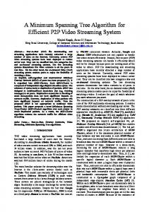
Figure 1: Grids

G 0 ; G1 ; G2

Note that any set of points has a potential  with respect to the square Q. Further, the Gi -potential of any set of k points is less than  if grid Gi has a size less than k . Hence, we get no advantage by considering a grid of size less than k in our family of grids. Let G0 be a rectangular grid of size x0 = k in Q. De ne Gi to be the grid, each cell of which is a square composed of four cells of grid Gi?1 . If xi denotes the size of Gi then xi = 2xi?1 = 2i x0. Since xlog k = 2log k x0 = kx0 =  , Glog k is the square Q2. Thus we have log k dierent grids G0; G1 : : :Glog k?1 . Figure 1 shows grids G0; G1 and G2 drawn with dotted, dashed and solid lines respectively.

De nition 4.2 The potential of a set S is the sum of the Gi-potentials of S i.e. P (S ) =

X

log k?1 i=0

Gi(S )

Our algorithm essentially nds a set of k points with the minimum potential and computes the minimum tree spanning the points. 2 Throughout this paper we assume that k is a power of 2; for general k all arguments apply with log k replaced by dlog ke.

4

Algorithm E-MST(k); for all pairs of points i; j do 1. Construct a circle centered at thepmidpoint of the line segment (i; j ) with diameter  = 3d(i; j ).

2. if circle contains at least k points then fLet Q be a square of side  circumscribing the circle. g 2.1. S  = minpot(Q) f nd set with minimum potential in Q g 2.2. Compute the minimum tree spanning S 

Output the minimum weight tree found in Step 2.2 and the set S  corresponding to it.

end.

In Section 6 we show a polynomial time algorithm for the procedure minpot(Q) which, given the square Q nds a set of k points in Q that has the minimum potential. In the next section we prove, formally, our claim that the potential of a point set is small i the weight of the minimum tree spanning this set is small and show how this leads to the O(log k) approximation factor.

5 The approximation guarantee We rst show that a \close" set of points has a small potential.

Lemma 5.1 If V  is the optimum point set then P (V ) =

X

log k?1 i=0

Gi (V  )  8 log k
OPT

where OPT is the weight of the minimum tree spanning V  .

Proof: Consider a grid Gi of size xi and let ti cells of this grid contain all the points of V . We rst prove that the Gi -potential of V  , Gi (V  ), is at most 8
OPT. We have two cases depending on the value of ti . 1. ti  4 p p Since the coarsest grid has a size of 2 , xi  2 . Also,  = 3d(p; q )  3
OPT and therefore

p Gi (V ) = xiti  2  2 3
OPT < 8
OPT

2. ti > 4 We color the cells of the grid as follows: assign every cell a color depending on whether the row/column that the cell belongs to is odd/even. Since these are four dierent possibilities we use only 4 dierent colors and no two cells that are adjacent or diagonally adjacent have the same color. Since the points of V  lie in ti cells, there are at least t4 cells that contain points from V  and belong to the same color class. To connect two cells from the same color i

5

Figure 2: Building the spanning tree class requires an edge of length at least xi . Hence the tree spanning V  must have length at least xi ( t4 ? 1) which, since ti > 4, is at least x8t . Therefore i

i i

Gi (V  ) = xiti  8
OPT

Since Gi (V  )  8
OPT for every grid Gi , 0  i  log k ? 1, the Lemma follows. The following Lemma proves the converse i.e. that a set of points with a small potential is \close".

Lemma 5.2 The minimum tree spanning any set, S , of k points has weight at most p P log k?1 2( i=0 Gi(S )). Proof: We show this by constructing a tree spanning S of weight no more than the claimed bound. The tree is built in a hierarchical manner; we rst connect all points of S contained in a cell of grid G0 and then add edges across cells of G0 to connect points of S in a cell of G1 and so on (Figure 2). We begin with the grid G0 and for each cell of this grid pick a tree over the points of S contained in the cell. Consider a cell p containing m points of S . Since no edge picked has length p more than the diameter of the cell ( 2x0 ) the total weight of edges picked p from this cell is 2x0(m ? 1). Hence the total weight of edges picked from all cells is at most 2x0 (k ? t0 ) where t0 is the number of cells of G0 containing points from pS . But x0 t0 = G0(S ) and therefore the weight of edges picked p in this step is 2(x0 k ? G0 (S )) = 2( ? G0 (S )). Our algorithm for connecting points of S proceeds in iterations. At the start of the ith iteration all points of S contained in a cell of Gi?1 are connected. In this iteration we add edges across cells of Gi?1 so as to ensure that for each cell of Gi, all points of S contained in the cell are connected.

p Claim 5.1 The total weight of edges picked in the ith iteration is at most 2(2Gi?1(S ) ? Gi(S )).

Proof: Consider a cell of Gi . Of the four cells of Gi?1 contained in this cell of Gi , let m (0  m  4), cells contain points from p S . Thus we need to add m ? 1 edges; each edge is ofp weight at most the diameter of the cell ( 2xi ). Thus the weight of edgesppicked from this cell is 2xi (m ? 1). Hence, the total weight of edges picked from all cells of Gi is 2xi (ti?1 ? ti ), where ti?1 ; ti are the number 6

of cells in Gi?1 ; Gi respectively that contain points from S . Since xi = 2xi?1 , the total weight picked in this step is at most

p

p

2xi (ti?1 ? ti ) = p2(2xi?1 ti?1 ? xi ti ) = 2(2Gi?1 (S ) ? Gi (S ))

Thus by the endpof log k iterations we have a tree spanning all points of S . The total weight of this tree most 2( ? G0 (S ) + 2G0 (S ) ? G1 (S ) + : : : + 2Glog k?1 (S ) ? Glog k (S )), which is equal to p Pislogatk?1 2 i=0 Gi (S ). This completes the proof of Lemma 5.2. Having proven that a set of points has a small potential i it has a small tree spanning it (Lemmas 5.1 and 5.2) we now show that the minimum tree spanning S  has weight at most O(log k) OPT. Recall that S  is a set of k points from Q with the minimum potential. Since the optimal point set, V , is also contained in Q, P (S  )  P (V  ) and therefore

p

weight of minimum tree spanning S   p2P (S )  p2P (V )  8 2 log k
OPT = O(log k)
OPT The only thing that now remains is to nd the set S  in polynomial time.

6 Finding the set with minimum potential In this section we show a polynomial time algorithm for nding a \close" set of k points with the minimum potential. Our algorithm uses Dynamic Programming to identify this set. Consider a cell in grid Gi and associate with this cell a list, L, of k elements. The pth element in this list is the minimum total potential with respect to grids G0 ; G1 : : :Gi of any set of p points contained in this cell. Formally, Xi G (S ) L(p) = min j S :jS j=p j =0

where S is contained in the cell of Gi being considered. Note that the 0th element of any list is always zero. The lists for cells of G0 can be constructed immediately. If a cell of G0 contains m points then the elements L(1); L(2) : : :L(m) are set to x0 while the remaining elements are assigned a suitably large value, say 1. Given lists for cells of Gi?1 we can obtain the list for a cell in grid Gi in the following manner. Consider the four cells of Gi?1 that make up this cell of Gi . To obtain the pth element we need to nd the best way of splitting p (p = p1 + p2 + p3 + p4 ) such that picking p1; p2; p3; p4 points respectively from these four cells minimises the total potential with respect to grids G0 ; G1 : : :Gi?1 . This minimisation can be done in polynomial time by considering all 4-partitions of the number p and using the lists for cells of Gi?1 to nd the total potential with respect to grids G0; G1 : : :Gi?1 7

for each partition. The pth element for the cell of Gi is then the sum of this value and xi , the potential with respect to grid Gi . Thus, for p  1, L(p) = p1 ;pmin fL1(p1) + L2(p2) + L3(p3) + L4(p4)g + xi 2 ;p3 ;p4

where p1 + p2 + p3 + p4 = p and L1; L2; L3; L4 are lists for the four cells of Gi?1 contained in this cell. The list L, can be computed more eciently in O(k2 ) time as follows. L(p) = L1 (p) L(p) = 0min L(i) + L2 (p ? i) ik L(p) = 0min L(i) + L3 (p ? i) ik L(p) = 0min L(i) + L4 (p ? i) ik and for p  1

L(p) = L(p) + xi

procedure minpot(Q); for all cells of G0 do for p := 1 to k do if cell contains more than p points then L(p) = x0

else

L(p) = 1 for i := 1 to log k do for all cells of Gi do

end.

Compute list L.

Lemma 6.1 The kth element in the list for Q corresponds to a set of points with the minimum potential.

Proof: Let S  be the set of points corresponding to the kth element in the list for Q. By the manner in which we have de ned the lists it follows that S  has the minimum total potential with respect to grids G0; G1 : : :Glog k from amongst any set of k points contained in Q, i.e.

X G (S )  logXk G (S )

log k i=0

i

i=0

i

where jP S j = jS j = k and S  V . Since, Glog k (S ) =  for any set  6= S  V , S  also minimises k?1 P (
) = log Gi (
) and therefore is a set with minimum potential. i=0 Since the total number of cells in all the grids put together is 12 + 22 + 42 + : : : + k2 = O(k2 ), and computation of each list takes O(k2) time, the procedure minpot() has a running time complexity of O(k4 ). 8

7 A Tight Example The example given here illustrates that the log k gap between the lower and upper bounds is in fact attainable for a family of problems. In this paper we use the diameter and the grid lower bounds to arrive at an O(log k)-approximation to the k-EMST problem. This diers from [12] in that instead of considering just one grid, as in [12], we consider a collection of log k grids and look at the average lower bound with respect to these grids for every collection of k points. An alternative strategy would be to look at the maximum lower bound provided by any one of these log k grids since this would be at least as large as the average. The following example (Figure 3) is a collection of k points in a square of side  such that each of the log k grids provides exactly the same lower bound, i.e.  , and the weight of the minimum tree spanning these points is  log k. This shows that considering the maximum lower bound provided by any grid is no better than considering the average. The points are arranged so that each cell of Gi which contains any points has them in exactly two cells of Gi?1 . This implies that ti = 2k and so the potential of this set of points with respect to each grid is exactly  . Let the four cells of Gi?1 in a cell of Gi be numbered 1,2,3,4 in a clockwise order starting at the top-left cell. Further, we distribute the points so that the two cells of Gi?1 that the points of Gi are contained in are the cells numbered 2 and 4 if i is even and 1 and 3 if i is odd. This gives an arrangement of points as shown in Figure 3 and it is easy to see that the minimum steiner tree spanning these points is of length O( log k). i

Figure 3: A tight example

8 On a variant of the travelling salesman problem We now consider an interesting variant on the travelling salesman problem. Consider a travelling salesman who wishes to visit the maximum number of cities on a given amount of fuel. The bound on the fuel is equivalent to placing a bound on the total distance travelled by the salesman. Once again we assume that the cities are points in a plane and the distance between two cities is the euclidean distance between the corresponding points. More formally, 9

Problem Given n points in the Euclidean plane and a bound B, nd a cycle of length

at most B that includes the maximum number of points.

It is easy to see that this variant on the Euclidean travelling salesman problem is NP-hard as well. In this section we present an O(log n)-approximation algorithm for this problem. Note that the minimum tree spanning a set of points and the minimum tour on these points are related as

MST (S )  TSP (S )  2
MST (S ) where MST (S ) (resp. TSP (S )) denotes the minimum tree (resp. tour) spanning the points in the set S . We use this fact as follows. Let B be the bound on the length of the tour that we are looking for and b the number of points in the optimum tour. Then the minimum tree spanning p b points is of length at most B and hence our algorithm would nd a tree of length at most 8 2 log b
B . We can now short-circuit thisptree to obtain a tour of length at most p twice the length of the tree. We now divide this tour into 32 2 log b segments, each having b=(32 2 log b) vertices. Clearly one of the segments has length no more than B and we can complete this segment into a tour of length at most B . Thus we have a tour of length 2 p no more than B and containing at least b=(16 2 log b) vertices, where b is the maximum number of vertices that any tour of this length can contain. Since b  n, we obtain a O(log n)-approximation to this variant of the travelling salesman problem. Since we do not the value of b in advance, we run the above procedure for all possibe choices of b (n in all) and output the best solution. Acknowledgements We wish to acknowledge useful discussions with R. Ravi, Madhu Sudan and Randeep. We also wish to thank Vempala Santosh for suggesting the travelling salesman problem variant and H. Ramesh for the tight example in Figure 3.

References [1] A. Aggarwal, H. Imai, N. Katoh, and S. Suri. Finding k points with minimum diameter and related problems. Journal of Algorithms, 12(1):38{56, 1991. [2] Baruch Awerbuch, Yossi Azar, Avrim Blum, and Santosh Vempala. Improved approximation guarantees for minimum weight k-trees and prize-collecting salesmen. In Proceedings, 27th Annual ACM Symposium on Theory of Computing, pages 277{283, 1995. [3] Avrim Blum, Prasad Chalasani, and Santosh Vempala. A constant-factor approximation for the k-mst problem in the plane. In Proceedings, 27th Annual ACM Symposium on Theory of Computing, pages 294{302, 1995. [4] D. Eppstein. Faster geometric k-point mst approximation. Technical Report 13, University of California, Irvine, CA, 1995. [5] M. Fischetti, H.W. Hamacher, K. Jornsten, and F. Maoli. Weighted k-cardinality trees: complexity and polyhedral structure. Networks, 24:11{21, 1994. [6] M. Fischetti, H.W. Hamacher, and F. Maoli. Weighted k-cardinality trees. Technical Report 23, Politecnico di Milano, 1991. 10

[7] O. Goldschmidt and D.S. Hochbaum. k-edge subgraph problems. Manuscript, 1994. [8] G. Kortsarz and D. Peleg. On choosing a dense subgraph. In Proceedings, 34th Annual IEEE Symposium on Foundations of Computer Science, 1993. [9] F. Maoli. Finding a best subtree of a tree. Technical Report 41, Politecnico di Milano, 1991. [10] J.S.B. Mitchell. Guillotine subdivisions approximate polygonal subdivisions: a simple new method for the geometric k-mst problem. In Proceedings, 7th Annual ACM-SIAM Symposium on Discrete Algorithms, pages 402{408, 1996. [11] V. Radhakrishnan, S. Krumke, M.V. Marathe, D.J. Rosenkrantz, and S.S. Ravi. Compact location problems. In Proceedings, 13th Conference on Foundations of Software Technology and Theoretical computer science, pages 238{247, 1993. [12] R. Ravi, R. Sundaram, M.V. Marathe, D.J. Rosenkrantz, and S.S. Ravi. Spanning trees short and small. In Proceedings, 5th Annual ACM-SIAM Symposium on Discrete Algorithms, 1993. [13] S.S. Ravi, D.J. Rosenkrantz, and G.K. Tayi. Facility dispersion problems: Heuristics and special cases. In Proceedings, 2nd Workshop on Algorithms and Data Structures, 1991.

11