introduced by Revannaswamy and Bhatt [69] as an extension to this .... Three exact-solution algorithms for the DCMST problem, developed by ..... d , the expected value of the diameter for a labeled tree with n nodes, is given by: n n d n n nd d.
COMPUTING A DIAMETER-CONSTRAINED MINIMUM SPANNING TREE
by
AYMAN MAHMOUD ABDALLA B.S. Montclair State University, 1992 M.S. Montclair State University, 1996
A dissertation submitted in partial fulfillment of the requirements for the degree of Doctor of Philosophy in the School of Electrical Engineering and Computer Science in the College of Engineering and Computer Science at the University of Central Florida Orlando, Florida
Spring Term 2001
Major Professor: Narsingh Deo
ABSTRACT
In numerous practical applications, it is necessary to find the smallest possible tree with a bounded diameter. A diameter-constrained minimum spanning tree (DCMST) of a given undirected, edge-weighted graph, G, is the smallest-weight spanning tree of all spanning trees of G which contain no path with more than k edges, where k is a given positive integer.
The problem of finding a DCMST is NP-complete for all values of k;
4 ≤ k ≤ (n – 2), except when all edge-weights are identical. A DCMST is essential for the efficiency of various distributed mutual exclusion algorithms, where it can minimize the number of messages communicated among processors per critical section. It is also useful in linear lightwave networks, where it can minimize interference in the network by limiting the traffic in the network lines. Another practical application requiring a DCMST arises in data compression, where some algorithms compress a file utilizing a tree data-structure, and decompress a path in the tree to access a record. A DCMST helps such algorithms to be fast without sacrificing a lot of storage space. We present a survey of the literature on the DCMST problem, study the expected diameter of a random labeled tree, and present five new polynomial-time algorithms for an approximate DCMST. One of our new algorithms constructs an approximate DCMST in a modified greedy fashion, employing a heuristic for selecting an edge to be added to
the tree in each stage of the construction.
Three other new algorithms start with an
unconstrained minimum spanning tree, and iteratively refine it into an approximate DCMST. We also present an algorithm designed for the special case when the diameter is required to be no more than 4. Such a diameter-4 tree is also used for evaluating the quality of other algorithms. All five algorithms were implemented on a PC, and four of them were also parallelized and implemented on a massively parallel machine—the MasPar MP-1. heuristics.
We discuss convergence, relative merits, and implementation of these
Our extensive empirical study shows that the heuristics produce good
solutions for a wide variety of inputs.
iii
To my parents
iv
ACKNOWLEDGEMENTS
First of all, thank God for the abilities and opportunities that made this dissertation possible.
I would like to thank my advisor, Prof. Narsingh Deo, for his guidance and
assistance, which significantly contributed to the further development of my research and writing skills. I would also like to thank the committee members: Profs. Robert Brigham, Mostafa Bassiouni, Ronald Dutton, and Ali Orooji, whose comments helped me improve this dissertation. I would like to give special thanks to my parents, and the rest of my family, who gave me unconditional support and encouragement throughout the course of my studies. Also, thanks to my fiancé, who has been very supportive and understanding during the long time I needed to conduct research and write this dissertation. Last but not least, thanks to all my friends and colleagues, especially those in the Center for Parallel Computation, for their comments and encouragement, and thanks to the staff of the School of Electrical Engineering and Computer Science for all their help.
v
TABLE OF CONTENTS
LIST OF FIGURES ...................................................................................................... viii LIST OF SYMBOLS ...................................................................................................... ix CHAPTER 1: INTRODUCTION ................................................................................... 1 1.1 Motivation ..................................................................................................... 2 1.2 Existing Algorithms for the DCMST Problem ............................................. 6 1.3 A Generalization of the DCMST Problem .................................................. 11 1.4 Related Optimization and Decision Problems ............................................ 12 1.5 Diameter Sets and the Dynamic DCMST ................................................... 14 1.6 The Diameter of a Random Tree ................................................................. 16 1.7 Outline ......................................................................................................... 17 CHAPTER 2: EXPECTED VALUE OF MST-DIAMETER .................................... 19 2.1 Exact Average-Diameter ............................................................................. 21 2.2 Approximate Average-Diameter ................................................................. 27 CHAPTER 3: QUALITY OF AN APPROXIMATE DCMST .................................. 30 3.1 Polynomially-Solvable Cases ..................................................................... 30 3.2 The Special-Case Algorithm for DCMST(4) .............................................. 32 CHAPTER 4: THE IR1 ITERATIVE-REFINEMENT ALGORITHM .................. 35 4.1 The Algorithm ............................................................................................. 35 4.2 Implementation ........................................................................................... 41 4.3 Convergence ................................................................................................ 42 CHAPTER 5: THE IR2 ITERATIVE-REFINELENT ALGORITHM ................... 43 5.1 Selecting Edges for Removal ...................................................................... 47 5.2 Selecting a Replacement Edge .................................................................... 49 5.2.1 Edge-Replacement Method ERM1 ........................................... 49 5.2.1 Edge-Replacement Method ERM2 ........................................... 51 5.3 Implementation ........................................................................................... 53 5.4 Convergence ................................................................................................ 57
vi
CHAPTER 6: THE CIR ITERATIVE-REFINELENT ALGORITHM .................. 60 6.1 Implementation ........................................................................................... 60 6.2 Convergence ................................................................................................ 62 CHAPTER 7: THE ONE-TIME-TREE-CONSTURCTION ALGORITHM .......... 64 7.1 The Algorithm ............................................................................................. 64 7.2 Implementation ........................................................................................... 68 7.3 Convergence ................................................................................................ 70 CHAPTER 8: PERFORMANCE COMPARISONS .................................................. 72 CHAPTER 9: CONCLUSION ...................................................................................... 77 APPENDIX A: PROGRAM CODE FOR COMPUTING EXACT AVERAGEDIAMETER ......................................................................................... 79 APPENDIX B: PROGRAM CODE FOR THE ITERATIVE-REFINEMENT ALGORITHMS ................................................................................... 88 APPENDIX C: PROGRAM CODE FOR THE ONE-TIME-TREECONSTURCTION ALGORITHM .................................................. 119 LIST OF REFERENCES ............................................................................................ 151
vii
LIST OF FIGURES
2.1
The unlabeled trees of order 6 ................................................................................. 20
2.2
Different ways to connect a node from S 2 to a node in S 1 .................................... 25
2.3
Percentage error in approximate average-diameter ................................................ 27
3.1
One step in constructing an approximate DCMST(4) from DCMST(3) ................ 33
4.1
An example of cyc ling in IR1 ................................................................................. 36
4.2
Finding an approximate DCMST(2) by penalizing 2 edges per iteration ............... 38
5.1
An example of IR2 .................................................................................................. 44
5.2
Weight quality of approximate solution, in randomly weighted complete-graphs with Hamiltonian-path MSTs, produced by IR2 using two different edgereplacement methods ............................................................................................... 53
8.1
The ratio ((spanning-tree weight) / (MST weight)) in randomly weighted completegraphs ...................................................................................................................... 73
8.2
The ratio ((spanning-tree weight) / (MST weight)) in randomly weighted completegraphs with Hamiltonian-path MSTs ...................................................................... 74
8.3
The ratio ((spanning-tree weight) / (MST weight)) in randomly weighted graphs with 20% density ..................................................................................................... 75
8.4
The time required by different algorithms to obtain an approximate DCMST(5) in randomly weighted complete-graphs ...................................................................... 76
viii
LIST OF SYMBOLS
∀
the universal quantifier
|S|
the number of nodes in tree S, (if S is a tree), or the number of elements in set S (if S is a set).
β
the bandwidth of a line in a network
∆
the maximum node-degree in the tree
ε
a small positive constant
ρ
number of leaves adjacent to a given bicenter node in a tree of diameter 3
Θ(g(n))
bounded by g(n)
Ω(g(n))
bounded below by g(n)
a, b, c
nodes
a1 , a2 , ai, aσ diameters from a tree-diameter set, described in Chapter 1 Adj(v)
nodes adjacent to v within the given set of edges
BFST
breadth-first spanning tree
C
the set of edges near the center of the spanning tree
CIR
the composite-iterative-refinement algorithm
d
the diameter of a spanning tree
Dd (x)
the enumerator (generating function) for all trees with diameter d
dn
the expected value of diameter for a labeled tree with n nodes
DCMST
diameter-constrained minimum spanning tree
ix
DCMST(k)
diameter-constrained minimum spanning tree with diameter no more than k
dist(u, v)
the (unweighted) distance from node u to node v
distc(l)
the distance of edge l from the center of the tree, plus 1
dists(i)
the distance from the source node (or edge) to node i
e
Napier’s constant ≈ 2.71828⋅⋅⋅
E, E’, E*
sets of edges
ecc(u)
the eccentricity of node u: the maximum distance from node u to any node in the same tree
eccT(u)
the eccentricity of node u with respect to tree T
ERM1, ERM2 the edge-replacement methods used by Algorithm IR2 G, G’, G*
graphs
Gh (x)
the enumerator (generating function) for all trees with height ≤ h
h
the height of a tree
Hh (x)
the enumerator (generating function) for all trees with height = h
hv
a function that determines the candidate “Hubs” in the algorithm developed by Paddock and described in Chapter 1
i i
[in Chapter 2] a subscript [in all chapters except for Chapter 2] a node
IR1
the first general-iterative-refinement algorithm
IR2
the second general-iterative-refinement algorithm
j
a node
k
the given constant-bound on diameter
l
an edge
L
the lightest excluded-edge in the algorithm developed by Paddock and described in Chapter 1
x
lc
the center edge of a tree of odd diameter
lij, lsj
boolean decision variables, used in the mixed-integer-linear-programming formulation developed by Achuthan et al. and described in Chapter 1
ln n
the natural logarithm (logarithm base e) of n
log n
the logarithm of n with any constant base
m
the number of edges in the given graph
m1, m2, mh
variables
M(P)
a problem of finding the smallest tree isomorphic to prototype P
MAX{…}
the maximum of two or more values
MAX {...}
the maximum of values calculated for all a in set A
MIN {...}
the minimum of values calculated for all a in set A
MIPS
million instructions per second
MST
minimum spanning tree
n
the number of nodes in the given graph
near(u)
a tree node candidate to be incident to u in the approximate DCMST
a∈ A
a∈A
NSM1, NSM2 node-selection methods used with Algorithm OTTC NSM3
a node-selection method used with Algorithm OTTC
O(g(n))
bounded above by g(n)
OTTC
the one-time-tree-construction algorithm
p
the number of processes allowed to be executing in their critical section at the same time
P
a prototype
q
the number of selected start nodes in Algorithm OTTC
r
the radius of a graph
xi
s
a source node in a directed graph
SIMD
single instruction-stream over multiple data-streams
t
the time required to traverse a link in a network
t n (h)
the number of labeled rooted-trees with n nodes, a specified root, and height no more than h
Tv
a breadth-first spanning tree
Tγ
a tree from a sequence
〈Tγ〉
a sequence of trees
u, v
nodes
V, V’
sets of nodes
vc
the center node of a tree of even diameter
W〈u, v〉
the weight of the directed edge from u to v
W(u, v)
the weight of edge (u, v)
W(T)
the weight of tree T
w1 , w2 , … ,wn weights of edges, also used in referencing edges wmax
the largest edge-weight in the current spanning tree
wmin
the smallest edge-weight in the current spanning tree
X
a bitmap vector
x x
[in Chapter 2] a variable (used in generating functions) [in all chapters except for Chapter 2] a node
y, z, z0
nodes
xii
CHAPTER 1 INTRODUCTION The Diameter-Constrained Minimum Spanning Tree (DCMST) problem can be stated as follows: given an undirected, edge-weighted graph, G, and a positive integer, k, find a spanning tree with the smallest weight among all spanning trees of G which contain no path with more than k edges. The length of the longest (unweighted) path in the tree is called the diameter of the tree. This problem was shown to be NP-complete by transformation from the Exact Cover by 3-Sets problem [33]. Let n denote the number of nodes in G. It can be easily shown that the problem can be solved in polynomial time for the following four special cases: k = 2, k = 3, k = (n – 1), or when all edge weights are identical. As stated in [33], the other cases are NP-complete, even when edge weights are randomly selected from the set {1, 2}. We consider G to be connected; where the edge-weights of G are non-negative numbers, randomly chosen with equal probability, following the Erdös-Rényi model [28].
1
1.1 Motivation
The DCMST problem has applications in several areas, such as in distributed mutual exclusion, linear lightwave networks, and bit-compression for information retrieval.
In
distributed systems, where message passing is used for interprocessor communication, some algorithms use a DCMST to limit the number of messages.
For example,
Raymond's algorithm [22, 66] imposes a logical spanning tree structure on a network of processors.
Messages are passed among processors requesting entrance to a critical
section and processors granting the privilege to enter.
The maximum number of
messages generated per critical-section execution is 2d, where d is the diameter of the spanning tree. Therefore, a small diameter is essential for the efficiency of the algorithm. Minimizing edge weights reduces the cost of the network. A fault-tolerant protocol was introduced by Revannaswamy and Bhatt [69] as an extension to this algorithm.
The
protocol makes the algorithm tolerant to single node/link failure and associated network partition. This is done by utilizing non-tree edges without increasing the upper bound on the number of passed messages. Satyanarayanan and Muthukrishnan [74] modified Raymond's original algorithm to incorporate the “least executed” fairness criterion and to prevent starvation, also using no more than 2d messages per process.
In a subsequent paper [75], they presented a
distributed algorithm for the readers and writers problem, where multiple nodes need to access a shared, serially reusable resource.
In this distributed algorithm, the number of
2
messages generated by a read operation and a write operation has an upper bound of 3d and 2d, respectively. In another paper on distributed mutual exclusion, Wang and Lang [86] presented a token-based algorithm for solving the p-entry critical-section problem, where a maximum of p processes are allowed to be in their critical section at the same time. If a node owns one of the p tokens of the system, it may enter its critical section; otherwise, it must broadcast a request to all the nodes that own tokens. Each request passes at most 2pd messages. The critical section protocol presented by Seban [76, 77] keeps a bound on the logical clock using a distributed predictive “clock squashing” mechanism.
For simplicity, he
assumed a constant-size message requiring a constant time t to traverse a network link, thus modeling the network by an undirected graph. For a general graph whose spanning tree has diameter d, it takes d⋅t time to transfer a message between the two most distant nodes, and each node must process messages to and from all adjacent nodes. Therefore, the protocol has control-section access-time performance Θ(MAX{d, ∆})⋅t, where ∆ is the maximum node-degree in the tree. The worst-case performance occurs for linear and star graphs, where a star is a tree with at most one non-leaf. It is desirable to construct the spanning tree with diameter and maximum degree in O(log n), where n is the number of nodes in the graph. This problem is related to the DCMST problem, especially if the time taken by a message to traverse an edge is variable. A solution to the DCMST problem can be a spanning tree with the smallest total edge-traversal time, and diameter O(log n). If the maximum degree is not O(log n), the tree must be refined into the desired form.
3
For such cases, a new algorithm needs to be developed to refine the node degrees of the DCMST without increasing its diameter. In addition to its applications in distributed mutual-exclusion, a DCMST is useful in information retrieval, where large data structures called bitmaps are used in compressing large files.
It is required to compress the files, so that they will occupy less memory
space, while allowing reasonably fast access. Bookstein and Klein [17, 18] proposed a preprocessing stage, in which bitmaps are first clustered and the clusters are used to transform their member bitmaps into sparser ones that can be more effectively compressed. This is done by associating pairs of bitmap vectors such that the occurring of a 1-bit in a vector increases the likelihood of a 1-bit occurring in the same position in the other vector. The association is made by an XOR operation of the pair, creating a new vector with a smaller number of 1’s. The number of 1’s in the resulting cluster is called the Hamming distance between the two associated bitmap vectors.
A small
Hamming distance is desirable when compressing bitmap vectors because a smaller number of 1-bits allows more efficient compression. Between the two associated bitmap vectors, the vector with the higher number of 1’s is discarded. The other vector may be associated again, with a new bitmap vector, in the same manner.
All non-discarded
vectors and clusters are compressed. An efficient clustering method starts by generating a complete edge-weighted-graph structure on the bitmaps, where the nodes represent bitmaps, and the weighted edges represent Hamming distances. Then, the method uses a spanning tree of this graph to cluster and compress vectors along the paths from a chosen node, the root, to all the leaves of the spanning tree. To recover a given bitmap vector, X,
4
it is required to decompress all nodes in the path from the root to X.
Therefore, a
spanning tree with a small diameter can provide high-speed retrieval. However, the total Hamming distance of the spanning tree must be low in order to conserve storage space. Consequently, a DCMST provides the necessary balance between access speed and storage space. The DCMST problem also arises in linear lightwave networks, where multi-cast calls are sent from each source to multiple destinations. It is desirable to use a spanning tree with a small diameter for each transmission to minimize interference in the network. An algorithm by Bala et al. [14] decomposes a linear lightwave network into edge disjoint trees with at least one spanning tree. The algorithm builds trees with small diameters by computing trees whose maximum node-degree is less than a given parameter, rather than by optimizing the diameter directly. Furthermore, the lines of the network are assumed to be identical.
If the linear lightwave network has lines of different bandwidths, lines of
higher bandwidth should be included in the spanning trees to be used more often and with more traffic.
Employing an algorithm that solves the DCMST problem can help find a
better tree decomposition for this type of network. The network can be modeled by an edge-weighted graph, where an edge of weight 1/β is used to represent a line of bandwidth β.
5
1.2 Existing Algorithms for the DCMST Problem
Three exact-solution algorithms for the DCMST problem, developed by Achuthan et al. [5], were based on a mixed-integer-linear-programming formulation of the problem [4, 6]. Branch-and-Bound methods were used to reduce the number of subproblems. The algorithms were implemented on a SUN SPARC II workstation operating at 28.5 MIPS. The algorithms were tested on complete graphs of different orders (n ≤ 40), using 50 cases for each order, where edge-weights were randomly generated numbers between 1 and 1000. The fastest of the three algorithms with diameter bound k = 4 produced an exact solution in less than one second on average when n = 20, but it took an average of 550 seconds when n = 40. Subsequently,
Achuthan
et
al.
[7]
developed
a
better
mixed-integer-linear-
programming formulation of the DCMST problem, thus improving the three branch-andbound
algorithms.
The
improved
mixed-integer-linear-programming
formulation
distinguishes the cases of odd and even diameter-constraint, k. Let W(i, j) denote the weight of undirected edge (i, j), and W〈i, j〉 denote the weight of the directed edge from i to j. For the DCMST being constructed, let lij denote a decision variable that takes the value 1 when edge 〈i, j〉 or 〈j, i〉 is in the spanning tree, and 0 when neither edge is in the spanning tree.
When k is even, the following formulation is used to solve the DCMST
problem. Extend the given graph G = (V, E) to a directed graph G’ = (V’, E’), where V’ = V ∪ {s}, and E’ is obtained by replacing each edge (i, j) ∈ E with the directed edges
6
〈i, j〉 and 〈j, i〉, with W(i, j) = W〈i, j〉 = W〈j, i〉, and adding a zero-weight edge 〈s, u〉 for every u ∈ V.
The mixed-integer-linear-programming formulation for constructing a
DCMST with diameter no more than k is: Construct a graph G* = (V’, E* ), E* ⊆ E’, which minimizes:
∑W
f =
i , j l ij
(1.1)
i , j ∈V '
subject to the constraints:
∑l
sj
= 1,
(1.2)
j∈V
∑l
ij i ∈V ', j∈V ,i ≠ j
and
= 1,
(1.3)
dists(i) – dists(j) + (k/2 + 1)lij ≤ k/2
∀〈i, j〉 ∈ E’,
(1.4)
lij ∈ {0, 1}
∀〈i, j〉 ∈ E’,
(1.5)
0 ≤ dists(i) ≤ k/2 + 1
∀i ∈ V’,
(1.6)
where dists(i) represents the distance from node s to node i in G* . The reasoning behind this formulation is the following.
Equation 1.1 optimizes the
spanning tree weight. Conditions 1.2 and 1.3 ensure that node s has outdegree 1, and all other nodes have indegree 1. By limiting the distance from s to each node in the tree being constructed, Condition 1.4 prevents cycles from forming. Together, conditions 1.2, 1.3, and 1.4 lead to the creation of a directed graph G* , consisting of directed paths from s to all other nodes. Conditions 1.4 and 1.6 ensure that the length of each of these directed paths has length no more than (k/2 + 1). The solution, which is an exact DCMST with diameter no more than k, is the underlying undirected graph of G* – {s}.
7
When the diameter constraint k is odd, a similar formulation can be developed. The odd formulation does not require the use of an extra source node s. Rather, it chooses one directed edge 〈u, v〉 as the source edge, where dists(i) is the distance from edge 〈u, v〉 to i. The constructed graph, G* , is a tree that can be put in a layer structure such that all directed paths have u or v as their origin.
The required DCMST is the underlying
undirected graph of G* . The improved algorithms [7] were tested with the same type of graphs and on the same machine as the original algorithms.
When tested with k = 4, the fastest of the
improved algorithms produced exact solutions in 113, 366, and 7343 seconds on average for graphs of 40, 50, and 100 nodes, respectively.
Since such exact algorithms have
exponential time complexity, they are not suitable for graphs with thousands of nodes. One special-case algorithm, which computes an approximate DCMST with diameter bound k = 6, was developed by Paddock [59]. The algorithm can be described as follows. First, the edges of the graph G = (V, E) are sorted according to weight, and the smallest 20% edges are assigned to the set E’, and all other edges are deleted. In this algorithm, all missing edges are assumed to have weight 0. Then, for each node v, compute: hv =
∑
∑ ( L − W (u , z )) ,
u∈ Adj ( v ) z∈ Adj ( u )
where Adj(a) is the set of nodes x such that edge (a, x) ∈ E’, and L is the smallest edgeweight in E larger than all edge-weights in E’. Choose five nodes v having the largest hv values as the candidate “Hubs.”
Each Hub is used to generate a candidate DCMST,
where the smallest-weight DCMST among them is selected as the approximate solution. Each candidate DCMST is computed using the following greedy strategy. 8
Initialize the
tree to a Hub, then add nodes to the tree using Prim's algorithm, but at each step, use only those edges that result in a distance from the Hub of 3 or less. Once this spanning tree is obtained, refine it by replacing some of its edges, one by one, with minimum-spanningtree edges not in the current spanning tree. Each replacement is made only if it does not cause the distance from the Hub to any node to exceed 3.
The worst-case time
complexity of this algorithm is O(nm + n2 ), where n and m are the number of nodes and edges in the input graph, respectively.
This algorithm is not effective since it only
considers distances from the Hub, using a small number of Hubs, rather than using the distance between each pair of nodes in the tree being constructed.
Hence, it tries to
optimize the diameter by optimizing the radius. If the initial choice of Hub is poor, the produced solution may be significantly heavier than the optimal.
Furthermore,
generalizing this algorithm is less effective for odd values of k. A better algorithm could optimize the diameter directly, discarding fewer edges by the greedy strategy, thus making the algorithm less vulnerable to the choice of Hub. The problem of finding a radius-constrained directed MST in a directed graph was discussed by Gouveia [35].
He presented several node-oriented formulations for this
problem, where it is required to find a directed MST of a given weighted directed-graph such that each path starting from a given root to any tree node has length no more than h, h > 0. The formulations were based on an existing formulation for the traveling-salesman problem [55], and they provided lower bounds for the radius-constrained directed MST problem. Computational results from a set of complete graphs, with up to 40 nodes, was also presented [35]. Dahl [24] studied a special case of the radius-constrained directed
9
MST problem in directed graphs, where the radius constraint is 2, and he presented a new formulation for this special case. In undirected graphs, the problem of finding a radius-constrained MST, with a given root and radius 2, was shown to be NP-hard by Alfandari et al. [9, 10]. They devised an approximate polynomial-time algorithm for this problem.
This algorithm guarantees a
worst-case approximation ratio of O(log n) in Euclidian graphs.
They tested their
algorithm on a real-world problem of 80 nodes, and on randomly generated Euclidian graphs of different orders.
The experimental results were significantly better than the
theoretical O(log n) bound. The special-case algorithms for this problem, where the edge weights range over two possible values, were also shown to be approximatable within logarithmic ratio [9, 10]. Bar-Ilan et al. [15] presented two polynomial-time algorithms that find approximate DCMSTs with the diameter constrained to 4 or 5. The worst-case time complexity of the two algorithms is O(n2 ) and O(mn2 ) for constraints 4 and 5, respectively. The algorithms were specifically designed to provide a logarithmic ratio approximation when the edgeweights in the input graph are the elements of an integral, non-decreasing function. They are not suitable for the general DCMST problem.
10
1.3 A Generalization of the DCMST Problem
The DCMST problem was introduced by Garey and Johnson [33] as an NP-complete problem.
Papadimitriou and Yannakakis [61] discussed the general problem, M(P), of
finding the smallest spanning-tree that is isomorphic to a given prototype, P.
They
showed that the complexity of such a problem, M(P), depends explicitly on the rate of growth of the family of prototypes, P. In one case, they proved that if P is “isomorphic to a path,” then M(P) is NP-complete. Then, they proved the following theorem: Let 〈Tγ〉 be an efficiently given sequence of trees such that the diameter of every tree, Tγ, in the sequence, is in Ù ( Tã ) for some ε > 0, then the problem of finding the smallest spanning å
tree of minimum weight that is isomorphic to 〈Tγ〉 is NP-complete, where Tã denotes the number of nodes in tree Tγ. A sequence of trees 〈Tγ〉 is efficiently given if (i) 〈Tγ〉 is infinite, (ii) for all γ ≥ 1, Tã < Tã +1 < g ( Tã ) for some polynomial g, and (iii) there is a polynomial-time algorithm to decide whether there exists a tree in 〈Tγ〉 with a given number of nodes and to return that tree if it exists. Johnson [44] listed a few problems proven to be NP-complete by showing that they contain the DCMST problem as a special case.
11
1.4 Related Optimization and Decision Problems
Some
of
the
well-known
constrained
minimum-spanning-tree
problems
require
minimizing the weighted diameter of the spanning tree of a randomly-weighted graph; i.e., the maximum path-weight in the spanning tree. These problems are closely related to the problems that require optimizing the weighted radius of the spanning tree—the maximum path-weight in the spanning tree from a given node to all other nodes in the tree. The main difference between these problems and the DCMST problem lies in the way they disregard the number of edges in the longest path in the tree. In these problems, it is desired to have a spanning tree with small weighted diameter, even if it is a Hamiltonian path.
However, approaches to solve these problems can be sometimes
modified to solve the DCMST problem, and vise versa. For example, Cong et al. [23, 45] modified Prim's algorithm to compute a spanning tree with a small weighted-radius. Their modification follows Prim's algorithm, adding the nearest node, u, first, as long as the weighted-radius constraint is not violated; otherwise, backtracking is performed and u is added via an edge of minimum weight that does not violate the constraint.
Our
modified Prim algorithm, explained in Chapter 7, adds the nearest node u first, unless it violates the diameter constraint. In this case, the violating edge to node u is discarded and processing resumes with the next lightest edges not in the tree. We can investigate backtracking as an alternative to adding the next nearest node, and study the affects on speed and solution quality of our algorithm.
12
The general problem of finding a minimum weighted-diameter spanning-tree when the edge weights are random (possibly negative) real numbers is NP-complete [19]. An approximate heuristic for this problem was developed by Butelle et al. [19]. When the given graph is Euclidean, the minimum weighted-diameter spanning-tree can be solved in O(mn + n2 log n) time, as shown by Hassin and Tamir [39]. In a more recent paper, Cho and Breen [21] presented an approximate algorithm for the general problem, but they only tested it on Euclidean graphs.
A formulation of the minimum weighted-radius
spanning tree problem, in the context of message routing, was presented in [84, 85]. An approximate algorithm for the bounded weighted-radius problem, based on Prim's algorithm, was presented in [23, 45]. It was shown by Ho et al. [40] that the minimum-weighted-diameter minimum spanning tree problem and minimum-weighted-radius minimum spanning tree problem are NP-hard.
The minimum-weighted-diameter minimum spanning tree problem requires
finding the smallest spanning tree among all spanning trees with minimum weighteddiameter.
The minimum-weighted-radius minimum spanning tree problem is defined
similarly.
In the following four corresponding decision problems: bounded-weighted-
diameter
minimum
spanning
tree
problem,
minimum-weighted-diameter
bounded
spanning tree problem, bounded-weighted-radius minimum spanning tree problem, and minimum-weighted-radius bounded spanning tree problem, it is required to find a tree minimizing one weight objective while keeping a bound on the other. All four decisionproblems are NP-complete [40].
In each of the other two corresponding decision
problems: bounded-weighted-diameter bounded spanning tree problem and bounded-
13
weighted-radius bounded spanning tree problem, two bounds are given. decision problems are NP-hard [40].
Both of these
An approximate algorithm for the bounded-
weighted-radius bounded spanning tree problem was presented in [23, 45]. Another version of the bounded-weighted-diameter minimum spanning tree problem was presented by Salama et al. [71]. In this problem, there are two different weights associated with each edge of the graph, corresponding to the delay and cost of each edge. The objective of the problem is to find a bounded-weighted-diameter minimum spanning tree where the diameter is measured in terms of delay, and the total spanning tree weight is calculated using edge-costs. Salama et al. [71] showed this problem is NP-complete, and they presented an approximate algorithm for solving it.
An alternative statement of
this problem, as indicated by Maffioli [52], would be minimizing cost-to-time ratio, which introduces a new graph with a single weight for each edge.
Other related
optimization problems can be found in [25, 27, 46, 48, 53, 62, 64, 65, 81].
1.5 Diameter Sets and the Dynamic DCMST
The tree-diameter set (a1 , a2 , … , aσ) of a connected graph G is the set of all diameters of the spanning trees of G, listed in increasing order.
When designing an algorithm to
obtain a spanning tree with a small diameter, we should know if such a spanning tree exists. In addition, algorithms like IR1, IR2, and CIR, explained in Chapters 4, 5, and 6, iterate through a set of spanning trees of different diameters, trying to find a low-weight
14
tree with the desired diameter. The behavior of diameter sets may provide an insight that helps analyze and improve such algorithms.
However, properties of diameter sets are
more useful to dynamic trees—spanning trees that repeatedly need to replace one or more of their edges with different edges from the graph. It is interesting to know which type of graph has a spanning tree with diameter equal to its own diameter. A connected graph with radius r has a diameter preserving spanning tree if and only if either: (i) its diameter is equal to 2r or (ii) its diameter is equal to 2r – 1 and contains a pair of adjacent vertices that have no common neighbor whose eccentricity is equal to theirs [16]. One algorithm, developed by Harary et al. [37], transforms any spanning tree of a 2-connected graph G into any other spanning tree of G.
The transformation uses a
sequence of steps; each step yields a spanning tree of G whose diameter differs from that of the previous step by at most 1. Sankaran and Krishnamoorthy [73] extended this result to all connected graphs having exactly one cut-node.
For a random graph in general,
Shibata and Fukue [79] show that ai+1 ≤ ai + 0.5a1 . Interpolation style properties for distance sums of spanning trees in 2-connected graphs were presented by Plantholt [63]. Interpolation properties are helpful when developing algorithms for dynamic trees where a minimum weighted-diameter needs to be maintained while we replace one edge with another. In some cases, the added edge is given, and it is required to remove an edge to break the cycle, while keeping the weighted diameter small.
An algorithm by
Alstrup et al. [13] finds the best edge to remove in O(n) time. When the removed edge is given, and it is required to find the best replacement from the graph, an algorithm by
15
Italiano and Ramaswami [42, 43] finds the best replacement in O(n) time. Nardelli et al. [58] developed an algorithm that finds all the best replacements for all edges in the tree in O( n m ) time and O(m + n) space, where n and m are the number of nodes and edges in the graph, respectively.
1.6 The Diameter of a Random Tree
There is a significant amount of literature on the height and diameter of a random tree, including the diameter of an unrooted random-labeled-tree.
The average distance
between a pair of nodes in a random p-ary tree is Θ (log n), as shown by Shen [78]. The average height of a binary plane tree and the average distance between nodes in a random tree are Θ (2(π n)½) and Θ ((π n/2)½), respectively [29, 30, 54]. The expected height of a random labeled tree is (2 π n)½, and it was derived by Rényi and Szekeres [68]. £uczak [49, 50, 51] studied the asymptotic behavior of the height of a random rooted-tree and used the results to realize the behavior of diameter in random graphs. The problem of tree enumeration by height and diameter, for different types of random trees, was addressed in several papers, such as [38, 51, 68, 70], but the equation for the expected value of diameter in a random labeled-tree is due to Szekeres [82]. He showed that for a random labeled-tree of order n, as n approaches infinity, the expected value of diameter and the diameter of maximum probability are 3.342171n½ respectively. 16
and 3.20151315n½,
1.7 Outline
This dissertation is organized as follows.
In Chapter 2, we experimentally study the
expected value of MST diameter in complete graphs with uniformly-distributed random edge-weights.
Then, in Chapter 3, we discuss polynomially-solvable exact cases of the
DCMST problem and present a new heuristic that computes an approximate DCMST with diameter no more than 4.
Our approximate algorithms for solving the general
DCMST problem employ two distinct strategies: iterative refinement and one-time treeconstruction.
The first general-iterative-refinement algorithm, IR1, is described in
Chapter 4. It starts with an unconstrained MST, and then iteratively increases the weights of edges near the center of the MST and recomputes the MST until the diameter constraint is met or the number of iterations reaches a given number.
The second
general-iterative-refinement algorithm, IR2, which is described in Chapter 5, starts with an unconstrained MST, and then replaces carefully selected edges, one by one, to transform the MST into a spanning tree satisfying the diameter constraint. A composite iterative-refinement algorithm, CIR, is presented in Chapter 6. Algorithm CIR starts with an unconstrained MST, and then uses IR1 until it (IR1) terminates. Then, if necessary, it uses IR2 to transform the output of IR1 into a spanning tree satisfying the diameter constraint.
The one-time tree-construction algorithm, presented in Chapter 7, grows a
spanning tree within the desired diameter-constraint using our modified version of Prim's algorithm.
All of our algorithms were implemented on a PC with a Pentium III / 500
MHz processor.
Algorithms IR1, IR2, CIR, OTTC, and the special-case algorithm for
17
k = 4 were also parallelized and implemented on the MasPar MP-1, which is an SIMD parallel computer with 8192 processors.
We analyze the empirical data, from
implementation of these five algorithms, in their respective chapters. overall performance and relative merits in Chapter 8.
18
We compare their
CHAPTER 2 EXPECTED VALUE OF MST-DIAMETER In a randomly-weighted complete graph, every spanning tree is equally likely to be an MST. Thus, there is a one-to-one correspondence between the set of possible minimum spanning trees of a randomly-weighted complete graph with n nodes and the set of all nn
– 2
labeled trees with n nodes. Therefore, the behavior of MST diameter in a randomly-
weighted complete graph can be studied using unweighted random labeled-trees. Rényi [60, 67] proved that the probability that a node in a random labeled-tree is a leaf is 1/e. If we repeatedly remove 1/e of the nodes from the tree, a single node or single edge would result after (2.18 ln n) iterations.
However, this does not imply that the
expected diameter is O(ln n). The leaf-deletion procedure does not actually remove 1/e of the nodes, except in the first iteration.
After the leaves are removed, the remaining
subtree does not have the same probability distribution as the original tree. For example, removing all the leaves of a tree may produce a Hamiltonian path, but removing the leaves of a Hamiltonian path will not produce anything other than a Hamiltonian path. Therefore, the probability of a Hamiltonian path in the subtree produced by removing the leaves is strictly greater than the probability of a Hamiltonian path in the original random-tree.
19
(a)
(b)
(c)
(d)
(e)
(f) Figure 2.1 The unlabeled trees of order 6
20
2.1 Exact Average-Diameter
When the number of nodes is small, like n = 6, the expected diameter for labeled and unlabeled trees can be calculated utilizing a listing of all unlabeled trees of the same order. For example, there are only six unlabeled trees of order 6, shown in Figure 2.1. Since there are 1, 2, 2, and 1 unlabeled trees of diameter 2, 3, 4, and 5, respectively, the expected value of diameter for an unlabeled tree of order 6 is: (1 × 2 + 2 × 3 + 2 × 4 + 1 × 5) / 6 = 3.5. The number of different ways to label the trees in Figures 1(a), 1(b), 1(c), 1(d), 1(e), and 1(f) is 6, 90, 120, 360, 360, and 360, respectively. Thus, the expected value of diameter for a labeled tree of order 6 is: (6 × 2 + (90 + 120) × 3 + (360 + 360) × 4 + 360 × 5) / 64 ≈ 4.106. This method of computing the expected value of diameter becomes less feasible as n grows. For example, there are 47 unlabeled trees of order 9, and 65 unlabeled trees of order 10, as shown by Harary and Prins [38]. Employing Riordan's method for enumerating labeled trees by diameter [70, 56], we can use the following method to compute the expected value of diameter for all labeled trees with n nodes. First, compute t n (h), the number of labeled rooted-trees with n nodes, a specified root, and height no more than h, using the following equation: t n (h ) =
∑
m1 +m 2 +... + m h = n −1
( n − 1)! m m m m1 2 m2 3 ... mh −h1 , where m1 ! m2 ... !mh !
1 ≤ h ≤ (n – 2), 0 ≤ mi ≤ (n –1), 1 ≤ i ≤ h, and t n (1) = 00 = 1.
21
(2.1)
Clearly, t n (h) = nn – 1 for h ≥ n – 1. When h = 2, Equation 2.1 can be simplified to: t n (2) =
n −1
∑ nm− 1 m
m1 = 0
1
n − m1 − 1 1
.
The values for t n (h) are then substituted into the following expression for their enumerator: ∞
t n ( h) n x , h ≥ 0. n = 1 ( n − 1)!
Gh ( x) = ∑
(2.2)
Now, Hh (x), the enumerator for the number of labeled trees with n nodes and height exactly h, is given by: t n ( h) − t n (h − 1) n x , h ≥ 1. ( n − 1)! n= 1 ∞
H h ( x) = Gh ( x ) − Gh −1 ( x ) = ∑
(2.3)
Now, Dd (x), the enumerator for the number of labeled trees with diameter d, is obtained for odd and even values of d: D2 h + 1 ( x) = 12 H h2 ( x ) , h ≥ 0,
(2.4)
D2h (x) = Hh (x) – Hh – 1 (x) Gh – 1 (x) , h ≥ 1.
(2.5)
After that, we obtain δn (d), the number of labeled trees with n nodes and diameter d, by comparing terms from Equations 2.4 and 2.5 with the terms in the following enumerator: δn ( d ) n x , d ≥ 1. n! n= 1 ∞
Dd ( x) = ∑
(2.6)
Unlike the enumerators in Equations 2.2 and 2.3, this enumerator has a denominator of n! in each term, instead of (n – 1)!, to account for the different ways to choose a root in a
22
labeled tree of diameter d. Finally, d n , the expected value of the diameter for a labeled tree with n nodes, is given by: n d n = ∑ d ⋅ δn ( d ) ⋅ n 2 − n , n ≥ 3. d =1
(2.7)
Explicitly, Equation 2.1 can be used to calculate: 3
t 4 (2) =
3
∑ m m
m1 = 0
4
t5 (2) =
1
3 − m1 1
= 10 ,
4 − m1 1
= 41 , and
4
∑ m m
m1 = 0
t5 (3) =
∑
1
m1 + m 2 +m 3 =4
4! m1m 2 mm2 3 = 101 . m1 !m2 ! m3 !
Calculate more values using t n (h) = nn
– 2
for h ≥ n – 1, then substitute for t n (h) in
Equation 2.2 to obtain: G0 (x) = x , G1 (x) = x + x 2 + x 3 /2 + x 4 /6 + x 5 /24 + x 6 /120 + … , G2 (x) = x + x 2 + 3x 3 /2 + 5x 4 /3 + 41x 5 /24 + 49x 6 /30 + … , G3 (x) = x + x 2 + 3x 3 /2 + 8x 4 /3 + 101x 5 /24 + … , and G4 (x) = x + x 2 + 3x 3 /2 + 8x 4 /3 + 125x 5 /24 + … Then, use Equation 2.3 to obtain: H0 (x) = x , H1 (x) = x 2 + x 3 /2 + x 4 /6 + x 5 /24 + x 6 /120 + … , and H2 (x) = x 3 + 3x 4 /2 + 5x 5 /3 + 13x 6 /8 + …
23
After that, use Equations 2.4 and 2.5 to obtain: D1 (x) = x 2 /2 , D2 (x) = x 3 /2 + x 4 /6 + x 5 /24 + x 6 /120 + … , D3 (x) = x 4 /2 + x 5 /2 + 7x 6 /24 + … , D4 (x) = x 5 /2 + x 6 + … , and D5 (x) = x 6 /2 + … Finally, solve for the values of δn (d) using Equation 2.6, and compute the average diameter for a labeled tree with n nodes, d n , using Equation 2.7.
Table 1 Exact average-diameter for n = 4 to 19 Nodes 4 5 6 7 8 9 10 11 12 13 14 15 16 17 18 19
Mean Diameter 2 + 3/4 3 + 11 / 25 4 + 23 / 216 4 + 244 / 343 5 + 8803 / 32768 5 + 423973 / 531441 6 + 3042239 / 10000000 6 + 168968246 / 214358881 7 + 1296756731 / 5159780352 7 + 95955348055 / 137858491849 8 + 505795179247 / 4049565169664 8 + 70033243048672 / 129746337890625 8 + 4242384791970699 / 4503599627370496 9 + 56007173241669065 / 168377826559400929 9 + 4807321332780086399 / 6746640616477458432 10 + 23817830747172067306 / 288441413567621167681
Riordan [70] listed the number of labeled trees with n nodes and diameter d, for 3 ≤ n ≤ 10 and 2 ≤ d ≤ (n – 1). We present the average diameter, produced by our
24
implementation of the method described above, for labeled trees with 4 to 19 nodes in Table 1. v0
S1
S2
… v11
v12
v13
… v1i
… v21
v22
v23
v1m1
… v2i
v2m2
Figure 2.2 Different ways to connect a node from S2 to a node in S1
To calculate Equation 2.3, we must use all solutions to the linear equation: m1 + m2 + … + mh = n – 1 .
(2.8)
Each solution to Equation 2.8 represents one way to distribute n – 1 nodes into h classes Sj, where |Sj| = mj, 1 ≤ j ≤ h. Each class, Sj, contains the nodes at distance j from the root. Corresponding to each solution to Equation 2.4, there are: ( n − 1)! m1 ! m2 ! Λ mh ! different ways to distribute the (n – 1) nodes into the h classes. As seen in Figure 2.2, node v 2i can be connected to a node in S1 in m1 different ways. Since there are m2 nodes in S2 , there are m1 m 2 ways to connect the nodes in S2 to the nodes in S1 , and similarly,
25
m2 m3 ways to connect the nodes in S3 to the nodes in S2 , and so on. By allowing the classes to be empty and defining 00 = 1, Equation 2.3 includes all the possibilities where the height of the rooted labeled-tree is less than h. Connecting the nodes of a non-empty class Sj to an empty class Sj–1 will produce m j −1 cases from being counted.
mj
= 0 , which prevents such impossible
The product m1m 2 mm2 3 ... mmh−h1 gives all the different ways to
connect all the nodes in the h different classes. Equation 2.1 requires computing and adding ( n + h − 2)! (( n − 1)!) 2 terms for specified values of n and h, corresponding to the number of nonnegative integer solutions to Equation 2.8. We implemented this method of computing the exact value of average diameter on a PC with a Pentium III / 500 MHz processor.
Employing the
dynamic programming strategy to reduce the time taken by this method, our implementation required O(n2 ) space and approximately (4.2)n
– 10
seconds to compute the
average diameter for all sets of trees of orders 4 to n. This high time-complexity makes this method too slow for graphs with thousands of nodes. Therefore, we conducted an empirical study of the expected value of diameter.
26
0.0 -5.0 -10.0 -15.0 -20.0 -25.0 930,000
810,000
690,000
570,000
450,000
330,000
210,000
98,000
74,000
50,000
26,000
6,000
650
-30.0 50
Error Percentage: 100 * (Obs. Dia. - 3.33 * sqrt(n ) ) / Obs. Dia.
5.0
Order (n )
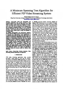
Figure 2.3 Percentage error in approximate average -diameter
2.2 Approximate Average-Diameter
We compared the average diameter in computer-generated random labeled-trees to the expected value computed using Szekeres' formula. The mean diameter was computed for randomly generated trees with up to one million nodes, and averaged for 100 different trees of each order.
The curve fitting result for the diameter means, obtained using a
least-square-fit program, was 3.33125n½, showing a difference of 0.010921n½ from
27
Szekeres' formula.
The curve fitting error, illustrated in Figure 2.3, stabilizes for
n ≥ 1100. To generate a random labeled-tree in linear time, we used a randomly generated Prüfer code [47].
Then, we examined three different approaches for calculating the
diameters of the trees. The first diameter-calculation algorithm takes a naïve approach by examining the paths between all pairs of leaves in the tree. Floyd algorithm, this approach takes O(n3 ) time.
Employing the Warshall-
The second approach repeatedly
removes all the leaves in the tree, until a single path remains. The diameter is equal to twice the number of deletions, plus the length of the remaining path. Using an efficient data structure, such as a queue, to maintain the order by which leaves are deleted, this approach takes linear time. The third approach, proposed by Handler [36], performs a depth-first search from an arbitrary node, u, in the tree to find the farthest node v from u. Node v will always be at one end of a longest path in the tree [84, 85]. Then, the algorithm performs a second depth-first search to find the farthest node z from v. The length of this path from v to z gives the diameter of the tree [36]. This method computes the diameter in linear time. To distinguish the speed of the two linear-time methods of computing diameter, we compared their execution times on a PC with a Pentium III / 500 MHz processor, using trees with 50 to one million nodes. The time taken by each algorithm was less than 3 milliseconds for n ≤ 1000. As the number of nodes increased, the leaf-deletion algorithm became clearly faster than Handler's algorithm.
28
Using a polynomial-fit program, we
determined that the execution time, in microseconds, taken by Handler's algorithm and the leaf-deletion algorithm was (2.79n – 43265) and (0.67n – 11716), respectively. The above three methods for computing tree-diameter may be used with unlabeled trees, where an arbitrary labeling of the nodes can be assigned before applying the algorithms.
A random unlabeled-tree can be generated in polynomial time using an
algorithm devised by Alonso et al. [11, 12].
29
CHAPTER 3 QUALITY OF AN APPROXIMATE DCMST
3.1 Polynomially-Solvable Cases
Four cases of the DCMST problem can be exactly solved in polynomial time. When the diameter constraint k = n – 1, an MST is the solution. When k = 2, the solution is a smallest-weight star, where a star is a tree with at most one non-leaf. Let DCMST(k) denote (an optimal) DCMST with diameter no more than k.
A DCMST(2) can be
computed in O(n2 ) time by comparing the weight of every n-node star in G.
A
DCMST(3) can be computed in O(n3 ) time by computing all spanning trees with diameter no more than 3 and choosing a spanning tree having the smallest weight as follows: Clearly, in a DCMST(3) of graph G, every node must be of degree 1 except at most two nodes, call them u and v. The edge (u, v) is the central edge of DCMST(3). To construct a spanning tree with diameter no more than 3, select an edge to be the central edge, (u, v). Then, for every node x in G, x ∉{u, v}, include in the spanning tree the smaller of the two edges (x, u) and (x, v). To obtain a DCMST(3), compute all such spanning trees — with every edge in G as the central edge of one spanning tree — and select the one with
30
the smallest weight. In a graph of m edges, we have to compute m different spanning trees.
Each of these trees requires (n − 2) comparisons to select (x, u) or (x, v).
Therefore, the total number of comparisons required to obtain a DCMST(3) is (n − 2)m. For the case when all edge-weights in G are equal, we can consider G unweighted, and the spanning tree with the smallest diameter is an optimal solution for any k ≥ 2, if and only if a solution exists. Finding such a solution is trivial for all unweighted graphs that contain an n-node star.
For graphs not containing a spanning star, a minimum-
diameter spanning tree can be constructed as follows [8, 41]: For every node v in G, construct a breadth-first spanning tree (BFST), Tv. The radius of Tv is the maximum path length from v to any node in Tv, and it can be computed by keeping track of the distance of every node u from v when u is added to Tv during the BFST construction, without increasing the time complexity.
All minimum-radius spanning trees will have diameter
2r or 2r – 1. A minimum-diameter spanning tree will be a BFST of minimum radius r that contains exactly one node with distance r from the root, if such a tree exists, or any minimum-radius spanning tree if such a tree does not exist.
Since each BFST is
computed in O(m) time, and there are n possible BFSTs, the time complexity of finding a minimum-diameter spanning tree is O(mn).
31
3.2 The Special-Case Algorithm for DCMST(4)
We developed a special-case algorithm to compute an approximate DCMST(4).
The
algorithm starts with an exact DCMST(3), then it replaces higher-weight edges with smaller-weight edges, allowing the diameter to increase to 4.
The refinement process
first arbitrarily selects one end-node, u, of the central edge, (u, v), of DCMST(3), to be the center of DCMST(4). Let W(a, b) denote the weight of an edge (a, b). For every node x adjacent to v, the algorithm attempts to obtain another tree of smaller weight by replacing edge (x, v) with an edge (x, y), where y is adjacent to u, and W(x, y) < W(x, v). Furthermore, for all nodes z adjacent to u, W(x, y) ≤ W(x, z). Figure 3.1 illustrates an example of this possible replacement. If no such edge exists, we keep edge (v, x) in the tree. We use the same method to compute a second approximate DCMST(4), with v as its center.
Finally, the algorithm certifies the DCMST(4) having the smaller weight as
the approximate solution. Suppose there are ρ leaves adjacent to u in DCMST(3). Then, there are (n − ρ − 2) leaves adjacent to v. Therefore, it is required to make 2ρ (n − ρ − 2)
(3.1)
comparisons to get an approximate DCMST(4). The probability that u is connected to ρ leaves is: 2 ñ(n − ñ − 2 ) n =3
∑ 2 ñ(n
− ñ − 2)
=
6 ñ(n − ñ − 2 ) . ( n − 1)( n − 2)( n − 3)
ρ =1
32
(3.2)
To find the expected value for ρ, treat Equation 3.2 as a continuous function, take its first derivative with respect to ρ, and then set the derivative equal to zero and solve for ρ. This gives the value: ρ = (n – 2)/2.
Substituting this value of ρ into Equation 3.1, it
shows that, employing our special-case algorithm, the expected number of comparisons required to obtain an approximate DCMST(4) from a DCMST(3) is (n2 – 8n – 12)/2.
y
x
u
v
Figure 3.1 One step in constructing an approximate DCMST(4) from DCMST(3)
To obtain a crude upper bound on the approximate DCMST(k) weight (where k is the diameter constraint), observe that DCMST(3) and DCMST(4) are feasible (but often grossly suboptimal) solutions of DCMST(k) for all k > 4.
Using the special-case
heuristic, we compute an approximate DCMST(4) and compare its weight with that of DCMST(3) to verify that the heuristic provides a tighter upper-bound for approximate DCMST(k). Let W(T) denote the weight of tree T. Then, clearly for any k ≥ 5, W(MST) ≤ W(DCMST(k)) ≤ W(DCMST(4)) ≤ W(DCMST(3)).
33
Since the exact DCMST for large graphs cannot be determined in a reasonable time, we use the upper bounds, along with the ratio of the weight of the approximate DCMST to the weight of the unconstrained MST, as a rough measure of the quality of the solution. We implemented the special-case heuristic for DCMST(4) sequentially on a PC with a Pentium III / 500 MHz processor. We also parallelized it and implemented it on the MasPar MP-1. We used complete graphs of orders between 50 and 3000, with randomly generated weights either ranging between 1 and 1000 or ranging between 1 and 10000. We also used complete graphs forced to have Hamiltonian-path MSTs with the same ranges of edge weights.
The sequential and parallel implementations produced similar
results for both random graphs and randomly generated graphs forced to have Hamiltonian-path MSTs. The change of the upper bound on edge weight did not have any noticeable effect, either.
The special-case heuristic for DCMST(4) produced
approximate solutions with weight roughly half that of exact DCMST(3), independent of n, as will be shown in Figures 8.1 and 8.2.
The time to refine a DCMST(3) into an
approximate DCMST(4) was about 1% of the time needed to calculate a DCMST(3), independent of n.
This heuristic is not suited for incomplete graphs since they are
unlikely to contain a spanning tree with diameter 3.
34
CHAPTER 4 THE IR1 ITERATIVE-REFINEMENT ALGORITHM Our three general iterative-refinement-strategy-algorithms first compute an unconstrained MST, and then iteratively refine this MST by edge-replacement until the diameter constraint is satisfied.
General iterative-refinement-algorithm IR1, which we present in
this chapter, iteratively penalizes the edges near the center of the MST by increasing their weight and then recomputes the MST. This attempts to lower the diameter by breaking up long paths from the middle, replacing them by shorter ones.
4.1 The Algorithm
The heart of Algorithm IR1 is a problem-specific penalty function. A penalty function succinctly encodes how many edges to penalize, which edges to penalize, and what the penalty amount must be, where the penalty is an increase in edge weight.
In each
iteration of IR1, as described in Algorithm 1, an MST of the graph with the current weights is computed, and then a subset of tree edges are penalized (using the penalty function), so that they are discouraged from appearing in the MST in the next iteration.
35
w1
w5
w3
w4 w2
w6
w1 < w2 < w3 < w4 < w5 < w6 (a)
(b)
(c)
(d)
(e) Figure 4.1 An example of cycling in IR1
Obviously, an edge at the center of a long path is a good candidate to be penalized, since
36
it would split each of the longest paths in the current tree into two subpaths of equal length.
However, penalizing only one edge per iteration may not be sufficient, as
illustrated by the example of Figure 4.1.
ALGORITHM 1 (IR1(G, k)). begin fails := 0; G’ := G; Tmin := MST of G; T := Tmin; while (((diameter of T) > k) and (fails ≤ 15)) do G’ := G’ with edges closest to the center of Tmin penalized; Tmin := MST of G’ ; /* computed using the new edge-weights */ if (((diameter of Tmin) < (diameter of T)) or (((diameter of Tmin) = (diameter of T)) and (W(Tmin) < W(T)))) then begin T := Tmin; fails := 0; end else fails := fails + 1; end while return T end.
For this complete graph and a specified diameter bound of 2, the MST is the path (w1 , w3 , w2 ), shown in Figure 4.1(b).
After penalizing the center edge, w3 , and
recomputing the MST, we get the path (w1 , w4 , w2 ), shown in Figure 4.1(c). The center edge w4 on this path is penalized next, producing the path in Figure 4.1(d). The algorithm fails to reduce the diameter of this tree as well, producing the tree in Figure 4.1(e), which, in the next iteration, regenerates the original MST.
37
The iterative refinement cycles
among these paths of diameter 3, and never finds any of the four spanning trees of diameter 2. However, if two edges are penalized in every iteration, there is no cycling for this example. The solution is found in three iterations, as shown in Figure 4.2. Such is the case for every edge-weighted graph with n = 4. But for n = 5, penalizing two edges per iteration may not be sufficient. To reduce the possibility of cycling, the number of edges to be penalized per iteration should increase with n. However, it must be kept in mind that penalizing too many edges may result in the solution being too far from optimal. This is because in the space of all nn
– 2
labeled spanning trees, the iterative refinement in such a case would jump (in a
single iteration) from one tree to another, which is many edges different, thereby missing a number of feasible solutions with perhaps smaller weight.
Therefore, the number of
edges penalized must be a slow-growing function of n, say log2 n.
All the edges
penalized should be close to the center of the current spanning tree where the center of a tree consists either of one node or one edge, depending on whether its diameter is even or odd. The edges to be penalized should be the ones incident to the center. If more edges are required to be penalized (when the degree of the center node is less than log2 n), then the edges at distance two from the center node should be chosen, and so on. A tie can be broken by choosing the higher-weight edge to penalize. Another issue to consider in designing a penalty function is the penalty amount. To be effective without causing overflow, the penalty value must relate to the range of the weights in the spanning tree.
Let W(l) denote the current weight of an edge l being
38
w1
w5 w4 w2
w6
w3
w1 < w2 < w3 < w4 < w5 < w6 (a)
(b)
(c)
(d) Figure 4.2 Finding an approximate DCMST(2) by penalizing 2 edges per iteration penalized, and wmax and wmin denote the largest and the smallest edge-weight,
39
respectively, in the current MST. Also, let distc(l) denote the distance of an edge l from the center node, plus one. When the center is a unique node, v c, all the edges l incident to v c have distc(l) = 1, the ones at distance one from v c have distc(l) = 2, and so on. When the center is an edge lc, it has distc(lc) = 1, an edge l incident to only one end-point of the center edge has distc(l) = 2, and so on. Therefore, the penalty amount imposed on the tree edge l is given by: (W ( l ) − wmin ) wmax MAX , ε , distc(l ) ( wmax − wmin ) where ε > 0 is a minimum mandatory penalty imposed on an edge, chosen to be penalized.
This minimum penalty ensures that the iterative refinement makes progress in
every iteration, and does not stay at the same spanning tree by imposing zero penalties to all the edges (in situations, for example, when all the penalized edges have weights equal to wmin ). In a typical implementation, in which weights are stored as integer values, the value of ε may be set to 1. Clearly, the penalty amount is proportional to the weight of the penalized edge and inverse-proportional to its distance from the center of the current MST.
The penalty
amount can be as high as wmax/distc(l), and it decreases as the penalized edge becomes farther away from the center of the tree. This was done because replacing an edge with a small distc(l) in the current tree can break a long path into two significantly shorter subpaths, rather than a short subpath and a long one. Also, an edge with a smaller weight is penalized by a smaller amount than one with a larger weight if they have the same
40
value of distc(.) to makes it less likely for the larger-weight edge to appear in the next MST.
4.2 Implementation
We parallelized Algorithm IR1 and implemented it on the MasPar MP-1. We ran the code for IR1 on random graphs with up to 3000 nodes, whose minimum spanning trees are forced to be Hamiltonian paths, and whose edge weights were randomly selected numbers between 1 and 1000. The tree weights resulting from IR1 are reported as factors of the unconstrained MST weight.
The average constrained spanning-tree weights with
diameter n/10 were 1.068, 1.036, and 1.024 for n = 1000, 2000, and 3000, respectively. This indicates remarkable performance of this iterative-refinement algorithm when the diameter constraint is a large fraction of the number of nodes. The algorithm was also fast, as it reduced the diameter of a 3000-node complete graph from 2999 to 103 in about 15 minutes.
Nonetheless, this iterative-refinement algorithm was not able to obtain
approximate DCMST(k) when k is a small fraction of the number of nodes, such as n/20. Thus, it should be used only for large values of k.
41
4.3 Convergence
One problem with the approach of Algorithm IR1 is that it recomputes the MST in every iteration, which sometimes reproduces trees that were already examined, even when the replacement increases the diameter.
Algorithm IR1 terminates when the current MST
diameter is no more than k, or when it cannot improve the current MST further. The latter case is identified by 15 consecutive iterations that reduce neither the diameter nor the weight of the current MST.
Our empirical study showed that allowing IR1 to
continue past 15 consecutive non-improving iterations did not result in better solutions when the edge weights ranged from 1 to 10000. When it was allowed to run for 500 iterations (regardless of non-improving iterations), Algorithm IR1 succeeded in finding a solution when the diameter constraint k ≥ n/10, but failed to find a DCMST when k was a small constant.
We present a different iterative-refinement algorithm in the next chapter
that avoids the cycling problem, and produces solutions with smaller values of k.
42
CHAPTER 5 THE IR2 ITERATIVE-REFINEMENT ALGORITHM The next iterative-refinement algorithm, IR2, does not recompute the MST in every iteration; rather, a new spanning tree is computed by modifying the previously computed one.
The modification performed does not regenerate previously generated trees and it
guarantees the algorithm will terminate. Unlike IR1, this algorithm removes one edge at a time and prevents cycling by moving away from the center of the spanning tree whenever cycling becomes imminent.
Figure 5.1 illustrates how this technique prevents
cycling for the original graph of Figure 4.1.
After computing the MST, the algorithm
considers the middle edge (shown in bold) as the candidate for removal, as in Figure 5.1(b). But this edge does not have a replacement that can reduce the diameter, so the algorithm considers edges a little farther away from the center of the tree.
The edge
shown in bold in Figure 5.1(c) is the highest-weight such edge. As seen in Figure 5.1(d), the algorithm is able to replace it by another edge, and that reduces the diameter. This algorithm guarantees that the diameter does not increase in any iteration and in fact can reduce the diameter to a small constant (less than 1% of the number of nodes in the graph). IR2 starts by computing the unconstrained MST for the input graph G = (V, E). Then, in each iteration, it removes one edge that breaks a longest path in the spanning tree and
43
replaces it by a non-tree edge without increasing the diameter.
The algorithm requires
computing eccentricity values for all nodes in the spanning tree in every iteration.
w1
w5
w3 w6
w4 w2
w1 < w2 < w3 < w4 < w5 < w6 (a)
(b)
(c)
(d)
Figure 5.1 An example of IR2
The initial MST can be computed using Prim's algorithm.
The initial eccentricity
values for all nodes in the MST can be computed using a preorder tree-traversal where each node visit consists of computing the distances from that node to all other nodes in This requires a total of O(n2 ) computations.
As the spanning tree
changes, we only recompute the eccentricity values that change.
After computing the
the spanning tree.
44
MST and the initial eccentricity values, the algorithm identifies one edge to remove from the tree and replaces it by another edge from G until the diameter constraint is met or the algorithm fails.
When implemented and executed on a variety of inputs, we found that
this process required no more than 3n iterations. Each iteration consists of two parts. In the first part, described in Section 5.1, we find an edge whose removal can contribute to reducing the diameter, and in the second part, described in Section 5.2, we find a good replacement edge.
The IR2 algorithm is shown in Algorithm 2, and its two different
edge-replacement subprocedures are shown in Algorithms 3 and 4. We use eccT(u) to denote the eccentricity of node u with respect to spanning tree T; the maximum distance from u to any other node in T.
The diameter of a spanning tree T is given by
MAX{eccT(u)} over all nodes u in T.
45
ALGORITHM 2 (IR2(G, T, k)). begin if (T is undefined) then T := MST of G; compute eccT (z) for all z in V; C := ∅; move := false; repeat diameter := MAX {ecc T ( z)} ;
/* G = (V, E) */
z∈V
if (C = ∅) then if (move = true) then begin move := false; C := edges (u, z) that are one edge farther from the center of T than in the previous iteration; end else C := edges (u, z) at the center of T; repeat (x, y) := highest weight edge in C; /* This splits T into two trees: subtree1 and subtree2 */ until ((C = ∅) or ( MAX {eccT (u )} = MAX { eccT ( z )} )); z ∈subtree 2
u∈subtree1
if (C = ∅) then /* no good edge to remove was found */ move := true; else begin remove (x, y) from T; get a replacement edge and add it to T; recompute eccT (z) for all z in V; end until ((diameter ≤ k) or (edges to be removed are farthest from center of T)); return T end.
46
5.1 Selecting Edges for Removal
To reduce the diameter, the edge removed must break a longest path in the tree and should be near the center of the tree. The center of spanning tree T can be found by identifying the nodes u in T with eccT(u) = diameter/2, the node (or two nodes) with minimum eccentricity. Since we may have more than one edge candidate for removal, we keep a sorted list of candidate edges.
This list, which we call C, is implemented as a max-heap sorted
according to edge weights, so that the highest-weight candidate edge is at the root. Removing an edge from a tree does not guarantee breaking all longest paths in the tree. The end nodes of a longest path in T have maximum eccentricity, which is equal to the diameter of T. Therefore, we must verify that removing an edge splits the tree T into two subtrees, subtree1 and subtree2, such that each of the two subtrees contains a node v with eccT(v) equal to the diameter of the tree T. If the highest-weight edge from heap C does not satisfy this condition, the algorithm removes it from C and considers the next highest.
This process continues until the algorithm either finds an edge that breaks a
longest path in T or the heap, C, becomes empty. If the algorithm goes through the entire heap, C, without finding an edge to remove, it must consider edges farther from the center. This is done by identifying the nodes u with eccT(u) = diameter/2 + bias, where bias is initialized to zero, and incremented by 1 every time the algorithm goes through C without finding an edge to remove. Then, the
47
algorithm recomputes C as all the edges incident to set of nodes u.
Every time the
algorithm succeeds in finding an edge to remove, bias is reset to zero. This method of examining edges helps prevent cycling since we consider a different edge every time until an edge that can be removed is found.
But to guarantee the
prevention of cycling, always select a replacement edge that reduces the el ngth of a path in T.
This will ensure that the refinement process will terminate, since it will either
reduce the diameter below the bound, k, or bias will become so large that the algorithm tries to remove the edges incident to the end-points of the longest paths in the tree. In the worst case, computing heap C examines many edges in T, thereby requiring O(n) comparisons. In addition, sorting C will take O(n log n) time. A replacement edge is found in O(n2 ) time since the algorithm must recompute eccentricity values for all nodes to find the replacement that helps reduce the diameter.
Therefore, the iterative
process, which removes and replaces edges for n iterations, will take O(n3 ) time in the worst case. Since heap C has to be sorted every time it is computed, the execution time can be reduced by a constant factor if we prevent C from becoming too large. This is achieved by an edge-replacement method that keeps the tree T fairly uniform so that it has a small number of edges near the center, as we will show in the next section. Since C is constructed from edges near the center of T, this will keep C small.
48
5.2 Selecting a Replacement Edge
When an edge is removed from a tree T, the tree T is split into two subtrees: subtree1 and subtree2.
Then, we select a non-tree edge to connect the two subtrees in a way that
reduces the length of at least one longest path in T without increasing the diameter. The diameter of T will be reduced when all longest paths have been so broken. We develop two methods, ERM1 and ERM2, to find such replacement edges.
5.2.1 Edge-Replacement Method ERM1
The first edge-replacement-method, shown in Algorithm 3, selects a minimum-weight edge (a, b) in G connecting a central node a in subtree1 to a central node b in subtree2. Among all edges that can connect subtree1 to subtree2, no other edge (c, z) will produce a tree such that the diameter of (subtree1 ∪ subtree2 ∪ {(c, z)}) is smaller than the diameter of (subtree1 ∪ subtree2 ∪ {(a, b)}). However, such an edge (a, b) is not guaranteed to exist in incomplete graphs.
49
ALGORITHM 3 (ERM1(G, T, subtree1, subtree2, move)). begin recompute eccsubtree1(.) and eccsubtree2(.) for all nodes in each subtree; m 1 := MIN {ecc subtree1 (u )} ; u∈subtree1
m 2 := MIN {ecc subtree 2 ( u )} ; u∈subtree 2
(a, b) := minimum-weight edge in G that has: (a ∈ subtree1) and (b ∈ subtree2) and (eccsubtree1(a) = m 1) and (eccsubtree2(b) = m 2); if (such an edge (a, b) is found) then add edge (a, b) to T; else begin add the removed edge (x, y) back to T; move := true; end if ((C = ∅) or (bias = 0)) then begin move = true; C = ∅; end return edge (a, b) end.
Since there can be at most two central nodes in each subtree, there are at most four edges to select from.
The central nodes in the subtrees can be found by computing
eccsubtree1 (.) and eccsubtree2 (.) in each subtree, then taking the nodes v with eccsubtree(v) = MIN{eccsubtree(u)} over all nodes u in the subtree that contains v. This selection can be done in O(n2 ) time. Finally, the boolean variable move is set to true every time an edge incident to the center of the tree is removed. This causes the removal of edges farther from the center of the tree in the next iteration of the algorithm, which prevents removing the recently added edge, (a, b).
50
This edge-replacement method seems fast at the first look, because it selects one out of four edges.
However, in the early iterations of the algorithm, this method creates
nodes of high degree near the center of the tree, which causes C to be very large. This, as we have shown in the previous section, causes the time complexity of the algorithm to increase by a constant factor.
Furthermore, having at most four edges from which to
select a replacement often causes the tree weight to increase significantly.
5.2.2 Edge-Replacement Method ERM2
The second edge-replacement-method, shown in Algorithm 4, computes eccsubtree1 (.) and eccsubtree2 (.) values for each subtree individually, as in ERM1. Then, the two subtrees are joined as follows. Let the removed edge (x, y) have x ∈ subtree1 and y ∈ subtree2. The replacement edge will be the smallest-weight edge (a, b) which (i) guarantees that the new edge does not increase the diameter, and (ii) guarantees reducing the length of a longest path in the tree at least by one. We enforce condition (i) by: eccsubtree1 (a) ≤ eccsubtree1 (x) AND eccsubtree2 (b) ≤ eccsubtree2 (y) , and condition (ii) by: eccsubtree1 (a) < eccsubtree1 (x) OR eccsubtree2 (b) < eccsubtree2 (y) . If no such edge (a, b) is found, we must remove an edge farther from the center of the tree, instead.
51
ALGORITHM 4 (ERM2(G, T, subtree1, subtree2, x, y, move)). begin recompute eccsubtree1(.) and eccsubtree2(.) for all nodes in each subtree; m 1 := eccsubtree1(x); m 2 := eccsubtree2(y); (a, b) := minimum-weight edge in G that has: (a ∈ subtree1) and (b ∈ subtree2) and (eccsubtree1(a) ≤ m 1) and (eccsubtree2(b) ≤ m 2) and ((eccsubtree1(a) < m 1 or (eccsubtree2(b) < m 2)); if (such an edge (a, b) is found) then add edge (a, b) to T; else begin add the removed edge (x, y) back to T; move := true; end return edge (a, b) end.
Since ERM2 is not restricted to the centers of the two subtrees, it works better than ERM1 on incomplete graphs. In addition, it can produce DCMSTs with smaller weights because it selects a replacement from a large set of edges, instead of 4 or fewer edges as in ERM1. The larger number of edges increases the total time complexity of IR2 with ERM2 by a constant factor over IR2 with ERM1. However, this method does not create nodes of high degree near the center of the tree as in ERM1. This helps keep the size of heap C small in the early iterations, reducing the time complexity of IR2 by a constant factor.
52
(Spanning Tree Weight) / (MST Weight)
21 19 17 15
DCMST(3)
13
Special-Case Approx. DCMST(4)
11 9
IR2-ERM1: Approx. DCMST(10)
7
IR2-ERM2: Approx. DCMST(10)
5 3 1 100
200
300
400
500
1000
Number of Nodes (n )
Figure 5.2 Weight quality of approximate solution, in randomly weighted complete-graphs with Hamiltonian-path MSTs, produced by IR2 using two different edge-replacement methods
5.3 Implementation
First, we parallelized Algorithm IR2 and implemented it on the MasPar MP-1, using complete random-graphs and complete graphs forced to have Hamiltonian-path MSTs, where edge weights were randomly selected integers between 1 and 1000.
We also
implemented IR2 sequentially on a PC with a Pentium III / 500 MHz processor using random-graphs and graphs forced to have Hamiltonian-path MSTs, where edge weights
53
were randomly selected integers between 1 and 10000, and the graph densities ranged from 20% to 100%. All input graphs had orders ranging from 50 to 2000, where 20 different graphs were generated for each order, density, and type of graphs. As expected, IR2 did not enter an infinite loop, and it always terminated within 3n iterations. The weight quality of approximate DCMST(10) successfully obtained by this iterative-refinement algorithm using the two different edge replacement methods, ERM1 and ERM2, for graphs with Hamiltonian-path MSTs is shown in Figure 5.2. The diagram shows the weight of the computed approximate DCMST as a multiple of the weight of the unconstrained MST. It is clear that IR2 produced approximate solutions lower than the upper bounds, and IR2 using ERM2 produced lower weight solutions than IR2 using ERM1.
As expected, the time required by IR2 using ERM1 to obtain approximate
DCMSTs was greater than the time required by IR2 using ERM2. In addition, ERM1 required more memory space than ERM2, because the size of C when we use ERM1 is significantly larger than its size when ERM2 is used. This is caused by the creation of high-degree nodes by ERM1, as explained in Section 5.2.
For the remainder of this
dissertation, we will discuss the behavior of Algorithm IR2 only using ERM2 as the edge-replacement method. When IR2 (using ERM2) was tested on random complete-graphs, the weight quality of approximate DCMST(10) produced by IR2 exceeded the weight of approximate DCMST(4) produced by the special-case algorithm when the edge weights were randomly selected integers between 1 and 1000, but not when the range of edge weights was 1 to 10000.
In the latter case, IR2 also produced approximate DCMST(5) with
54
weight lower than the approximate DCMST(4) produced by the special-case algorithm. No spanning tree of diameter 3 was found in our samples of sparse graphs, and therefore, the special-case heuristic did not obtain any spanning trees of diameter 4 in those graphs. The average time required to produce approximate solutions with n = 2000 for DCMST(5) and DCMST(10), respectively,
was 1924 and 1296 seconds in random
complete-graphs, and 1231 and 538 seconds in random graphs with 20% density. The average weight of solutions with n = 2000 for DCMST(5) and DCMST(10), respectively, as a factor of the unconstrained MST weight, was 159 and 48 in random complete-graphs and 29 and 10.8 in random graphs with 20% density.
In random graphs of all tested
densities, the weight of solutions, as a factor of the unconstrained-MST weight, increased with n. In graphs with Hamiltonian-path MSTs, the weight of approximate DCMST(10) produced by IR2 (using ERM2) was lower than the weight of approximate DCMST(4) produced by the special-case algorithm, regardless of the range of edge weights.
The
upper bounds (trees of diameter 3 and 4) were not available for sparse graphs of this type, either.
The average time required by IR2 to produce approximate solutions, in graphs
with Hamiltonian MSTs, with n = 2000 for DCMST(5) and DCMST(10), respectively, was 1488 and 1038 seconds in random complete-graphs, and 3038 and 1053 seconds in random graphs with 20% density.
The average weight of solutions as a factor of the
unconstrained MST weight, was approximately 26 and 9 for DCMST(5) and DCMST(10), respectively, in random complete-graphs, independent of n.
In random
graphs with 20% density, the weight of solution, as a factor of the unconstrained MST
55
weight, decreased with n. The weights of DCMST(5) and DCMST(10), respectively, as a factor of MST weight, was 44.6 and 18.9 for n = 50 and 21.5 and 11.1 for n = 2000. The weight of solutions, as a factor of MST weight, in our samples of graphs with Hamiltonian-path MSTs did not increase with n because of the way these graphs were generated. To force a randomly generated graph to have a Hamiltonian-path MST, we randomly selected edges to include in the Hamiltonian path and randomly assigned them integer weights between 1 and 100.
The rest of the edges were randomly generated
integer-weights between 101 and 10000. Therefore, the average weight of an MST-edge is 50, and the average weight of a non-MST edge is 5050. However, there are only (n – 1) edges in the MST and there are O(n2 ) non-tree edges in the rest of the graph. Thus, as n increases, the ratio: (average weight of a non-MST edge) / (average weight of an MST edge) decreases.
This effect becomes clearer as the number of edges exceeds 10000.
Consequently, we evaluate the solutions' weights in this type of graphs based on the upper and lower bounds (whenever available) calculated for the same set of graphs. However, the time taken by the algorithm can be compared with other types of graphs, where it can be seen that IR2 requires a longer time to obtain a solution when the diameter of the unconstrained MST is larger. With all input graphs used for IR2, the weights of solutions and time required to obtain them increased whenever the diameter bound, k, was decreased. The quality of IR2 will be discussed further, in Chapter 8, when it is compared to the other algorithms we developed for the DCMST problem.
56
5.4 Convergence
As was shown in Sections 5.2 and 5.3, Algorithm IR2 is guaranteed to terminate, but it is not guaranteed to produce a solution. The failure rate of IR2 does not depend on what fraction of n the value of the bound on diameter, k, is. Rather, it depends on how small the constant, k, is. To see this, we must take a close look at the way we move away from the center of the tree while selecting edges for removal. Note that the algorithm will fail only when it tries to remove edges incident to the end-points of the longest paths in the spanning tree. Also note that the algorithm moves away from the center of the spanning tree every time it goes through the entire set C without finding a good replacement edge, and it returns to the center of the spanning tree every time it succeeds. Thus, the only way the algorithm fails is when it is unable to find a good replacement edge in diameter/2 consecutive attempts, each of which includes going through a different set of C.
Empirical results show that it is unlikely that the algorithm will fail for 8
consecutive times, which makes it suitable for finding an approximate DCMST when the value of k is a constant greater than or equal to 15. When the input graphs were forced to have Hamiltonian-path MSTs, Algorithm IR2 was unable to find a spanning tree with diameter no more than 10 in some cases.
In
graphs with 100 ≤ n ≤ 2500, our empirical results show a failure rate of 10% for k = 10 and 15% for k = 5. The success rate of IR2 (using ERM2) with (unrestricted) random complete-graphs was 90% for n ≥ 200. In all graphs, the times required by IR2 to obtain a solution increased when the value of k was decreased. 57
When tested on incomplete graphs, Algorithm IR2 (using ERM2) was more than 65% successful in obtaining an approximate DCMST(5) for random graphs and graphs with Hamiltonian-path MSTs, where the density was at least 20% and n ≥ 500. The success rate dropped slowly as the density of the input graph was decreased. For the same types of graphs and the same densities, the success rate also dropped when n was reduced below 500, where Algorithm IR2 becomes only 30% successful in finding an approximate DCMST(5) in graphs with n = 50 and density = 20%.
This is
understandable since the number of edges grows faster than the number of nodes. For example, when density is 20%, there are 24950 edges in a graph of 500 nodes, but only 245 edges in a graph of 50 nodes. We measured and analyzed the time taken by IR2 to terminate. We measured the time taken by IR2 (using ERM2) to terminate successfully on the Pentium III / 500 MHz machine, and we obtained the following equations using a polynomial-fit program. When using complete random-graphs, IR2 required (0.111n3 + 62.7n2 – 29583.7n + 2170981) and (0.0736n3 – 21.5n2 + 10100n – 1230000) microseconds for k = 5 and k = 10, respectively.
For random graphs with 20% density, IR2 required (0.191n3 +
77.2n2 – 42250.8n + 3152147) and (0.0639n3 +9.55 n2 – 5573.5n – 342626) microseconds for k = 5 and k = 10, respectively. This shows that the time required by IR2 for this type of graphs is almost unaffected by the change in graph density. When using complete graphs with Hamiltonian-path MSTs, IR2 required (0.187n3 + 50.2n2 – 28288.1n + 2119730) and (0.121n3 + 22n2 – 11709.6n + 74699121) microseconds for k = 5 and k = 10, respectively.
For graphs with Hamiltonian-path MSTs and 20%
58
density, IR2 required (0.248n3 + 38.4n2 – 26746.2n + 2120446) and (0.181n3 – 133.8n2 + 71780.63n – 7707461) microseconds for k = 5 and k = 10, respectively. This shows that, in this type of graphs, the time required by IR2 increases slightly when the graph density is reduced.
59
CHAPTER 6 THE CIR ITERATIVE-REFINEMENT ALGORITHM The composite-iterative-refinement algorithm, CIR, first computes an unconstrained MST, then if the MST does not satisfy the constraint, iteratively refines this MST by edge replacements until the diameter constraint is satisfied or the algorithm fails.
Algorithm
CIR consists of two stages: Algorithms IR1 and IR2, described in Chapters 4 and 5. The first stage, Algorithm IR1, is fast, but it normally cannot reduce the diameter to the given bound, k.
It terminates when it is unable to improve the current spanning tree for 15
consecutive iterations.
The second stage, Algorithm IR2, refines the spanning tree
further, until a solution is found or the algorithm fails. The only difference in our use of IR2 in this chapter is that it takes the spanning tree produced by IR1 as input, instead of starting with an unconstrained MST as in Chapter 5.
6.1 Implementation
Algorithm CIR was implemented sequentially on a PC with a Pentium III /500 MHz processor using graphs of orders 50 to 3000 and densities from 20% to 100%. Twenty different random graphs and twenty different graphs with Hamiltonian-path MSTs were
60
randomly generated for each order and density.
CIR always terminated after no more
than 3n iterations of IR2. It was successful in more than 80% obtaining an approximate solution in complete graphs, including the cases when n = 3000 and k = 5, where the weight ratio (approximate DCMST to MST) was 251 for random graphs and 27 for graphs with Hamiltonian-path MSTs.
The weights of solutions produced by CIR were
lower than the upper bounds in complete graphs.
IR1 terminated after reducing the
diameter by about 20%, producing a spanning tree with weight approximately 1.05 times MST weight. When the density of the graphs was gradually reduced to 20%, the success rate of CIR remained above 60%, but the weights of solutions deteriorated quickly. Overall, the time taken by IR1 was about 1% of the total CIR time. The time taken by CIR, in seconds, to obtain an approximate DCMST(5) in randomly-generated completegraphs was 245, 815, and 1924 for n = 1000, 1500, and 2000, respectively. Using graphs with Hamiltonian-path MSTs as input, the weights of solutions, as compared to the upper and lower bounds, had the same quality as in random graphs, with the same success rate. However, using graphs with Hamiltonian-path MSTs, CIR obtained an approximate DCMST(5) in 292, 1130, and 3300 seconds for n = 1000, 1500, and 2000, respectively. For all graphs, the weights of solutions, and the time required by CIR to obtain them, increased whenever k was reduced or whenever n was increased.
61
6.2 Convergence
The first phase of Algorithm CIR, which is IR1, is guaranteed to terminate because it will either reduce the diameter below the given bound, or it will stop after failing to improve the solution for 15 consecutive iterations. Empirical evidence shows that allowing IR1 to continue past 15 consecutive unsuccessful-iterations does not result in noticeably lowerweight solutions for the DCMST problem by CIR. The second phase of CIR, which is IR2, is guaranteed to terminate (successfully or unsuccessfully), as shown in Chapter 5. Consequently, CIR will always terminate. Empirical results show that the success rate of CIR is slightly lower than the success rate of IR2 (without IR1). Algorithm IR1 is faster than Algorithm IR2. However, the time required by CIR is longer than the time required when IR2 is run using an unconstrained MST as input. In the first stage of CIR, the MST is recomputed by IR1, producing a spanning tree with a smaller diameter. This spanning tree, however, contains O(log n) edges that are not in the unconstrained MST. Furthermore, these edges are close to the center of the spanning tree produced by IR1. In the second stage of CIR, some of these O(log n) edges are replaced by IR2, which also replaces other edges and reduces the diameter further. If the edge replacements in the first stage of CIR are not very carefully selected, they may cause the second stage to require more iterations, and possibly decrease the weight-quality of the final solution. The time taken by CIR was measured on a PC with a Pentium III / 500 MHz processor. The input graphs had 50 to 3000 nodes, and densities ranging from 20% to
62
100%.
The edge weights were randomly-selected integers between 1 and 10000.
A
polynomial-fit program was used to obtain the following equations for the time taken by CIR to obtain an approximate solution.
When using random graphs as input, the time
required by CIR to compute approximate DCMST(5) and DCMST(10), respectively, was (0.236n3 + 9.92n2 – 2430.3n – 1050113) and (0.169n3 – 16.2n2 + 4941.7n – 402038) microseconds for complete graphs, and (0.278n3 + 74.1n2 – 42266.8n + 3030118) and (0.151n3 + 23.5n2 – 16146.5n – 1194858) microseconds for graphs with 20% density. This shows that the time required by CIR, for this type of graphs, is almost unaffected by the change in graph density.
Using graphs with Hamiltonian-path MSTs, the time
required by CIR to compute approximate DCMST(5) and DCMST(10), respectively, was (0.461n3 – 239.4n2 + 75896.98n – 3266577) and (0.233n3 – 30.5n2 + 13153.98n – 1039968) microseconds for complete graphs, and (0.394n3 – 1.11n2 + 203.51n + 704228) and (0.171n3 + 103.12n2 – 50536.3n + 4291839) microseconds for graphs with 20% density.
This shows that an increase in graph density in this type of graphs causes an
increase the time required by CIR to obtain a solution.
63
CHAPTER 7 THE ONE-TIME-TREE-CONSTRUCTION ALGORITHM In the one-time tree-construction strategy, a modification of Prim's algorithm is used to compute an approximate DCMST in one pass. Prim's original algorithm is chosen since it has been experimentally shown to be the fastest algorithm for computing an MST for large dense-graphs [57].
In addition, Prim's algorithm keeps the partially-formed tree
connected in every iteration of the MST-construction process.
This makes it easier to
keep track of the diameter, as opposed to keeping track of the diameters of the trees of a forest in Kruskal's algorithm.
Furthermore, using Kruskal's algorithm, a greedy strategy
will not be able to construct a spanning tree of diameter k in one pass if an intermediate step creates two non-spanning trees of diameter k/2. That makes it necessary to keep more information about the forest while the spanning tree is being constructed, and it may be necessary to do backtracking in some cases.
7.1 The Algorithm
The one-time-tree-construction algorithm, OTTC, starts with an arbitrary node, and grows a spanning tree by connecting the nearest neighbor that does not violate the
64
diameter constraint.
Algorithm OTTC is described in Algorithm 4, where we maintain
the following information for each node, u: near(u)
is a tree node candidate to be incident to u in the approximate DCMST.
W(u, v)
is the weight of edge (u, v).
dist(u, v)
is the (unweighted) distance from u to v if u and v are in the current tree, and is set to –1 if u or v is not in the tree.
ecc(u)
is the eccentricity of node u (the distance in the tree from u to the farthest node) if u is in the current tree, and is set to –1 if u is not in the tree.
To select near(u), we determine the edges that connect u to partially-formed tree, T, without increasing the diameter (as the first criterion) and among all such edges we want the one with minimum weight. In Segment 1 of Algorithm OTTC (described in Algorithm 4), the dist(.) and ecc(.) values for node z are set by copying from its parent node near(z). In Segment 2, the values of dist(.) and ecc(.) for the parent node are updated in n steps. In Segment 3, the values of dist(.) and ecc(.) are update for other nodes. We make use of the dist(.) and ecc(.) arrays, as described above, to simplify the OTTC computation.
65
ALGORITHM 4 (OTTC(G, k, z0)). begin VT := {z0}; ET := ∅; near(u) := z0 , for every u ∉ VT ; find a node z such that: W(z, near(z)) = MIN {W ( u, near (u ))} ; u ∈VT
while (|ET| < (n – 1)) do select the node z with the smallest value of W(z, near(z)); VT := VT ∪ {z}; ET := ET ∪ {(z, near(z))}; /* 1. set dist(z, u) and ecc(z) */ for u = 1 to n do if (dist(near(z), u) > –1) then dist(z, u) := dist(near(z), u) + 1; end for dist(z, z) := 0; ecc(z) := ecc(near(z)) + 1; /* 2. update dist(near(z), u) and ecc(near(z)) */ dist(near(z), z) := 1; if (ecc(near(z)) < 1) then ecc(near(z)) := 1; /* 3. update other nodes' values of dist(.) and ecc(.) */ for each tree node u other than z or near(z) do dist(u, z) := dist(u, near(z)) + 1; ecc(u) := MAX{ecc(u), dist(u, z)}; end for /* 4. update the near(.) values for other nodes in G */ for each node u not in the tree do if ((ecc(near(u)) + 1) > k) then examine all nodes in T to determine near(u); else compare W(u, near(u)) to W(u, z); end for end while return T end.
66
/* T = (VT, ET) */
In Segment 4, we update the near(.) values for every node not yet in the tree. If adding node z to the tree would increase the diameter beyond the constraint, we must reexamine all nodes of the tree to find a new value for near(z). This can be achieved by examining ecc(u) for nodes u in the tree; i.e., we need not recompute the tree diameter. This computation includes adding a new node, z, to the tree, where W(z, near(z)) is minimum, and the addition does not increase the tree diameter beyond the constraint. The time complexity of Segment 4 is O(n2 ) since it requires examining each node in the tree once for each non-tree node.
The while loop requires (n – 1) iterations. Each
iteration requires at most O(n2 ) steps, which makes the worst-case time-complexity of the algorithm O(n3 ). When G is incomplete, this algorithm does not always find an existing solution. Furthermore, the algorithm is sensitive to the node chosen for starting the spanning tree. Therefore, we compute n such trees, one for each starting node.
Then, we select the
spanning tree with the smallest weight. To reduce the time needed to compute a DCMST further, we select q starting nodes (q is independent of n) for OTTC at random, or we select the q nodes with the smallest sum of weights of the edges incident to each node. Now, producing q spanning trees, instead of n, reduces the overall time complexity by a factor O(n) when q is a constant. For incomplete graphs, we can choose the q nodes with the highest degrees, and break a tie by choosing the node with the smaller sum of weights of edges incident to it.
67
7.2 Implementation
We implemented Algorithm OTTC on a PC with a Pentium III / 500 MHz processor for graphs of up to 2000 nodes and densities ranging from 20% to 100%, where 20 random graphs and 20 graphs with Hamiltoniam-path MSTs were generated for each order and density. The edge weights were randomly-selected integers between 1 and 10000. We also parallelized OTTC and implemented it on the MasPar MP-1 for complete randomgraphs and graphs with Hamiltonian-path MSTs, where edge weights were randomlyselected integers between 1 and 1000.
The parallel and sequential implementations
produced similar results in terms of the performance of OTTC. The time required by OTTC to obtain an approximate DCMST using n start nodes was significantly larger than the time required by the other four algorithms presented in this dissertation.
We addressed this issue by running the algorithm for a carefully
selected small set of start nodes. We examined three different methods for choosing the set of start nodes. One node-selection-method, NSM1, selects the center nodes of the q smallest stars in G as start nodes. The second method, NSM2, selects q nodes from G at random. The third method, NSM3, is specific to incomplete graphs, and it selects the q nodes with the highest degrees in G, and breaks a tie by choosing the node with the smaller sum of weights of edges incident to it. We report the results using q = 20, where other small values for q (between 1 and 50) produced similar results.
The quality of
solution improved slowly with q, and the success rate of OTTC in obtaining a solution in incomplete graphs increased slowly with q.
68
Algorithm OTTC was always successful in obtaining a solution for complete graphs, including when k = 4. However, the success rate of OTTC declined as the density of input graphs was reduced, especially when using less than n start nodes. Here, we report the results (approximate solutions) for complete random-graphs.
When using n start
nodes, Algorithm OTTC required 600, 2154, and 5130 seconds to compute an approximate DCMST(5) with n = 1000, 1500, and 2000. OTTC using NSM1 produced approximate solutions for DCMST(5) in 29, 91, and 206 seconds with n = 1000, 1500, and 2000, respectively. OTTC using NSM2 produced approximate solutions with weight almost identical to those obtained using NSM1, but it took 6, 14, and 26 seconds to compute an approximate DCMST(5) with n = 1000, 1500, and 2000, respectively. The weights of approximate solutions obtained using n start nodes was better than using 20 start nodes by more than two times the weight of MST, but it took about n/20 times longer to run to completion.
This confirms the theoretical analysis that predicted an
improvement of O(n) in execution time over the n-iteration algorithm. The time required by OTTC grew slowly with k. For example, using OTTC with NSM2 to compute an approximate DCMST(150) required only ½ second longer than the time required to compute an approximate DCMST(4) for the same set of graphs with n = 1500. There was no difference in the weight quality (compared to the upper and lower bounds), or in the actual running time, when graphs with Hamiltonian-path MSTs were used as input for OTTC. In incomplete graphs, OTTC with NSM2 required the same time it did with complete graphs.
Using OTTC with NSM3 instead of NSM1 required a small amount of extra
69
time, but it had no noticeable effect on the weights of solutions or the success rate of the algorithm. Overall, the time required by OTTC was not affected by the change in graph density and whether or not the graph had a Hamiltonian-path MST.
7.3 Convergence
Algorithm OTTC starts with an arbitrary node, and grows a spanning tree by adding a node via the smallest-weight edge that does not violate the diameter constraint. When adding an edge would violate the diameter constraint, an alternative edge, which does not violate the diameter constraint, must be found. Since such an edge is guaranteed to exist in a complete graph, OTTC will always converge in complete graphs.
However, in
incomplete graphs, the algorithm is likely to fail as the density of the graph is reduced. As expected, empirical results show OTTC was always successful in obtaining an approximate solution in all types of complete graphs. When the density was reduced to 50%, it was necessary to run OTTC an average of 1.25 times for n = 100 and an average of 7.3 times for n = 1500, each time with a different arbitrary node, before an approximate DCMST(10) was found.
In graphs with 20% density, it was necessary to
run OTTC approximately 29 times for n = 100 and approximately 67 times for n = 1500, each time with a different arbitrary node, before an approximate DCMST(10) was found. The number of attempts required to obtain a solution increased with n, but it was always possible for OTTC to obtain an approximate solution for DCMST(10) within n attempts
70
in graphs with density of at least 20%.
However, OTTC, using n source nodes, was
unable to find a spanning tree with diameter 5 in sparse graphs when at least one existed, and its success rate in dense graphs was less than 100% for k = 5. The time required by OTTC was not affected by the change in graph density, where NSM2 required the same time as in complete graphs, and NSM3 required approximately the same time as NSM1. The success rate of NSM2 and NSM3, in obtaining a solution, was approximately the same. We used a polynomial-fit program to determine the equation for the time taken by OTTC on a PC with a Pentium III / 500 MHz processor. The time taken by OTTC using one source node was approximately (0.00299n3 + 0.33n2 – 28.4n + 1667) microseconds.
71
CHAPTER 8 PERFORMANCE COMPARISONS In this chapter, we present empirical results by implementing the iterative refinement and one-time-tree-construction algorithms on a Pentium III / 500 MHz processor, and we compare the performance of these algorithms based on the weight of approximate solutions obtained, required time, convergence and success rate, and the effects of different types of input. Graphs of different orders and densities, represented by their (n × n) weight matrices, were used as input.
The input graphs had 50 ≤ n ≤ 3000, where edge weights were
randomly generated integers, 1 to 10000.
Twenty different graphs were generated for
each order and density, and the mean values were calculated.
In addition, we used
randomly generated graphs with Hamiltonian-path MSTs, i.e., graphs whose MSTs are forced to have diameter (n − 1).
72
Weight Ratio
500
DCMST(3)
450
Special-Case Approx. DCMST(4)
400
CIR Approx. DCMST(5)
350
IR2-ERM2 Approx. DCMST(5) OTTC-NSM2 Approx. DCMST(5)
300 250 200 150 100 50 0 50
100
200
300
400
500
1000
1500
2000
Number of Nodes (n )
Figure 8.1 The ratio ((spanning-tree weight) / (MST weight)) in randomly weighted complete-graphs
Among all four general-algorithms we presented, only OTTC was always successful in obtaining an approximate solution for the DCMST problem in complete graphs regardless of the value of the diameter bound, k. However, the success rate of OTTC (using one source node) diminished quickly when the density of the graphs was reduced, especially with small values of the diameter bound, such as k = 5. Algorithms IR2 and CIR were not always successful in obtaining an approximate solution, but their success rate remained above 60%, even for graphs with 20% density and diameter constraint k = 5.
When OTTC was run using n start nodes, it was successful in obtaining an
approximate DCMST(10) in all graphs we tested, regardless of their density. However, OTTC using n start nodes was unable to obtain an approximate DCMST(5) in any graph
73
with 20% density, and it was unsuccessful in obtaining an approximate DCMST(5) in graphs with 50% density and n ≥ 1000, where algorithms IR2 and CIR verified that such solutions existed.
Algorithm IR1 was always successful in obtaining an approximate
solution in complete graphs when the diameter bound, k, was not less than n/10, but it was unsuccessful in obtaining a solution when k was a small constant, or when the graph was not dense. DCMST(3)
70
Special-Case Approx. DCMST(4) CIR Approx. DCMST(5) IR2-ERM2 Approx. DCMST(5)
60
OTTC-NSM2 Approx. DCMST(5)
Weight Ratio
50
40
30
20
10
0 50
100
200
300 400 500 Number of Nodes (n )
1000
1500
2000
Figure 8.2 The ratio ((spanning-tree weight) / (MST weight)) in randomly weighted complete-graphs with Hamiltonian-path MSTs
The special-case algorithm for DCMST(4) was always successful in finding an approximate solution in a graph that contains a spanning tree of diameter 3, and it was unsuccessful otherwise.
This special-case algorithm provided an upper bound on the
weights of approximate solutions produced by the general algorithms.
74
10 CIR Approx. DCMST(10)
9
IR2-ERM2 Approx. DCMST(10)
8
OTTC-NSM2 Approx. DCMST(10)
Weight Ratio
7 6 5 4 3 2 1 0 50
100
200
300 400 Number of Nodes (n )
500
1000
1500
Figure 8.3 The ratio((spanning-tree weight) / (MST weight)) in randomly weighted graphs with 20% density As seen in Figures 8.1, 8.2, and 8.3, Algorithm OTTC provided the lowest-weight solutions, regardless of the density of the graph, and whether or not it has a Hamiltonianpath MST.
Algorithm CIR produced approximate solutions with weight similar to the
weight of approximate solutions produced by IR2, and lower than the weight of the approximate DCMST(4) produced by the special-case algorithm.
Among all five
algorithms we presented for the DCMST problem, only IR2 and CIR could produce approximate solutions for values of k as small as 5 in sparse graphs. The time required by IR1, IR2, and CIR increased when k was reduced. The time required by OTTC increased slightly when k was increased.
However, OTTC (using
NSM2) was the fastest of the four general algorithms in obtaining an approximate solution.
Furthermore, it was the only general algorithm that did not require more time
75
6000 OTTC with n source nodes CIR
5000
IR2-ERM2
Time (seconds)
OTTC-NSM2
4000 3000 2000 1000 0 100
200
300
400
500
1000
1500
2000
Number of Nodes (n )
Figure 8.4 The time required by different algorithms to obtain an approximate DCMST(5) in randomly weighted complete-graphs
when the diameter of the unrestricted MST was increased. Figure 8.4 illustrates the time required by IR2, CIR, and OTTC to compute an approximate DCMST(5) in the same set of complete graphs. As the number of nodes increased, OTTC using NSM2 required less time than the other algorithms illustrated in the figure, but OTTC using n start nodes required more time than the other algorithms illustrated in this figure.
These results are
reflected by the coefficient of n3 in the equation of time required by OTTC, given in Chapter 7, which is lower than the coefficients of n3 in the equations of time required by other algorithms, given in earlier chapters. When OTTC was run with n source nodes, its required time was multiplied by n. The equations for the time required by OTTC and IR2, to obtain a DCMST(5) in randomly weighted complete-graphs, can be used to show that OTTC run with n source nodes requires more time than IR2 for graphs with n ≥ 81.
76
CHAPTER 9 CONCLUSION The DCMST problem has various practical applications, such as in distributed mutualexclusion, bit-compression for information retrieval, and linear lightwave networks.
We
presented a survey of the literature on the DCMST problem and presented new efficient approximate-algorithms that solve it.
We presented a study of the behavior of MST-
diameter in randomly generated graphs. algorithms for the DCMST problem.
Then, we developed five approximate The special-case algorithm for DCMST(4)
constructs an approximate DCMST(4) from an exact DCMST(3), and it is used in providing an upper bound on the weight of approximate solutions in dense graphs. When the diameter constraint is a large fraction of n, Algorithm IR1 uses the iterativerefinement strategy to provide high-quality solutions in a short amount of time. It starts with an unconstrained MST, and then it iteratively increases the weight of (log n) edges near the center of the MST and recomputes the MST. Algorithm IR2 uses the iterativerefinement strategy with more careful edge-replacements, and without recomputing the MST, to provide feasible solutions when k is a small constant. It serves as a tighter upper bound for other general algorithms for the DCMST problem, and it is the algorithm of choice for sparse graphs.
The composite-iterative-refinement algorithm, CIR, combines
IR1 and IR2, providing insight into their behavior.
77
Algorithm OTTC, which grows a
spanning tree of the desired diameter, was always successful in obtaining an approximate solution in complete graphs, and the solution was always lower than all upper bounds, even when using a small number of start nodes.
When OTTC was used with a small
number of start nodes, it was also the fastest of the four general algorithms we presented for solving the DCMST problem.
Consequently, OTTC is an excellent algorithm for
providing solutions for the DCMST problem, except in sparse graphs, where its success rate was significantly lower than that of IR2.
78
APPENDIX A PROGRAM CODE FOR COMPUTING EXACT AVERAGEDIAMETER
79
/******************************************************************************************** * Calculation of exact average-diameter for a tree of order n using Riordan's * equations for computing the number of trees with a given diameter. * ********************************************************************************************/ #include #include #include #include #include #include "gmp.h" /* this multi-precision library is available free from GNU */ #define maxn 52 #define MY_SEC (((after.ru_utime.tv_sec*1000000+after.ru_utime.tv_usec) \ -(before.ru_utime.tv_sec*1000000+before.ru_utime.tv_usec))/1000000.0) struct rusage before, after; long hsec, husec; long int who=RUSAGE_SELF; int S[maxn/2]; mpz_t power[maxn-2][maxn-4]; /* mpz_t is an arbitrarily-long integer */ mpz_t Factorial[maxn-1]; mpq_t G[maxn/2][maxn-1]; /* mpq_t is an arbitrarily-long rational number */ mpq_t D[maxn-1][maxn-1]; void Exponent(mpz_t *ans, int base, int expo) /*~~~~~~~~~~~~~~~~~~~~~~~~~~~~~~~~~~~~~~~~~~~~~~~~~~~~~~~~~~~~~~~~~~~~~~~*/ { if (expo < 0) mpz_set_ui(*ans,0); /* unacceptable exponents */ else if (expo == 1) mpz_set_ui(*ans,(unsigned long)base); else if (expo == 0 || base == 1) mpz_set_ui(*ans,1); /* includes 0^0: The Curious Identity */ else if (base == 0) mpz_set_ui(*ans,0); else mpz_set(*ans,power[base-2][expo-2]); } void AllPowers(int n_hi) /*~~~~~~~~~~~~~~~~~~~~~~~~~~~~~~~~~~~~~~~~~~~~~~~~~~~~~~~~~~~~~~~~~~~~~~~*/ /* power[i][j] contains (i+2)^(j+2) which means power[0][0] contains 2^2 */ /*~~~~~~~~~~~~~~~~~~~~~~~~~~~~~~~~~~~~~~~~~~~~~~~~~~~~~~~~~~~~~~~~~~~~~~~*/ { int base, expo; for (base = 2; base = max) max = abs(list[i]); return(max); } void FindMaxEccInSub(short *max1, short *max2) /*~~~~~~~~~~~~~~~~~~~~~~~~~~~~~~~~~~~~~~~~~~~~~~~~~~~~~~~~~~~~~~~~~~~~~~*/ /* Find the largest eccentricity, with respect to the entire tree, in each subtree. */ /*~~~~~~~~~~~~~~~~~~~~~~~~~~~~~~~~~~~~~~~~~~~~~~~~~~~~~~~~~~~~~~~~~~~~~~*/ { short i; *max1 = *max2 = 0; for (i=0; i < n; i++) if (ecc[i] < 0 && abs(ecc[i]) >= *max1) *max1 = abs(ecc[i]); else if (ecc[i] > 0 && abs(ecc[i]) >= *max2) *max2 = abs(ecc[i]); } double FindMST(int **graph) /*~~~~~~~~~~~~~~~~~~~~~~~~~~~~~~~~~~~~~~~~~~~~~~~~~~~~~~~~~~~~~~~~~~~~~~*/ /* Compute the minimum spanning tree using Prim's algorithm. */ /*~~~~~~~~~~~~~~~~~~~~~~~~~~~~~~~~~~~~~~~~~~~~~~~~~~~~~~~~~~~~~~~~~~~~~~*/ {
94
double wt=0; short i, j; short *cheap, *p1; short *inTree; short nextEdge, nextNode; if (NULL == (p1 = (short *)calloc(n, sizeof(short)))) { printf("Out of memory in FindMST(): p1[].\n"); exit(1); } if (NULL == (cheap = (short *)calloc(n, sizeof(short)))) { printf("Out of memory in FindMST(): cheap[].\n"); exit(1); } if (NULL == (inTree = (short *)calloc(n, sizeof(short)))) { printf("Out of memory in FindMST(): inTree[].\n"); exit(1); } for (i=0; i < n; i++) { inTree[i] = FALSE; if (graph[0][i] > 0) cheap[i] = graph[0][i]; else cheap[i] = MaxWt + 1; p1[i] = 0; } inTree[0] = TRUE; p[0] = 0; root = 0; for (i=1; i < n; i++) { nextEdge = MaxWt; nextNode = -1; for (j=1; j < n; j++) if (!(inTree[j]) && (nextEdge > cheap[j])) { nextEdge = cheap[j]; nextNode = j; } inTree[nextNode] = TRUE; wt += G[nextNode][p1[nextNode]]; p[nextNode] = p1[nextNode]; for (j=0; j < n; j++) if (cheap[j] > graph[j][nextNode] && graph[j][nextNode] > 0) { cheap[j] = graph[j][nextNode]; p1[j] = nextNode; } }
95
free(p1); free(cheap); free(inTree); return wt; } void Enqueue(short u, QNode **head, QNode **tail) /*~~~~~~~~~~~~~~~~~~~~~~~~~~~~~~~~~~~~~~~~~~~~~~~~~~~~~~~~~~~~~~~~~~~~~~*/ /* Insert node u at the tail of the queue. */ /*~~~~~~~~~~~~~~~~~~~~~~~~~~~~~~~~~~~~~~~~~~~~~~~~~~~~~~~~~~~~~~~~~~~~~~*/ { QNode *oldtail; oldtail = *tail; if(NULL==(*tail=(struct QNode_type *)malloc(sizeof(struct QNode_type)))){ printf ("Out of memory -- function Enqueue()\n"); exit(1); } (*tail)->node = u; if (oldtail != NULL) oldtail->next = *tail; else *head = *tail; (*tail)->next = NULL; } int Dequeue(QNode **head, QNode **tail) /*~~~~~~~~~~~~~~~~~~~~~~~~~~~~~~~~~~~~~~~~~~~~~~~~~~~~~~~~~~~~~~~~~~~~~~*/ /* Delete and return the node at the head of the queue. */ /*~~~~~~~~~~~~~~~~~~~~~~~~~~~~~~~~~~~~~~~~~~~~~~~~~~~~~~~~~~~~~~~~~~~~~~*/ { QNode *oldhead; int ret; if (*head == NULL) return(-1); ret = (*head)->node; oldhead = *head; *head = (*head)->next; if (*head == NULL) *tail = NULL; oldhead->next = NULL; free(oldhead); return(ret); } short RemoveFromQ(QNode **prev, QNode **child) /*~~~~~~~~~~~~~~~~~~~~~~~~~~~~~~~~~~~~~~~~~~~~~~~~~~~~~~~~~~~~~~~~~~~~~~*/ /* Remove a node from the middle of the queue. */ /*~~~~~~~~~~~~~~~~~~~~~~~~~~~~~~~~~~~~~~~~~~~~~~~~~~~~~~~~~~~~~~~~~~~~~~*/
96
{ QNode *temp; if (*prev != *child) { temp = *child; (*prev)->next = (*child)->next; *child = (*child)->next; temp->next = NULL; free(temp); return 1; } else { temp = *child; *prev = *child = (*child)->next; free(temp); return 0; } } void ComputeDegrees(void) /*~~~~~~~~~~~~~~~~~~~~~~~~~~~~~~~~~~~~~~~~~~~~~~~~~~~~~~~~~~~~~~~~~~~~~~*/ /* Compute the degree of each node and store its children */ /*~~~~~~~~~~~~~~~~~~~~~~~~~~~~~~~~~~~~~~~~~~~~~~~~~~~~~~~~~~~~~~~~~~~~~~*/ { int i; for (i=0; i < n; i++) deg[i] = 0; for (i=0; i < n; i++) child_h[i] = child_t[i] = NULL; for (i=0; i < n; i++) { deg[i]++; deg[p[i]]++; if (i != root) Enqueue(i, &child_h[p[i]], &child_t[p[i]]); } deg[root] -= 2; } short GetFromHeapL(void) /*~~~~~~~~~~~~~~~~~~~~~~~~~~~~~~~~~~~~~~~~~~~~~~~~~~~~~~~~~~~~~~~~*/ /* Remove and return the node farthest from the leaves */ /*~~~~~~~~~~~~~~~~~~~~~~~~~~~~~~~~~~~~~~~~~~~~~~~~~~~~~~~~~~~~~~~~*/ { int i, j; short done; short ret, temp; if (sizeC == 0) /* heap is empty */ ret = -1; else {
97
done = FALSE; ret = L[0]; temp = L[sizeC-1]; sizeC--; i = 0; j = 1; /* j is left child of i */ while (j < sizeC && !done) { if (j < sizeC-1) if (leafness[L[j]] < leafness[L[j+1]]) j++; /* j points to larger child */ if (leafness[L[temp]] >= leafness[L[j]]) done = TRUE; else { L[i] = L[j]; /* move child up */ i = j; j = 2*j + 1; /* move i and j down */ } } L[i] = temp; } return ret; } void AddToHeapL(short u) /*~~~~~~~~~~~~~~~~~~~~~~~~~~~~~~~~~~~~~~~~~~~~~~~~~~~~~~~~~~~~~~~~*/ /* Add node u to heap L */ /*~~~~~~~~~~~~~~~~~~~~~~~~~~~~~~~~~~~~~~~~~~~~~~~~~~~~~~~~~~~~~~~~*/ { short i, done; if (sizeC >= MaxN) { printf("Error: Heap L overflow\n"); exit(1); } else { i = sizeC++; done = FALSE; while (!done) if (i == 0) done = TRUE; /* at root */ else if (leafness[u] < leafness[L[(i-1)/2]]) done = TRUE; else if (leafness[u] == leafness[L[(i-1)/2]] && G[u][p[u]] 0) cheap[i] = graph[0][i]; else cheap[i] = MaxWt + 1; p1[i] = 0; } inTree[0] = TRUE; parent[0] = 0; root = 0; for (i=1; i < n; i++) { nextEdge = MaxWt; nextNode = -1; for (j=1; j < n; j++) if (!(inTree[j]) && (nextEdge > cheap[j])) { nextEdge = cheap[j]; nextNode = j; }
124
inTree[nextNode] = TRUE; wt += graph[nextNode][p1[nextNode]]; parent[nextNode] = p1[nextNode]; for (j=0; j < n; j++) if (cheap[j] > graph[j][nextNode] && graph[j][nextNode] > 0) { cheap[j] = graph[j][nextNode]; p1[j] = nextNode; } } free(p1); free(cheap); return wt; } void Enqueue(short u, QNode **head, QNode **tail) /*~~~~~~~~~~~~~~~~~~~~~~~~~~~~~~~~~~~~~~~~~~~~~~~~~~~~~~~~~~~~~~~~~~~~~~*/ /* Insert node u at the tail of the queue. */ /*~~~~~~~~~~~~~~~~~~~~~~~~~~~~~~~~~~~~~~~~~~~~~~~~~~~~~~~~~~~~~~~~~~~~~~*/ { QNode *oldtail; oldtail = *tail; if(NULL==(*tail=(struct QNode_type *)malloc(sizeof(struct QNode_type)))){ printf ("Out of memory -- function Enqueue()\n"); exit(1); } (*tail)->node = u; if (oldtail != NULL) oldtail->next = *tail; else *head = *tail; (*tail)->next = NULL; } int Dequeue(QNode **head, QNode **tail) /*~~~~~~~~~~~~~~~~~~~~~~~~~~~~~~~~~~~~~~~~~~~~~~~~~~~~~~~~~~~~~~~~~~~~~~*/ /* Delete and return the node at the head of the queue. */ /*~~~~~~~~~~~~~~~~~~~~~~~~~~~~~~~~~~~~~~~~~~~~~~~~~~~~~~~~~~~~~~~~~~~~~~*/ { QNode *oldhead; int ret; if (*head == NULL) return(-1); ret = (*head)->node; oldhead = *head; *head = (*head)->next; if (*head == NULL)
125
*tail = NULL; oldhead->next = NULL; free(oldhead); return(ret); } short RemoveFromQ(QNode **prev, QNode **child) /*~~~~~~~~~~~~~~~~~~~~~~~~~~~~~~~~~~~~~~~~~~~~~~~~~~~~~~~~~~~~~~~~~~~~~~*/ /* Remove a node from the middle of the queue. */ /*~~~~~~~~~~~~~~~~~~~~~~~~~~~~~~~~~~~~~~~~~~~~~~~~~~~~~~~~~~~~~~~~~~~~~~*/ { QNode *temp; if (*prev != *child) { temp = *child; (*prev)->next = (*child)->next; *child = (*child)->next; temp->next = NULL; free(temp); return 1; } else { temp = *child; *prev = *child = (*child)->next; free(temp); return 0; } } short Diameter(short nn) /*~~~~~~~~~~~~~~~~~~~~~~~~~~~~~~~~~~~~~~~~~~~~~~~~~~~~~~~~~~~~~~~~~~~~~~*/ /* Compute diameter using Leaf Deletion Method */ /*~~~~~~~~~~~~~~~~~~~~~~~~~~~~~~~~~~~~~~~~~~~~~~~~~~~~~~~~~~~~~~~~~~~~~~*/ { short i, dia; short leaf_count = 0, que_size = 0; short num_cross_point = 0; /* tree level, starting from the leaves */ short leaf_node; short *label, *par; short front, rear, crossed; short *deg, *cross_pointer; QNode *head, *tail, *child, *prev; QNode **child_h, **child_t; if (nn==1) return 0; else if (nn==2) return 1; if (NULL == (label = (short *)calloc(n, sizeof(short)))) { printf("Out of memory -- function Diameter(): label[].\n"); exit(1); } if (NULL == (par = (short *)calloc(n, sizeof(short)))) {
126
printf("Out of memory -- function Diameter(): par[].\n"); exit(1); } if (NULL == (deg = (short *)calloc(n, sizeof(short)))) { printf("Out of memory -- function Diameter(): deg[].\n"); exit(1); } if (NULL == (cross_pointer = (short *)calloc(n-1, sizeof(short)))) { printf("Out of memory in Diameter(): cross_pointer[].\n"); exit(1); } if (NULL == (child_h = (QNode **)calloc(n, sizeof(QNode*)))) { printf("Out of memory in Diameter(): child_h[].\n"); exit(1); } if (NULL == (child_t = (QNode **)calloc(n, sizeof(QNode*)))) { printf("Out of memory in Diameter(): child_t[].\n"); exit(1); } /* Since partial trees (with non-consecutive labels) could be passed as input, we re-label the nodes to make them consecutive */ front = 1; label[0] = 0; for (i=1; i < n; i++) if (inTree[i]) { label[i] = front; front++; } /* Computing node degrees */ for (i=0; i < n; i++) deg[i] = 0; for (i=0; i < n; i++) child_h[i] = child_t[i] = NULL; for (i=0; i < n; i++) if (inTree[i]) { deg[label[i]] += 1; deg[label[parent[i]]] += 1; par[label[i]] = label[parent[i]]; if (label[i] != root) Enqueue(label[i], &child_h[par[label[i]]], &child_t[par[label[i]]]); } deg[root] -= 2; front = rear = 0; head = tail = NULL; for (i=0; i < nn; i++) if (deg[i] == 1) { Enqueue(i, &head, &tail); rear++;
127
leaf_count++; que_size++; } cross_pointer[num_cross_point] = que_size - 1; crossed = FALSE; par[root] = -1; if (que_size != nn-1) /* not STAR, i.e., n-1 nodes are leaf nodes. */ /* que_size takes care of the star */ /* leaf count takes care of the path */ while (que_size MaxN || n < MaxStart) { printf ("%s: Number of vertices must be between %d and %d\n",
138
argv[0], MaxStart, MaxN); exit(1); } if (k < 4) { printf ("Minimum diameter bound is 4\n"); exit(1); } printf ("\nn: %d \t k: %d \t Density: %d%% \t Seed: %d \t ", n, k, dens, seed); printf("Trials = %d\n",num_trials); switch (graph_type) { case 0: printf("Graph Type: Random\n"); break; case 1: printf("Graph Type: Randomly generated and has Hamiltonian MST\n"); break; /* case 2: printf("Graph Type: Euclidean\n"); break; */ default: printf("Invalid Graph Type\n"); exit(1); } if (NULL == (inTree = (short *)calloc(n, sizeof(short)))) { printf("Out of memory in FindMST(): inTree[].\n"); exit(1); } if (NULL == (label = (short *)calloc(n, sizeof(short)))) { printf("Out of memory in FindMST(): label[].\n"); exit(1); } if (NULL == (start_node = (short *)calloc(n, sizeof(short)))) { printf("Out of memory in FindMST(): start_node[].\n"); exit(1); } total_first = 0; total_hfails19 = 0; total_hfails49 = 0; total_afails = 0; upper_bound_fails = 0; trial_afails = 0; for (i = 0; i < MaxStart; i++) { trial_hfails[i] = 0; trial_rfails[i] = 0; } trial = num_trials; ave_dens = 0; dcmst3_low = BIG_NUMBER; dcmst3_high = 0; dcmst3_sum = 0; dcmst3_sumsq = 0; dcmst4_low = BIG_NUMBER; dcmst4_high = 0;
139
dcmst4_sum = 0; dcmst4_sumsq = 0; heur_time_sum = 0; rand_time_sum = 0; ottc_time_sum = 0; heur_best_low19 = BIG_NUMBER; heur_best_high19 = 0; heur_best_sumsq19 = 0; heur_best_low49 = BIG_NUMBER; heur_best_high49 = 0; heur_best_sumsq49 = 0; heur_worst_low = BIG_NUMBER; heur_worst_high = 0; heur_worst_sum = 0; heur_worst_sumsq = 0; rand_best_low19 = BIG_NUMBER; rand_best_high19 = 0; rand_best_sumsq19 = 0; rand_best_low49 = BIG_NUMBER; rand_best_high49 = 0; rand_best_sumsq49 = 0; rand_worst_low = BIG_NUMBER; rand_worst_high = 0; rand_worst_sum = 0; rand_worst_sumsq = 0; for (i = 0; i < MaxStart; i++) { rand_best_sum[i] = 0; heur_best_sum[i] = 0; } ottc_best_low = BIG_NUMBER; ottc_best_high = 0; ottc_best_sum = 0; ottc_best_sumsq = 0; ottc_worst_low = BIG_NUMBER; ottc_worst_high = 0; ottc_worst_sum = 0; ottc_worst_sumsq = 0; AllocateMemory(); srandom(seed); while (trial > 0) { trial--; switch (graph_type) { case 0: GenerateRandomGraph(G1,&m); break; case 1: GenerateRandomHamGraph(&m); break; /* case 2: GenerateEuclideanGraph(); break; */ default: printf("Invalid Graph Type\n"); exit(1); }
140
heur_time = 0; rand_time = 0; ottc_time = 0; hfails = 0; rfails = 0; afails = 0; original_mstwt = FindMST(G1); diameter = Diameter(n); dcmst3 = ComputeDCMST3(&uu, &vv); if (dcmst3 < (n-1) * MaxWt + 1) { factor = dcmst3/original_mstwt; if (factor < dcmst3_low) dcmst3_low = factor; if (factor > dcmst3_high) dcmst3_high = factor; dcmst3_sum += factor; dcmst3_sumsq += factor * factor; dcmst4 = ComputeDCMST4(dcmst3, uu, vv); factor = dcmst4/original_mstwt; if (factor < dcmst4_low) dcmst4_low = factor; if (factor > dcmst4_high) dcmst4_high = factor; dcmst4_sum += factor; dcmst4_sumsq += factor * factor; } else upper_bound_fails++; printf("\n======================== TRIAL #%d ===========================\n", num_trials-trial); printf("\nNumber of edges = %d, Density = %0.2lf%%\n", m, (double)m/(double)(n*n-n)*200); printf("\nMST Weight = %0.0lf, Diameter = %d\n", original_mstwt, diameter); if (dcmst3 < (n-1) * MaxWt + 1) printf("\nUpper Bound Weights: DCMST(3) = %0.0lf, DCMST(4) = %0.0lf\n", dcmst3, dcmst4); else printf("Upper bound is not available.\n"); ave_dens += (double)m/(double)(n*n - n) * 2; heur_worst_weight = 0; heur_best_weight[0] = BIG_NUMBER; rand_worst_weight = 0; rand_best_weight[0] = BIG_NUMBER; ottc_worst_weight = 0; ottc_best_weight = BIG_NUMBER; /*--------- heur --------------------*/ if (use_heur) { StartTiming(); if (dens == 100)
141
SelectNodes(start_node); else SelectHiDegNodes(start_node); StopTiming(time); heur_time += time; heur_overhead = time; for (iter = hsuccess = 0; iter < MaxStart; iter++) { StartTiming(); /* Letting each node be the starting node for Prim's algorithm */ for (i=0; i < n; i++) label[i] = i; label[0] = start_node[iter]; label[start_node[iter]] = 0; for (i=0; i < n; i++) for (j=0; j < n; j++) G[label[i]][label[j]] = G1[i][j]; mstwt = FindDCMST(); StopTiming(time); heur_time += time; if (mstwt > 0) { /* sucessful attempt ?? */ diameter = Diameter(n); if (diameter > k) mstwt = -1; } if (mstwt > 0 && iter == 0) heur_best_weight[0] = mstwt; else if (mstwt > 0 && heur_best_weight[iter-1] > mstwt) heur_best_weight[iter] = mstwt; else heur_best_weight[iter] = heur_best_weight[iter-1]; if (mstwt > 0) { /* sucessful attempt */ hsuccess = TRUE; if (heur_worst_weight < mstwt) heur_worst_weight = mstwt; } else hfails++; if (!hsuccess) trial_hfails[iter]++; if (iter == NUM_TO_CHECK-1) total_hfails19 += hfails; } /* end for iter */ if (!hsuccess) printf("Heur failed in all %d attemps\n", MaxStart); printf("Time taken by last NSM1 iteration = %0.4lf\n", time); }
142
/*--------- rand --------------------*/ if (use_rand) { for (iter = asuccess = 0; iter < MaxStart || (iter < n && asuccess == FALSE); iter++) { StartTiming(); /* Letting each node be the starting node for Prim's algorithm */ for (i=0; i < n; i++) label[i] = i; label[0] = iter; label[iter] = 0; for (i=0; i < n; i++) for (j=0; j < n; j++) G[label[i]][label[j]] = G1[i][j]; mstwt = FindDCMST(); StopTiming(time); rand_time += time; if (mstwt > 0) { /* sucessful attempt ?? */ diameter = Diameter(n); if (diameter > k) mstwt = -1; } if (use_all) ottc_time += time; if (mstwt > 0 && iter == 0) rand_best_weight[0] = mstwt; else if (mstwt > 0 && rand_best_weight[iter-1] > mstwt) rand_best_weight[iter] = mstwt; else rand_best_weight[iter] = rand_best_weight[iter-1]; if (mstwt > 0) { /* successful attempt */ asuccess = TRUE; if (rand_worst_weight < mstwt) rand_worst_weight = mstwt; if (use_all) { if (ottc_best_weight > mstwt) ottc_best_weight = mstwt; if (ottc_worst_weight < mstwt) ottc_worst_weight = mstwt; } } else { rfails++; afails++; if (!asuccess && iter < MaxStart) trial_rfails[iter]++; } } /* end if(...) and for(iter...) */ if (!asuccess) { printf("All iterations of this trial have failed.\n"); trial_afails++;
143
} printf("Time taken by last NSM2 iteration = %0.4lf\n", time); } /*--------- ottc with all start nodes --------------------*/ if (use_all) { if (use_rand) { if (rfails > MaxStart) first = rfails + 1; else first = MaxStart; } for (iter = first; iter < n; iter++) { StartTiming(); /* Letting each node be the starting node for Prim's algorithm */ for (i=0; i < n; i++) label[i] = i; label[0] = iter; label[iter] = 0; for (i=0; i < n; i++) for (j=0; j < n; j++) G[label[i]][label[j]] = G1[i][j]; DisplayGraph(G); mstwt = FindDCMST(); StopTiming(time); ottc_time += time; if (mstwt > 0) { /* sucessful attempt ?? */ diameter = Diameter(n); if (diameter > k) mstwt = -1; } if (mstwt > 0) { /* sucessful attempt */ diameter = Diameter(n); if (ottc_best_weight > mstwt) ottc_best_weight = mstwt; if (ottc_worst_weight < mstwt) ottc_worst_weight = mstwt; } else afails++; } /* end if(...) and for(iter...) */ printf("Time taken by last OTTC iteration = %0.4lf\n", time); } /*--------- totals for this trial --------------------*/ if (use_heur) { total_hfails49 += hfails; heur_time_sum += heur_time; if (hsuccess) { for (i = 0; i < MaxStart; i++) if (heur_best_weight[i] < BIG_NUMBER)
144
heur_best_sum[i] += heur_best_weight[i] / original_mstwt; heur_worst_sum += heur_worst_weight / original_mstwt; heur_worst_sumsq += heur_worst_weight * heur_worst_weight / (original_mstwt * original_mstwt); heur_best_sumsq19 += heur_best_weight[NUM_TO_CHECK-1] * heur_best_weight[NUM_TO_CHECK-1] / (original_mstwt * original_mstwt); heur_best_sumsq49 += heur_best_weight[MaxStart-1] * heur_best_weight[MaxStart-1] / (original_mstwt * original_mstwt); if (heur_best_low19 > heur_best_weight[NUM_TO_CHECK-1] / original_mstwt) heur_best_low19 = heur_best_weight[NUM_TO_CHECK-1] / original_mstwt; if (heur_best_low49 > heur_best_weight[MaxStart-1] / original_mstwt) heur_best_low49 = heur_best_weight[MaxStart-1] / original_mstwt; if (heur_best_high19 < heur_best_weight[NUM_TO_CHECK-1] / original_mstwt) heur_best_high19 = heur_best_weight[NUM_TO_CHECK-1] / original_mstwt; if (heur_best_high49 < heur_best_weight[MaxStart-1] / original_mstwt) heur_best_high49 = heur_best_weight[MaxStart-1] / original_mstwt; if (heur_worst_low > heur_worst_weight / original_mstwt) heur_worst_low = heur_worst_weight / original_mstwt; if (heur_worst_high < heur_worst_weight / original_mstwt) heur_worst_high = heur_worst_weight / original_mstwt; } printf("\nHeuristic (NSM1):\n"); printf(" Total Time = %0.5lf = Iterations' Time + Overhead\n",heur_time); printf(" Average Time per Iteration = %0.5lf,", (heur_time-heur_overhead)/MaxStart); printf(" Total Overhead = %0.4lf\n", heur_overhead); printf("%d Start: Best DCMST (Solution) Weight = %0.0f\n", NUM_TO_CHECK, heur_best_weight[NUM_TO_CHECK-1]); printf("%d Start: Best DCMST (Solution) Weight = %0.0f,", MaxStart, heur_best_weight[MaxStart-1]); printf(" Worst DCMST Weight = %0.0f\n", heur_worst_weight); } if (use_rand) { total_first += (rfails + 1); rand_time_sum += rand_time; if (rfails < MaxStart) { for (i = 0; i < MaxStart; i++) if (rand_best_weight[i] < BIG_NUMBER) rand_best_sum[i] += rand_best_weight[i]/ original_mstwt; rand_worst_sum += rand_worst_weight / original_mstwt; rand_worst_sumsq += rand_worst_weight * rand_worst_weight / (original_mstwt * original_mstwt); rand_best_sumsq19 += rand_best_weight[NUM_TO_CHECK-1] * rand_best_weight[NUM_TO_CHECK-1] / (original_mstwt * original_mstwt); rand_best_sumsq49 += rand_best_weight[MaxStart-1] * rand_best_weight[MaxStart-1] / (original_mstwt * original_mstwt); if (rand_best_low19 > rand_best_weight[NUM_TO_CHECK-1]/original_mstwt)
145
rand_best_low19 = rand_best_weight[NUM_TO_CHECK-1] / original_mstwt; if (rand_best_low49 > rand_best_weight[MaxStart-1] / original_mstwt) rand_best_low49 = rand_best_weight[MaxStart-1] / original_mstwt; if (rand_best_high19 < rand_best_weight[NUM_TO_CHECK-1] / original_mstwt) rand_best_high19 = rand_best_weight[NUM_TO_CHECK-1] / original_mstwt; if (rand_best_high49 < rand_best_weight[MaxStart-1] / original_mstwt) rand_best_high49 = rand_best_weight[MaxStart-1] / original_mstwt; if (rand_worst_low > rand_worst_weight / original_mstwt) rand_worst_low = rand_worst_weight / original_mstwt; if (rand_worst_high < rand_worst_weight / original_mstwt) rand_worst_high = rand_worst_weight / original_mstwt; } printf("\nRandom (NSM2):\n"); printf("The first successful iteration was #%d.\n", rfails+1); if (rfails < MaxStart) factor = rand_time/((float)MaxStart); else factor = rand_time/((float)rfails+1.0); printf(" Total Time = %0.5lf, Average Time per Iteration = %0.5lf\n", rand_time, factor); printf("%d Start: Best DCMST (Solution) Weight = %0.0f\n", NUM_TO_CHECK, rand_best_weight[NUM_TO_CHECK-1]); printf("%d Start: Best DCMST (Solution) Weight = %0.0f,", MaxStart, rand_best_weight[MaxStart-1]); printf(" Worst DCMST Weight = %0.0f\n", rand_worst_weight); } if (use_all) { total_afails += afails; ottc_time_sum += ottc_time; if (asuccess) { if (ottc_best_weight < BIG_NUMBER) ottc_best_sum += ottc_best_weight / original_mstwt; ottc_worst_sum += ottc_worst_weight / original_mstwt; ottc_worst_sumsq += ottc_worst_weight * ottc_worst_weight / (original_mstwt * original_mstwt); ottc_best_sumsq += ottc_best_weight * ottc_best_weight / (original_mstwt * original_mstwt); if (ottc_best_low > ottc_best_weight / original_mstwt) ottc_best_low = ottc_best_weight / original_mstwt; if (ottc_best_high < ottc_best_weight / original_mstwt) ottc_best_high = ottc_best_weight / original_mstwt; if (ottc_worst_low > ottc_worst_weight / original_mstwt) ottc_worst_low = ottc_worst_weight / original_mstwt; if (ottc_worst_high < ottc_worst_weight / original_mstwt) ottc_worst_high = ottc_worst_weight / original_mstwt; } printf("\nUsing All Nodes:\n"); printf("There was %d successful iterations. Success Rate = %0.2lf%%\n", n-afails, 100*((double)(n-afails))/((float)n)); printf(" Total Time = %0.5lf, Average Time per Iteration = %0.5lf\n", ottc_time, ottc_time/n);
146
printf(" Best DCMST (Solution) Weight = %0.0f,", ottc_best_weight); printf(" Worst DCMST Weight = %0.0f\n", ottc_worst_weight); } } /* end while */ printf("\n\n~~~~~~~~~~~~~~~~~~~~ OVERALL RESULTS: ~~~~~~~~~~~~~~~~~~~~~~~~"); printf("\nAverage Density = %0.2lf%%\n", ave_dens/num_trials * 100); printf("\n ** Spanning tree weight is reported as a factor of MST weight. **\n"); if (upper_bound_fails < num_trials) { printf("\nUpper Bounds:\n"); printf("Upper Bound Sucess Rate = %0.2f%%\n", 100*((double)(num_trials-upper_bound_fails))/((double)num_trials)); printf(" DCMST(3): Range [%0.4lf, %0.4lf]\n",dcmst3_low,dcmst3_high); if (num_trials > 1) printf(" Mean = %0.4lf, Standard Deviation = %0.5lf\n", dcmst3_sum/((double)num_trials), sqrt((dcmst3_sumsq - (dcmst3_sum*dcmst3_sum)/ ((double)num_trials))/((float)num_trials-1.0))); printf(" DCMST(4): Range [%0.4lf, %0.4lf]\n",dcmst4_low,dcmst4_high); if (num_trials > 1) printf(" Mean = %0.4lf, Standard Deviation = %0.5lf\n", dcmst4_sum/((double)num_trials), sqrt((dcmst4_sumsq - (dcmst4_sum*dcmst4_sum)/ ((double)num_trials))/((float)num_trials-1.0))); } else printf("No upperbounds available\n"); printf("\nActual first successful iteration (on average) is #%0.2lf\n", total_first/((double)(num_trials-trial_afails))); if (use_heur) { printf("\nHeuristic (NSM1):\n"); printf("\n%d Start Nodes:\n", NUM_TO_CHECK); printf("Trial Success rate = %0.2lf%% \n", 100 - 100*trial_hfails[NUM_TO_CHECK-1] / ((double)num_trials)); printf("There was %0.2lf successful iterations (out of %d) on average. \n", NUM_TO_CHECK - total_hfails19/((double)num_trials), NUM_TO_CHECK); printf("Iteration Success rate = %0.2lf%%\n", 100 - 100*total_hfails19 / ((double)(num_trials * NUM_TO_CHECK))); printf(" Best Weight (Solution) Range [%0.4lf, %0.4lf]\n", heur_best_low19, heur_best_high19); if (num_trials > 1 && trial_hfails[NUM_TO_CHECK-1] < num_trials) printf(" * Best Weight (Solution) Mean = %0.4lf, Standard Deviation = %0.5lf\n", heur_best_sum[NUM_TO_CHECK-1]/ ((double)(num_trials-trial_hfails[NUM_TO_CHECK-1])), sqrt((heur_best_sumsq19 (heur_best_sum[NUM_TO_CHECK-1] * heur_best_sum[NUM_TO_CHECK-1])/ ((double)(num_trials-trial_hfails[NUM_TO_CHECK-1])))/ ((float)(num_trials-trial_hfails[NUM_TO_CHECK-1]-1)))); printf("\n%d Start Nodes:\n", MaxStart); printf("Trial Success rate = %0.2lf%% \n", 100 - 100*trial_hfails[MaxStart-1] / ((double)num_trials));
147
printf("There was %0.2lf successful iterations (out of %d) on average. \n", MaxStart - total_hfails49/((double)num_trials), MaxStart); printf("Iteration Success rate = %0.2lf%%\n", 100 - 100*total_hfails49 / ((double)(num_trials * MaxStart))); printf(" Best Weight (Solution) Range [%0.4lf, %0.4lf]\n", heur_best_low49, heur_best_high49); if (num_trials > 1 && trial_hfails[MaxStart-1] < num_trials) printf(" * Best Weight (Solution) Mean = %0.4lf, Standard Deviation = %0.5lf\n", heur_best_sum[MaxStart-1]/((double)(num_trials-trial_hfails[MaxStart-1])), sqrt((heur_best_sumsq49 (heur_best_sum[MaxStart-1]*heur_best_sum[MaxStart-1])/ ((double)(num_trials-trial_hfails[MaxStart-1])))/ ((float)(num_trials-trial_hfails[MaxStart-1]-1)))); printf(" Worst Weight Range [%0.4lf, %0.4lf]\n",heur_worst_low,heur_worst_high); if (num_trials > 1 && trial_hfails[MaxStart-1] < num_trials) { printf(" Worst Weight Mean = %0.4lf, Standard Deviation = %0.5lf\n", heur_worst_sum/((double)(num_trials-trial_hfails[MaxStart-1])), sqrt((heur_worst_sumsq - (heur_worst_sum*heur_worst_sum)/ ((double)(num_trials-trial_hfails[MaxStart-1])))/ ((float)(num_trials-trial_hfails[MaxStart-1]-1)))); printf("\n Average Time = %0.4lf\n", heur_time_sum/((float)num_trials)); } } if (use_rand) { printf("\nRandom (NSM2):\n"); printf("\n%d Start Nodes:\n", NUM_TO_CHECK); printf("Trial Success rate = %0.2lf%% \n", 100 - 100*trial_rfails[NUM_TO_CHECK-1] / ((double)num_trials)); printf(" Best Weight (Solution) Range [%0.4lf, %0.4lf]\n", rand_best_low19, rand_best_high19); if (num_trials > 1 && trial_rfails[NUM_TO_CHECK-1] < num_trials) printf(" * Best Weight (Solution) Mean = %0.4lf, Standard Deviation = %0.5lf\n", rand_best_sum[NUM_TO_CHECK-1]/ ((double)(num_trials-trial_rfails[NUM_TO_CHECK-1])), sqrt((rand_best_sumsq19 (rand_best_sum[NUM_TO_CHECK-1] * rand_best_sum[NUM_TO_CHECK-1])/ ((double)(num_trials-trial_rfails[NUM_TO_CHECK-1])))/ ((float)(num_trials-trial_rfails[NUM_TO_CHECK-1]-1)))); printf("\n%d Start Nodes:\n", MaxStart); printf("Trial Success rate = %0.2lf%% \n", 100 - 100*trial_rfails[MaxStart-1] / ((double)num_trials)); printf(" Best Weight (Solution) Range [%0.4lf, %0.4lf]\n", rand_best_low49, rand_best_high49); if (num_trials > 1 && trial_rfails[MaxStart-1] < num_trials) printf(" * Best Weight (Solution) Mean = %0.4lf, Standard Deviation = %0.5lf\n", rand_best_sum[MaxStart-1]/ ((double)(num_trials-trial_rfails[MaxStart-1])), sqrt((rand_best_sumsq49 (rand_best_sum[MaxStart-1] * rand_best_sum[MaxStart-1])/ ((double)(num_trials-trial_rfails[MaxStart-1])))/ ((float)(num_trials-trial_rfails[MaxStart-1]-1)))); printf(" Worst Weight Range [%0.4lf, %0.4lf]\n",rand_worst_low,rand_worst_high);
148
if (num_trials > 1 && trial_rfails[MaxStart-1] < num_trials) { printf(" Worst Weight Mean = %0.4lf, Standard Deviation = %0.5lf\n", rand_worst_sum/((double)(num_trials-trial_rfails[MaxStart-1])), sqrt((rand_worst_sumsq - (rand_worst_sum*rand_worst_sum)/ ((double)(num_trials-trial_rfails[MaxStart-1])))/ ((float)(num_trials-trial_rfails[MaxStart-1]-1)))); printf("\n Average Time = %0.4lf\n", rand_time_sum/((float)num_trials)); } } if (use_all) { printf("\nOTTC using all nodes:\n"); printf("Trial Success rate = %0.2lf%%\n", 100 - 100*trial_afails / ((double)num_trials)); printf("There was %0.2lf successful iterations (out of %d) on average. \n", n - total_afails/((double)num_trials), n); printf("Iteration Success rate = %0.2lf%%\n", 100 - 100*total_afails / ((double)(num_trials * n))); printf(" Best Weight (Solution) Range [%0.4lf, %0.4lf]\n", ottc_best_low, ottc_best_high); if (num_trials > 1 && trial_afails < num_trials) printf(" * Best Weight (Solution) Mean = %0.4lf, Standard Deviation = %0.5lf\n", ottc_best_sum/((double)num_trials), sqrt((ottc_best_sumsq - (ottc_best_sum*ottc_best_sum)/ ((double)(num_trials-trial_afails)))/((float)(num_trials-trial_afails-1)))); printf(" Worst Weight Range [%0.4lf, %0.4lf]\n",ottc_worst_low,ottc_worst_high); if (num_trials > 1 && trial_afails < num_trials) { printf(" Worst Weight Mean = %0.4lf, Standard Deviation = %0.5lf\n", ottc_worst_sum/((float)(num_trials-trial_afails)), sqrt((ottc_worst_sumsq - (ottc_worst_sum*ottc_worst_sum)/ ((double)(num_trials-trial_afails)))/((float)(num_trials-trial_afails-1)))); printf("\n Average Time = %0.4lf\n", ottc_time_sum/((float)num_trials)); } } printf("\n"); /*~~~~~~~~~~~~~~~~ The 50 iteration results: ~~~~~~~~~~~~~~~~~~~~~~~~~*/ printf("\nResults for Start Nodes: 1 to %d \n", MaxStart); if (use_heur) { printf("\nHeuristic (NSM1):\n"); printf("Trial Success rate (precentage):\n"); for (i=0; i < MaxStart; i += 10) { for (j=0; j < 10 && j+i < MaxStart; j++) printf("%5.2lf ", 100 - 100*trial_hfails[i] / ((double)num_trials)); printf("\n"); } printf("\n"); if (num_trials > 1 && trial_hfails[MaxStart-1] < num_trials) printf(" Best Weight (Solution) Mean: \n"); for (i=0; i < MaxStart; i++) printf("%0.2lf \n", heur_best_sum[i]/((double)(num_trials-trial_hfails[i]))); printf("\n"); }
149
if (use_rand) { printf("\nRandom (NSM2):\n"); printf("Trial Success rate (precentage):\n"); for (i=0; i < MaxStart; i += 10) { for (j=0; j < 10 && j+i < MaxStart; j++) printf("%5.2lf ", 100 - 100*trial_rfails[i] / ((double)num_trials)); printf("\n"); } printf("\n"); if (num_trials > 1 && trial_rfails[MaxStart-1] < num_trials) printf(" Best Weight (Solution) Mean: \n"); for (i=0; i < MaxStart; i++) printf("%0.2lf \n",rand_best_sum[i]/((double)(num_trials-trial_rfails[i]))); printf("\n"); } } /********************** End of File *******************************/
150
LIST OF REFERENCES
1. A. Abdalla, N. Deo, and R. Franceschini, Parallel heuristics for the diameterconstrained MST problem, Congressus Numerantium, 136 (1999), pp. 97-118. 2. A. Abdalla, N. Deo, N. Kumar, and T. Terry, Parallel computation of a diameterconstrained MST and related problems, Congressus Numerantium, 126 (1997), pp. 131-155. 3. A. Abdalla, N. Deo, and P. Gupta, Random-tree diameter and the diameterconstrained MST, Congressus Numerantium, to appear, 2000. 4. N. R. Achuthan and L. Caccetta, Minimum weight spanning trees with bounded diameter, Australasian Journal of Combinatorics, 5 (1992), pp. 261-276. 5. N. R. Achuthan, L. Caccetta, P. Caccetta, and J. F. Geelen, Algorithms for the minimum weight spanning tree with bounded diameter problem, Optimization: Techniques and Applications, 1 (2) (1992), pp. 297-304. 6. N. R. Achuthan and L. Caccetta, Addendum: Minimum weight spanning trees with bounded diameter, Australasian Journal of Combinatorics, 8 (1993), pp. 279-281. 7. N. R. Achuthan, L. Caccetta, P. Caccetta, and J.F. Geelen Computational methods for the diameter restricted minimum weight spanning tree problem, Australasian Journal of Combinatorics, 10 (1994), pp. 51-71. 8. R. K. Ahuja, T. L. Magnanti, and J. B. Orlin, Network Flows: Theory, Algorithms, and Applications. Prentice Hall, Upper Saddle River, NJ, 1993, pp. 79, 90. 9. L. Alfandari and V. Th. Paschos, On the approximation of some spanning arborescence problems, Advances in Computer and Information Sciences '98, V. Güdükbay et al. (eds.), IOS Press, 1998, pp. 574-581. 10. L. Alfandari and V. Th. Paschos, Approximating minimum spanning tree of depth 2, International Transactions in Operations Research, 6 (1999), pp. 607-622. 11. L. Alonso, J. L. Rémy, and R. Schott, A linear-time algorithm for the generation of trees, Algorithmica, 17 (1997), pp. 162-182.
151
12. L. Alonso and R. Schott, Random Generation of Trees: Random Generators in Computer Science, Kluwer Academic Publishers. Dordrecht, Netherlands. 1995, pp. 31-51. 13. S. Alstrup, J. Holm, K. de Lichtenberg, and M. Thorup, Minimizing diameters of dynamic trees, Automata, languages and programming, Lecture Notes in Computer Science. 1256 (1997), pp. 270-280. 14. K. Bala, K. Petropoulos, and T.E. Stern, Multicasting in a linear lightwave network, IEEE INFOCOM '93, 3 (1993), pp. 1350-1358. 15. J. Bar-Ilan, G. Kortsarz, and D. Peleg, Generalized submodular cover problems and applications, In Proceedings of the 4th Israel Symposium on Computing and Systems, 1996, pp. 110-118. 16. F. Buckley and Z. Palka, Property preserving spanning trees in random graphs, In M. Karoiski, J. Jaworski, A. Rucinski (eds.), Random Graphs'87, John Wiley & Sons, 1990. 17. A. Bookstein and S. T. Klein, Construction of optimal graphs for bit-vector compression, In Proceedings of the 13th ACM SIGIR Conference, 1990, pp. 327-342. 18. A. Bookstein and S. T. Klein, Compression of correlated bit-vectors, Information Systems, 16 (4) (1991), pp. 387-400. 19. F. Butelle, C. Lavault, and M. Bui, A uniform self-stabilizing minimum diameter spanning tree algorithm, Distributed algorithms: 9th international workshop, WDAG '95 proceedings, Lecture Notes in Computer Science, 972 (1995), pp. 257-272. 20. Z.-Z. Chen, A simple parallel algorithm for computing the diameters of all vertices in a tree and its application, Information Processing Letters, 42 (1992), pp. 243-248. 21. J. Cho and J. Breen, Analysis of the performance of dynamic multicast routing algorithms, Computer Communications, 22(7) (1999), pp. 667-674. 22. R. Chow and T. Johnson, Distributed Operating Systems and Algorithms. AddisonWesley. Reading, MA. 1997. 23. J. Cong, A. Kahng, G. Robins, M. Sarrafzadeh, and C.K. Wong, Performance-driven global routing for cell based IC's, IEEE International Conference on Computer Design: VLSI in Computers and Processors, 1991, pp.170-173. 24. G. Dahl, The 2-hop spanning tree problem, Operations Reaearch Letters, 23 (1998), pp. 21-26.
152
25. M. Dell'Amico and F. Maffioli, Combining linear and non-linear objectives in spanning tree problems, Journal of Combinatorial Optimization, 4 (2000), pp. 253269. 26. N. Deo and A. Abdalla, Computing a diameter-constrained minimum spanning tree in parallel, Lecture Notes in Computer Science, 1767 (2000), pp. 17-31. 27. N. Deo and N. Kumar, Constrained Spanning Tree Problems: Approximate Methods and Parallel Computation, DIMACS Series in Discrete Mathematics and Theoretical Computer Science, 40 (1998), pp. 191-217. 28. P. Erdös and A. Rényi, On the evolution of Random Graphs, Publication of Mathematical Institute of the Hungarian Academy of Sciences, 5 (1960), pp. 17-61. 29. P. Flajolet, Z. Gao, A. Odlyzko, and B. Richmond, The distribution of heights of binary trees and other simple trees, Combinatorics, Probability and Computing. 2 (1993), pp. 145-156. 30. P. Flajolet, and A. Odlyzko, The average height of binary trees and other simple trees, Journal of Computer and System Sciences, 25 (1982), pp. 171-213. 31. P. Flajolet, P. Zimmernann, and B. V. Cutsen, A calculus for the random generation of combinatorial structures, INRIA Research Report 1830, 1993, (ftp://ftp.inria.fr File: /inria/publication/RR/RR-1830.ps.gz) 32. H. N. Gabow, Z. Galil, T. H. Spencer, and T. E. Tarjan, Efficient algorithms for finding minimum spanning trees in undirected and directed graphs, Combinatorica, 6 (1986), pp.109-122. 33. M. R. Garey and D. S. Johnson, Computers and Intractability: A Guide to the Theory of NP-Completeness. W.H. Freeman, San Francisco. 1979, pp. 206. 34. M. Gordon and J.W. Kennedy, The counting and coding of trees of fixed diameter, SIAM Journal on Applied Math, 28 (2) (1975), pp. 376-398. 35. L. Gouveia, Using the Miller-Tucker-Zemlin constraints to formulate a minimal spanning tree problem with hop constraints, Computers & Operations Research, 22(9) (1995), pp. 959-970. 36. G. Y. Handler, Minimax location of a facility in an undirected tree graph, Transportation Science, 7 (1973), pp. 287-293. 37. F. Harary, R. J. Mokken, and M. J. Plantholt, Interpolation theorem for diameters of spanning trees, IEEE Transactions on Circuits and Systems, CAS-30 (7) (1983) pp. 429-431.
153
38. F. Harary and G. Prins, The number of homeomorphically irreducible trees, and other species, Acta Math, 101 (1959), pp. 141-162. 39. R. Hassin and A. Tamir, On the minimum diameter spanning tree problem, Information Processing Letter, 53 (1995), pp. 109-111. 40. J.-M. Ho, D. T. Lee, C.-H. Chang, and C. K. Wong, Minimum diameter spanning trees and related problems, SIAM Journal on Computing, 20 (5) (1991) pp. 987-997. 41. E. Horowitz and S. Sahni, Fundamentals of Computer Algorithms. Computer Science Press, Potomac, MD, 1978, pp. 317. 42. G. F. Italiano and R. Ramaswami, Maintaining spanning trees of small diameter, Algorithmica, 22 (1998), pp. 275-304. 43. G. F. Italiano and R. Ramaswami, Maintaining spanning trees of small diameter, In Proceedings of the 21st international colloquium on automata, languages and programming, Lecture Notes in Computer Science, 1994, pp. 227-238. 44. D. Johnson, The NP-completeness column: An ongoing guide, Journal of Algorithms, 6 (1985), pp. 145-159. 45. A. B. Khang and G. Robins, On Optimal Interconnections for VLSI. Kluwer Academic Publishers, Boston. 1995, pp. 69-102. 46. N. Kumar, Parallel Computation of Constrained Spanning Trees: Heuristics and SIMD Implementations, Ph. D. Dissertation, University of Central Florida, 1997. 47. V. Kumar, N. Deo, and N. Kumar, Parallel generation of random trees and connected graphs, Congressus Numerantium, 130 (1998), pp. 7-18. 48. J. F. Liu and K. A. Abdel-Malek, On the problem of scheduling parallel computations of multibody dynamic analysis, Transactions of ASME, 121 (1999), pp. 370-376. 49. T. A. £uczak, Greedy algorithm estimating the height of random trees, SIAM Journal on Discrete Math, 11 (2) (1998), pp. 318-329. 50. T. £uczak, Random trees and random graphs, Random Structures Algorithms, 13 (34) (1998), pp. 485-500. 51. T. £uczak, The number of trees with large diameter, Journal of the Australian Math Society (Series A), 58 (1995), pp. 298-311. 52. F. Maffioli, On constrained diameter and medium optimal spanning trees, In Proceedings of the 5th IFIP Conference on Optimization Techniques, 1973, pp. 110117.
154
53. M. V. Marathe, R. Ravi, R. Sundaram, S. S. Ravi, D. J. Rosenkrantz, and H. B. Hunt III, Bicriteria network design problems, Journal of Algorithms, 28(1), July 1998, pp. 142-171. 54. A. Meir and J. W. Moon, The distance between points in random trees, Journal of combinatorial theory, 8 (1970), pp. 99-103. 55. C. Miller, A. Tucker, and R. Zemlin, Integer programming formulations and traveling salesman problems, Journal of the ACM, 7 (1960), pp. 326-329. 56. J. W. Moon, Counting Labelled Trees, William Clowes & Sons, London, 1970. 57. B. M. E. Moret and H. D. Shapiro, An empirical analysis of algorithms for constructing a minimum spanning tree, DIMACS Series in Discrete Mathematics and Theoretical Computer Science, 15 (1994), pp. 99-117. 58. E. Nardelli, G. Proietti, and P. Widmayer, Finding all the best swaps of a minimum diameter spanning tree under transient edge failures, Algorithms−ESA '98. Lecture Notes in Computer Science, 1461 (1998), pp. 55-66. 59. P. W. Paddock, Bounded Diameter Minimum Spanning Tree Problem, M.S. Thesis, George Mason University, Fairfax, VA, 1984. 60. E. M. Palmer, Graphical Evolution: An Introduction to the Theory of Random Graphs. John-Wiley & Sons, New York, 1985, pp. 114-122. 61. C. H. Papadimitriou and M. Yannakakis, The complexity of restricted spanning tree problems, Journal of the ACM, 29 (2) (1982), pp. 285-309. 62. Y. Perl and S. Zaks, On the complexity of edge labelings for trees, Theoretical Computer Science, 19 (1982), pp. 1-16. 63. M. J. Plantholt, Modeling properties of spanning trees: Diameter and distance sum, Mathematical and Computer Modelling, 11 (1988), pp. 218-221. 64. R. Ravi, R. Sundaram, M. V. Marathe, D. J. Rosenkrantz, and S. S. Ravi, Spanning trees short or small, In Proceedings of the 5th Annual ACM-SIAM Symposium on Discrete Algorithms, 1994, pp. 546-555. 65. R. Ravi, R. Sundaram, M. V. Marathe, D. J. Rosenkrantz, and S. S. Ravi, Spanning trees short or small, SIAM Journal on Discrete Math, 9 (2) (1996), pp. 178-200. 66. K. Raymond, A tree-based algorithm for distributed mutual exclusion, ACM Transactions on Computer Systems, 7 (1) (1989), pp. 61-77.
155
67. A. Rényi, Some remarks on the theory of trees, Magyar Tud. Akad. Mat. Kutato Int Kozl, 4 (1959), pp. 73-85. 68. A. Rényi and G. Szekeres, On the height of trees, Journal of the Australian Mathematical Society, 7 (1967), pp. 497-507. 69. V. Revannaswamy and P. C. P. Bhatt, A fault tolerant protocol as an extension to a distributed mutual exclusion algorithm, In Proceedings of the 1997 International Conference on Parallel and Distributed Systems, 1997, pp. 730-735. 70. J. Riordan, The enumeration of trees by height and diameter, IBM Journal of Research and Development, 4 (1960), pp. 473-478. 71. H. F. Salama, D. S. Reeves, and Y. Viniotis, An efficient delay-constrained minimum spanning tree heuristic, North Carolina State University Technical Report 96/17, April 1996, 16 pp. (http://www.ece.ncsu.edu/cacc/tech_reports/abs/abs9617.html) 72. V. Sankaran and V. Krishnamoorthy, On the diameters of spanning trees, IEEE Transactions on Circuits and Systems, CAS-32 (10) (1985), pp. 1060-1062. 73. V. Sankaran and V. Krishnamoorthy, Tree-diameter and tree-eccentricity sets, Sankhya: The Indian Journal of Statistics, 54 (1992), pp. 413-420. 74. R. Satyanarayanan and D. R. Muthukrishnan, A note on Raymond's tree-based algorithm for distributed mutual exclusion, Information Processing Letters, 43 (1992), pp. 249-255. 75. R. Satyanarayanan and D. R. Muthukrishnan, A static-tree-based algorithm for the distributed readers and writers problem, Computer Science and Informatics, 24 (2) (1994), pp. 21-32. 76. R. R. Seban, A distributed critical section protocol for general topology, Journal of Parallel and Distributed Computing, 28 (1995), pp. 32-42. 77. R. R. Seban, A high performance critical section protocol for distributed systems, In Proceedings of the 1994 IEEE Aerospace Application Conference, 28 (1994), pp. 117. 78. Z. Shen, The average diameter of general tree structures, Computers Math. Applic., 36 (7) (1998), pp. 111-130. 79. Y. Shibata and S. Fukue, On upper bounds in tree-diameter sets of graphs, IEEE Transactions on Circuits and Systems, 36 (1989), pp. 905-907. 80. T. Shimizu and Y. Shibata, On the feasible tree-diameter sets of graphs, IEEE Transactions on Circuits and Systems. CAS-32 (8) (1985), pp. 862-864. 156
81. A. Shioura and M. Shigeno, The tree center problems and the relationship with the bottleneck knapsack problems, Networks, 29 (2) (1997), pp. 107-110. 82. G. Szekeres, Distribution of labelled trees by diameter, Lecture Notes in Math., 1036 (1983), pp. 392-397. 83. L. Takacs, The asymptotic distribution of the total heights of random rooted trees. Acta. Sci. Math., 57 (1993), pp. 613-625. 84. D. W. Wall, Mechanisms for Broadcast and Selective Broadcast, Ph. D. Thesis, Stanford University, 1980. 85. D. W. Wall and S. S. Owicki, Center-based broadcasting, Technical Report No. 189, Computer Systems Laboratory, Stanford University, 1980. 86. S. Wang and S. D. Lang, A tree-based distributed algorithm for the k-entry critical section problem, In Proceedings of the 1994 International Conference on Parallel and Distributed Systems, 1994, pp. 592-597. 87. S. Znam, The minimal number of edges of a directed graph with given diameter, Acta Facultis rerum naturalium universitatis comeniane, Mathematica, 24 (1970), pp. 181185.
157