Approximation Algorithms for B1-EPG Graphs

Approximation Algorithms for B1 -EPG Graphs Dror Epstein1,2 , Martin Charles Golumbic1,2 , and Gila Morgenstern2 1 2

Department of Computer Science, University of Haifa Caesarea Rothschild Institute (CRI), University of Haifa

Abstract. The edge intersection graphs of paths on a grid (or EPG graphs) are graphs whose vertices can be represented as simple paths on a rectangular grid such that two vertices are adjacent if and only if the corresponding paths share at least one edge of the grid. We consider the case of single-bend paths, namely, the class known as B1 -EPG graphs. The motivation for studying these graphs comes from the context of circuit layout problems. It is known that recognizing B1 -EPG graphs is NP-complete, nevertheless, optimization problems when given a set of paths in the grid are of considerable practical interest. In this paper, we show that the coloring problem and the maximum independent set problem are both NP-complete for B1 -EPG graphs, even when the EPG representation is given. We then provide efficient 4-approximation algorithms for both of these problems, assuming the EPG representation is given. We conclude by noting that the maximum clique problem can be optimally solved in polynomial time for B1 -EPG graphs, even when the EPG representation is not given.

1

Introduction

Edge intersection graphs of paths on a grid (or for short EPG graphs) were first introduced by Golumbic, Lipshteyn and Stern in [9]. This is the class of graphs whose vertices can be represented as simple paths on a rectangular grid so that two vertices are adjacent if and only if the corresponding paths share at least one edge of the grid. EPG graphs have a practical use, e.g., in the context of circuit layout setting, which may be modeled as paths (wires) on a grid. In the knock-knee layout model, two wires may either cross or bend (turn) at a common grid point, but are not allowed to share a grid edge; that is, overlap of wires is not allowed. In this context, some of the classical optimization graph problems are relevant, e.g., maximum independent set and coloring. More precisely, the layout of a circuit may have multiple layers, each of which contains no overlapping paths. Referring to a corresponding EPG graph, then each layer is an Independent Set and a valid partitioning into layers corresponds to a proper coloring. In [9], the authors show that every graph is an EPG graph. That is, for every graph G = (V, E) there exists an EPG representation hP, Gi where P = {Pv : v ∈ V } is a collection of paths on a grid G, corresponding to the vertices of V and satisfying: paths Pv , Pu ∈ P share a grid edge of G if and only if (v, u) ∈ E. Moreover, they showed that if G has n vertices and m edges, then there exists an EPG representation hP, Gi of G in which G is a grid of size n × (n + m) and the paths in P are monotonic. As such, much of the current research today focuses on subclasses of EPG graphs, and, in particular, limiting the type of paths allowed. A turn of a path at a grid point is called a bend and a graph is called a k-bend EPG graph (denoted Bk -EPG) if it has an EPG representation in which each path has at most k bends. It is

both interesting mathematically, and justified by the circuit layout application described above, to consider subclasses of graphs, e.g., by bounding the number of bends allowed in each path. A number of mathematical results on Bk -EPG graphs have been shown recently. In [2], the authors show that for any k, only a small fraction of all labeled graphs on n vertices are Bk -EPG. Improving a result of [3], it was shown in [12] that every planar graph is a B4 -EPG graph. It is still open whether k = 4 is best possible. So far it is only known that there are planar graphs that are B3 -EPG graphs and not B2 -EPG graphs. The authors in [12] also show that all outerplanar graphs are B2 -EPG graphs thus proving a conjecture of [3]. For the case of B1 -EPG graphs, Golumbic, Lipshteyn and Stern [9] showed that every tree is a B1 -EPG graph, and Asinowski and Ries [1] showed that every B1 -EPG graph on n vertices contains either a clique or a stable set of size at least n1/3 . In [1], the authors also give a characterization of the B1 -EPG graphs among some subclasses of chordal graphs, namely, chordal bull-free graphs, chordal claw-free graphs, chordal diamond-free graphs, and special cases of split graphs. In [5], a characterization of the subfamily of cographs that are B1 -EPG graphs is given by a complete family of minimal forbidden induced subgraphs. The simplest case, B0 -EPG graphs, where all paths a straight line segments, are exactly the well studied class of interval graphs (the intersection graphs of intervals on a line), and it is well-known that these can be colored optimally with the exact minimum number of colors χ(G) in polynomial time (see [8]). This is no longer the case when k > 0. In this paper, we consider approximation algorithms for B1 -EPG which are the edge intersection graphs of (at most) single bend paths on a rectangular grid. Heldt et al. [11] have proved that the recognition problem for B1 -EPG is NP-complete. Moreover, Cameron, Chaplick and Hoang [4] proved that even the recognition of a subclass of B1 -EPG know as ⌞-EPG is NP-complete; we define this subclass in Section 2 below. Thus, for all of the algorithms that we will later present, an EPG representation hP, Gi of G is assumed to be given as part of the input. Maximum Independent Set, Minimum Coloring, and Maximum Clique are fundamental optimization problems in graph-theory. These problems arises naturally in many scenarios involving resource allocation in the presence of interference. The graph coloring problem deals with assigning colors to the vertices of a graph such that no two adjacent vertices share the same color, and the number of colors used is minimized. A coloring using at most c colors is called a (proper) ccoloring. The smallest number of colors needed to color a graph G is called its chromatic number, and is denoted χ(G). The graph coloring problem is known to be NP-hard. The current best known log n)2 approximation ratio for the graph coloring problem is O(n (log (log n)3 ), where n is the number of vertices in the graph; see [10]. In graph theory, an Independent Set (Stable Set) is a set of vertices in a graph, where no two of which are adjacent. This corresponds to a Clique in the graphs complement. The size of a maximum independent set of a graph G is denoted by α(G), and the size of a maximum clique is denoted by ω(G). The problem of finding a largest independent set for a given graph G is called the Maximum Independent Set Problem (MIS) which is NP-hard. Even for graphs whose maximum degree is bounded by b, the current best known approximation ratio for the MIS problem are a fraction of b, see references in [13]. The paper is organized as follows. We begin with preliminary definitions in Section 2. In Section 3, we first prove that coloring B1 -EPG graphs is NP-complete, and then we present a 4approximation algorithm for coloring B1 -EPG graphs in polynomial time. Similarly, in Section 4, we prove that finding a maximum independent set in B1 -EPG graphs is NP-complete, and then present a 4-approximation algorithm for the problem. Conclusions and open problems are given in Section 5 where we note that the maximum clique problem can be optimally solved in polynomial time for B1 -EPG graphs.

2

Preliminaries

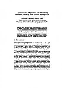
Let hP, Gi be a B1 -EPG representation of a graph G = (V, E). We say that paths Pv and Pu are adjacent paths if v and u are adjacent vertices in G, i.e., Pv and Pu share a common grid edge of G. We also say that G = EP G(hP, Gi). In B1 -EPG graphs, each vertex corresponds to a path of one of the following shapes: ⌞, ⌜, ⌟ or ⌝, allowing horizontal or vertical segments as well. We refer to a path of shape τ ∈ {⌞, ⌜, ⌝, ⌟, |, −} as an τ -path. We denote by P⌞ the collection of ⌞-paths in P, and similarly we use the notations P⌟ , P⌜ and P⌝ . For no-bend paths we complete the definition by referring them as ⌞-paths. Sometimes, it is of interest to consider even finer, more restrictive subclasses of B1 -EPG by limiting the type of bends that are allowed, namely, the subclasses formed by the subsets of the four single bend shapes (i.e., {⌞}, {⌟, ⌞}, {⌞, ⌝}, {⌞, ⌜, ⌝}, where all other subsets are isomorphic to these up to 90◦ rotation), allowing paths with no-bend as well. We denote these classes by ⌞-EPG, ⌟⌞-EPG, ⌞⌝-EPG and ⌞ ⌜ ⌝-EPG respectively. Let G be a ⌟⌞-EPG with grid representation hP, Gi. We define the lexicographic (LEX) order ≺ on the paths in P as follows; see Figure 1. For path Pv ∈ P we denote by ∂Pv the bottommostleftmost grid point that is contained in Pv , that is, ∂Pv = miny {minx {(x, y) ∈ Pv }}. We say that Pv ≺Pu if ∂Pv lies below ∂Pu or they both lie in the same row and ∂Pv is left of ∂Pu . We complete ≺ to a total order by arbitrarily breaking ties.

f

g c

h d

e a

b

Fig. 1. The LEX ordering of a ⌟⌞-EPG representation: a≺b≺c≺d≺e≺f ≺g≺h.

3 3.1

Coloring B1 -EPG Graphs Hardness result for coloring B1 -EPG graphs

In this section, we prove that coloring problem on B1 -EPG graphs is NP-complete by a reduction from the problem of coloring circle graphs which was shown to be NP-complete in [7]. We start by defining circle graphs. A circle graph is the intersection graph of a set of chords of a circle. That is, it is an undirected graph whose vertices can be associated with chords of a circle such that two vertices are adjacent if and only if the corresponding chords cross each other. We may assume without loss of generality that no two chords in the diagram of chords of the circle share a common endpoint. Coloring circle graphs remains NP-complete even if the graph is given by its chord model [7].

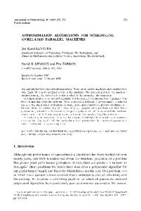
Theorem 1. Let G be a B1 -EPG graph. Coloring G with the exact number of colors χ(G) is NPcomplete. Proof. Let G be a circle graph. We construct a B1 -EPG representation for a graph G0 so that G is c-colorable if and only if G0 is. The construction is as follows; see Figures 2 and 3 for an illustration. We slide all the endpoints of the chords to the upper right quadrant of the circle, while preserving their order on the circle (thus, intersections are not changed under these transformations). Now, we replace each chord by an ⌞-shape bend path, where every vertex v in G corresponds to a path Pv with the same endpoints on the circle. Note that since we assumed that all endpoints are distinct, the horizontal segment of each path lies on a unique horizontal line, and the vertical segment lies on a unique vertical line. Moreover, the intersection points of pairs of paths are in one-to-one correspondence with the edges of the graph.

b b

a d

c

b

a d

d a b

c a d c

c (a)

(b)

Fig. 2. (a) A circle diagram. (b) Each chord is replaced by a single-bend path on the grid.

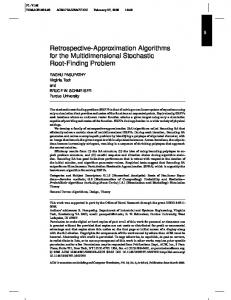
Consider an intersection point between two paths Pv and Pu in the representation, where the horizontal section of Pv intersects with the vertical segment of Pu . We split Pv at the intersection point into two disjoint parts; the left part is a ⌞-path, and the right one is a −-path. We complete the latter to a ⌞-path by joining it to a vertical segment that overlaps only Pu . We also add (c − 1) short −-paths overlapping only these two segments of the former path Pv . Perform this transformation for every intersection point, and let G0 be the B1 -EPG-graph of this transformed representation. This, of course, may have split Pv into several segments, Pv1 , Pv2 , . . . , Pvk , with consecutive segments Pvi and Pvi+1 being joined by such a set of (c − 1) short horizontal paths: a (c − 1)-clique in G0 overlapping only Pvi and Pvi+1 . See Figure 3 for an illustration. It is clear from the transformation that the obtained graph G0 is indeed a B1 -EPG graph. Moreover, the transformation can be performed in polynomial time and the size of G0 is polynomial in the size of G, since |V (G0 )| = n + ce ≤ n + n3 , where G has n vertices and e edges. We now claim that G is c-colorable if and only if G0 is c-colorable. Let ϕ : V 7→ {1, · · · , c} be a valid assignment of colors for G. Then to color G0 it suffices to (1) color each vertex from G0 that came from an original path Pv (including its vertical segment and all of its horizontal split segments Pv1 , . . . , Pvk ) with the color used in G, and (2) for each newly added (c − 1)-clique (the short segments overlapping only Pvi and Pvi+1 which have the same color in the construction), we can use the (c − 1) remaining colors. This clearly colors G0 in c colors.

Pv

Pu

Pu Pv i

Pvi+1 (c-1) clique

(a)

(b)

Fig. 3. (a) Intersecting paths. (b) The horizontal is “split” and “glued” using a (c − 1)-clique. We now show that if G0 is c-colorable then G is c-colorable. Assume we have a c-coloring of the graph G0 . Since the (c − 1)-clique connecting any Pvi and Pvi+1 requires (c − 1) colors, consequently, Pvi and Pvi+1 have the same remaining cth color. Moreover, let Pu be the path that intersects Pv in G and whose intersection point with Pv is the split point between Pvi and Pvi+1 , then Pu and Pvi+1 are adjacent in G0 , thus get distinct colors. Since the coloring of G0 is proper, it also gives a proper coloring of G: color the path representing v in G with the same (common) color of its split segments Pv1 , . . . , Pvk in G0 . This concludes the proof of the theorem. t u Observe that by our construction, the paths in G0 are either ⌞-paths or −-paths, we thus conclude: Corollary 2 Let G be a ⌞-EPG graph. Coloring G with the exact number of colors χ(G) is NPcomplete. 3.2

A 4-approximation algorithm for coloring B1 -EPG graphs

We start by presenting a “subroutine” in Algorithm 3.1 that computes an approximation solution for a ⌟⌞-EPG representation. We then apply it more generally to an arbitrary B1 -EPG representation. It is a greedy First-Fit algorithm using the LEX ordering ≺, defined in Section 2 so clearly, it produces a proper coloring. Lemma 1 will show that when used for a ⌟⌞-EPG graph, Algorithm 3.1 achieves a 2-approximation. We will use the notation c(v) for the color assigned to vertex v.

Algorithm 3.1 Greedy-⌟⌞-EPG-Coloring (Input: P = P⌟ ∪ P⌞ ) 1: for each Pv ∈ P (in increasing order ≺) do 2: c(v) ← least color not in use among v’s neighbors 3: return total number k of distinct colors used and the coloring

Applying Algorithm 3.1 to the representation in Figure 1 gives the coloring: c(a) = c(c) = c(f ) = 1; c(b) = c(e) = c(g) = 2; c(d) = c(h) = 3.

For every path Pv ∈ P we denote by Γe(Pv ) the collection of paths adjacent to Pv that have been colored by Algorithm 3.1 prior to Pv . When convenient, we refer to Γe(Pv ) as a set of vertices. The color assigned to Pv by Algorithm 3.1 is dependent only on the colors assigned to paths in Γe(Pv ), thus we have Observation 3. Observation 3 Let hP, Gi be a ⌟⌞-EPG representation of a graph G = (V, E), and let Pv and Pu be adjacent paths. If Pu ≺Pv , then Pv and Pu share at least one of two grid edges e1 and e2 as follows: – If Pv is a ⌞-path, then e1 and e2 are respectively the horizontal and vertical grid edges contained in Pv and attached to its bend point. – If Pv is a ⌟-path, then e1 is the left-most horizontal grid edge contained in Pv and e2 is the vertical grid edge attached to its bend point. – If Pv is a |-path, then e1 is the bottom-most vertical grid edge contained in Pv (e2 in this case is undefined). – If Pv is a −-path, then e1 is the left-most horizontal grid edge contained in Pv (e2 in this case is undefined). Lemma 1. Let G be a ⌟⌞-EPG graph, then Algorithm 3.1 uses at most 2χ(G) colors. Proof. Let k be the maximum color used by Algorithm 3.1, we show that k ≤ 2χ(G). Indeed, put G = (V, E) and let v ∈ V be a vertex for which c(v) = k. Notice that whenever Algorithm 3.1 colors a vertex, the assigned color is determined by its previous-colored neighbors Γe(Pv ). Notice that if Algorithm 3.1 colored v with color k, then k is the least color that not in use for any vertex u ∈ Γe(Pv ), thus k ≤ Γe(Pv ) + 1. Moreover, by Observation 3, we have that each path in Γe(Pv ) shares at least one of two specified grid edges contained in Pv (denoted e1 and e2 ). We conclude that at least half of the paths in Γe(Pv ) contain one of those edges and without loss of generality, we assume it is e1 . Now, observe that any collection of paths containing a common edge corresponds to a clique in G, in particular, those paths in Γe(Pv ) that contain e1 together with v itself, form a clique. We get 21 Γ˜ (v) + 1 ≤ ω(G) ≤ χ(G), thus k ≤ Γe(Pv ) + 1 < 2ω(G) ≤ 2χ(G), which completes the proof. t u Remark 1. Clearly, by rotating a representation by 180◦ , Algorithm 3.1 can be “turned” from Greedy-⌟⌞-EPG-Coloring into Greedy-⌝⌜-EPG-Coloring. We now use Algorithm 3.1 as a building block in Algorithm 3.2 in order to colors B1 -EPG graphs.

Algorithm 3.2 B1 -EPG Coloring 4-Approximation (Input: G = EP G(hP, Gi)) 1: Let P = P⌞ ∪ P⌟ ∪ P⌝ ∪ P⌜ 2: k1 ←Greedy-⌟⌞-EPG-Coloring(P⌞ ∪ P⌟ ) 3: k2 ←Greedy-⌝⌜-EPG-Coloring(P⌜ ∪ P⌝ ) // using different color names // 4: return total number of distinct colors used and the coloring

Algorithm 3.2 partitions the paths in P into two subsets P⌞ ∪P⌟ and P⌜ ∪P⌝ , each induces a subgraph of G, which is a ⌟⌞-EPG graph (denoted G1 and G2 respectively). Then, it colors each

of these two graphs G1 and G2 using Algorithm 3.1, with distinct “palettes” of colors. Clearly, the coloring produced by Algorithm 3.2 is proper. Notice that in order to color a graph G, one needs at least the maximum of χ(G1 ), χ(G2 ) colors. By Lemma 1, Algorithm 3.2 uses at most 2χ(G1 ) + 2χ(G2 ) ≤ 4χ(G) colors, we thus have Theorem 4 below. Theorem 4. Let G be a B1 -EPG graph, then Algorithm 3.2 uses at most 4χ(G) colors.

4 4.1

Maximum Independent Set on B1 -EPG Graphs Hardness result for finding maximum independent set on B1 -EPG Graphs

In this section, we show that the Maximum Independent Set on B1 -EPG graphs is NP-complete. We use a reduction from Maximum Independent Set on planar graphs with maximum degree four, which is known to be NP-complete [6]; our proof is inspired by [14]. Theorem 5. Maximum Independent Set on B1 -EPG graphs is NP-complete. Proof. Let G = (V, E) be a planar graph with maximum degree four; Maximum Independent Set on planar graph with maximum degree four is NP-complete [6]. We construct a B1 -EPG representation of a graph G0 = (V 0 , E 0 ) so that a maximum independent set in G0 corresponds to a maximum independent set in G and vice versa. Fix an embedding of G in a grid G such that edges of G are piecewise linear curves following the grid lines (such an embedding in a linear sized grid always exists and is constructible in polynomial time [16]). Each edge e ∈ E is thus corresponds to a path πe in the grid G, and denote by ke the number of segments (links) πe consists of. Note further, that these paths intersect only at their endpoints, namely, in the vertices of G since the embedding is planar.   Let G0 be a graph obtained from G by subdividing every edge e with 2 ke2+1 new vertices; we denote the set of new vertices corresponding to an edge e by Ue and by U the set of all such new vertices, we thus have V 0 = V ∪ U . Notice that since |Ue | is even for each edge e of G, a maximum independent set in G0 contains exactly half of the vertices in Ue , and at most one of the vertices corresponding to the “original” endpoints of e. We thus have X  ke + 1  α(G0 ) = α(G) + 2 e∈E

and thus to complete the proof it suffices to show that G0 is B1 -EPG graph. Having the grid embedding of G, we construct a B1 -EPG representation hP, Gi of G0 as follows; see Figure 4 for an illustration. We start by placing the vertices in U into G. Let e be an edge of G, by definition πe has ke − 1 bend points. At each such grid point we place one vertex from Ue , we also place one vertex from Ue in the interiors of the first and last links of πe . Finally, we place the remaining vertices of Ue arbitrarily along πe (the order in which the vertices are located along πe preserves adjacencies). When convenient we may refer to vertices of G0 as the grid points they are embedded to. We now associate each vertex v of G0 with a path Pv (which is either a single-bend path or a segment) so that Pv and Pu share an edge of G if and only if v and u are adjacent in G0 . For every v ∈ V , set Pv to be a short vertical segment around v. Let u ∈ U , then u has exactly two neighbors, and consider first the case where both are from U . We set Pu to be a path consisting of the two segments connecting u with each of its neighbors. If u is embedded to a bend point of

(a)

(b)

(a) A rectilinear grid embedding of some graph G0 ; vertices of V are grayed. (b) A B1 -EPG representation of G0 .

Fig. 4.

some πe , then Pu is a single-bend path, otherwise it is just a segment. Finally, let u ∈ U be a vertex with neighbors u0 ∈ U and v ∈ V (notice that by construction no vertex in G0 has more than one neighbor from V ) in this case, u, u0 , and v are embedded to the same grid row/column and we set Pu as follows, distinguishing between two subcases, according to whether all three vertices are embedded to the same column or row of G. (i) u, u0 , and v are on the same column: We set Pu to be a vertical segment that begins at u0 and almost reaches v (in such a way that it ends close enough to share a grid edge with Pv ). (ii) u, u0 , and v are on the same row: We set Pu to be a ⌟-path or a ⌜-path that starts at u0 and bends at v, sharing its vertical edge with Pv , avoiding other possible neighbors of v. It is easy to see that indeed for every u, v ∈ V 0 the paths Pu and Pv share a grid edge if and only if u and v are adjacent in G0 , thus the desired result follows. t u Remark 2. The proof of Theorem 5 can be modified so that it uses only two bend shapes; thus Maximum Independent Set is NP-complete already on ⌟⌞-EPG and on ⌞⌝-EPG graphs.

4.2

A 4-approximation algorithm for Maximum Independent Set on B1 -EPG Graphs

In this section we present a constant-factor approximation algorithm for Maximum Independent Set (Algorithm 4.2 below). In a similar way to Section 3.2, we start by presenting a “subroutine” that computes an approximated solution for a subgraph, and then use the subroutine in order to compute an approximated solution for the whole graph. This subroutine is described in Algorithm 4.1 below, which uses a standard greedy Independent Set algorithm (thus clearly, produces an Independent Set). Note that the order in which it examines the vertices is the reversed order of that used in Algorithm 3.1, namely, according to the decreasing order of ≺. Lemma 2 claims that when used for a ⌟⌞-EPG graph, Algorithm 4.1 computes a 2-approximation.

Algorithm 4.1 Greedy-⌟⌞-EPG-Independent-Set (Input: P = P⌟ ∪ P⌞ ) 1: S ← ∅ 2: for each Pu ∈ P (in decreasing order by ≺) do 3: add u to S and remove Pu from P 4: remove all paths corresponding to u’s neighbors from P 5: return S

Applying Algorithm 4.1 to the representation in Figure 1 gives the independent set: {h, g, d}. Lemma 2. Let G be a ⌟⌞-EPG graph, then Algorithm 4.1 finds a maximal independent set of size at least 12 α(G). Proof. Let hP, Gi be a ⌟⌞-EPG representation of a graph G = (V, E). Let OP T be a maximum independent set in G and let S be the maximal Independent Set returned by Algorithm 4.1. We claim that |OP T | ≤ 2|S|. Notice that for every v ∈ V the path Pv is removed from P at some point (in lines 3 or 4). Moreover, if a path Pv is removed from P in line 4, then its deletion must occur when the algorithm added to S some vertex u with v≺u. Equivalently, whenever the algorithm adds a vertex u to S, it removes from P paths Pv adjacent to Pu where v≺u (in this case, any other vertex v 0 adjacent to u with u≺v 0 has been already removed from S in an earlier stage, necessarily in line 4). By eliminating vertices in OP T ∩ S we may assume that OP T ∩ S = ∅. We therefore assume that the paths corresponding to vertices in OP T were all eliminated from P in line 4. We define a correspondence ϕ : OP T → S as follows: ϕ(v) = u where Pv was removed from P in line 4 as a consequence of adding u to S In particular, if ϕ(v) = u then u and v are adjacent and v≺u. We claim that for every u ∈ S there exist at most two distinct vertices v1 , v2 ∈ OP T with ϕ(v1 ) = ϕ(v2 ) = u and conclude that |OP T | ≤ 2|S|. Indeed, assume to the contrary that for some u ∈ S, there exist three vertices v1 , v2 , v3 ∈ OP T with ϕ(vi ) = u (i = 1, 2, 3). At least two of the three paths share with Pu a grid edge on the same direction; w.l.o.g., assume that Pv1 and Pv2 share a horizontal edge with Pu . We thus have that Pvi is adjacent to Pu and vi ≺u (i = 1, 2), and in particular Pu , Pv1 and Pv2 share a common edge (the leftmost-bottommost grid-edge contained in Pu ). However, as v1 and v2 are both in OP T , they are nonadjacent. – A contradiction. t u We now use Algorithm 4.1 as a building block in Algorithm 4.2 in order to find a maximal Independent Set in B1 -EPG graphs. Here too, as in Remark 1, by rotating a representation by 180◦ , Algorithm 4.1 can be “turned” from Greedy-⌟⌞-EPG-Independent-Set into Greedy-⌝⌜-EPGIndependent-Set. Theorem 6 claims that when used on a B1 -EPG graph, Algorithm 4.2 achieves a 4-approximation. Algorithm 4.2 B1 -EPG Independent Set 4-Approximation(G = hP, Gi) 1: let P = P⌞ ∪ P⌟ ∪ P⌝ ∪ P⌜ 2: S1 ←Greedy-⌟⌞-EPG-Independent-Set(P⌞ ∪ P⌟ ) 3: S2 ←Greedy-⌝⌜-EPG-Independent-Set(P⌜ ∪ P⌝ ) 4: return the largest amongst S1 , S2

Theorem 6. Let G be a B1 -EPG graph, then Algorithm 4.2 finds a maximal Independent Set of size at least 14 α(G). Proof. Let hP, Gi be a B1 -EPG representation of G. Put P = P⌞ ∪ P⌟ ∪ P⌝ ∪ P⌜ and let G1 and G2 be the ⌟⌞-EPG graphs with representations hP⌞ ∪ P⌟ , Gi and hP⌜ ∪ P⌝ , Gi, respectively. Clearly, α(G) ≤ α(G1 ) + α(G2 ). Let S1 and S2 be the sets computed in lines 2 and 3 of the algorithm. By Lemma 2, we get α(G) ≤ α(G1 ) + α(G2 ) ≤ 2|S1 | + 2|S2 | ≤ 4 max{|S1 |, |S2 |} which completes the proof.

5

t u

Concluding Remarks

We observe that Maximum Clique in B1 -EPG graphs can be optimally solved in polynomial time using a brute-force algorithm. In [9] the authors show that each clique in the graph has one of two forms in the B1 -EPG representation, referred to as “edge clique” and “claw clique”. An edge clique consists of all paths containing a given grid edge; a claw clique consists of all paths sharing two-out-of-three edges of a given claw centered at a given grid point (there are 4 different claws at each grid point.) Consequently, given a grid representation of a B1 -EPG graph G, one can simply examine each grid edge and count the number of paths containing that edge, and for each grid point and four corresponding claws, count the number of path containing two out of three edges of that claw. This can be done in time polynomial in the size of G, which may be assumed to be of size at most 2n × 2n for a B1 -EPG representation. This implies an O(n3 ) time algorithm for Maximum Clique given a B1 -EPG representation. A somewhat different approach can solve Maximum Clique for a B1 -EPG graph without being given representation based on the fact that the neighborhood of a vertex in B1 -EPG graph is weaklychordal [1]. It is well known that Maximum Clique in weakly-chordal graphs can be found in O(n4 ) time [15]. Since a maximum clique is contained in a closed neighborhood of each of its vertices, then this yields a O(n5 ) time algorithm for Maximum Clique given just the B1 -EPG graph and not the representation. In Algorithms 3.2 and 4.2 we used, respectively, Algorithms 3.1 and 4.1 with subgraphs induced by P⌞ ∪ P⌟ and P⌜ ∪ P⌝ . Taking into consideration also the two other options (i.e., P⌟ ∪ P⌝ and P⌜ ∪ P⌞ ) has no effect on the asymptotic quality of the solutions. However, as a heuristic, one might wish to apply the algorithm to both and take the better of the two. Algorithm 3.2 and Algorithm 4.2 are greedy. Both have ”bad” instances for which the factors mentioned here are tight. It is possible, of course, that a different approach may lead to better approximation factors. As open problems, we suggest that it would be interesting to find approximation algorithms to find a minimum dominating set or a maximum weighted independent set for B1 -EPG graphs.

References 1. A. Asinowski and B. Ries, Some properties of edge intersection graphs of single bend paths on a grid, Discrete Mathematics 312 (2012), 427–440. 2. A. Asinowski and A. Suk, Edge intersection graphs of systems of grid paths with bounded number of bends, Discrete Applied Mathematics 157 (2009), 3174–3180.

3. T. Biedl and M. Stern, On edge intersection graphs of k-bend paths in grids, Discrete Mathematics & Theoretical Computer Science (DMTCS) 12 (2010), 1–12 . 4. K. Cameron, S. Chaplick, and C. T. Hoang, Recognizing Edge Intersection Graphs of ⌞-Shaped Grid Paths, LAGOS 2013, to appear. 5. E. Cohen, M. C. Golumbic and B. Ries, Characterizations of cographs as intersection graphs of paths on a grid, submitted. 6. M. R. Garey and D. S. Johnson. Computers and Intractability: a Guide to the Theory of NPcompleteness. Freeman, San Francisco, 1979. 7. M. R. Garey, D. S. Johnson, G. L. Miller and C. Papadimitriou, The complexity of coloring circular arcs and chords, SIAM. J. on Algebraic and Discrete Methods 1 (1980), 216–227. 8. M. C. Golumbic, Algorithmic Graph Theory and Perfect Graphs, Academic Press, New York, 1980. Second edition: Annals of Discrete Mathematics 57, Elsevier, Amsterdam, 2004. 9. M. C. Golumbic, M. Lipshteyn, and M. Stern, Edge intersection graphs of single bend paths on a grid, Networks 54 (2009), 130–138. 10. M. M. Halld´ orsson, A still better performance guarantee for approximate graph coloring, Information Processing Letters 45 (1993), 19–23. 11. D. Heldt, K. Knauer and T. Ueckerdt, Edge-intersection graphs of grid paths: the bend-number, Arxiv preprint arXiv:1009.2861, arxiv.org, September 2010. 12. D. Heldt, K. Knauer and T. Ueckerdt, On the bend-number of planar and outerplaner graphs, Proceedings of 10th Latin American Symposium on Theoretical Informatics (LATIN 2012), 458–469. 13. A. Kako, T. Ono, T. Hirata and M. M. Halld´ orsson, Approximation algorithms for the weighted independent set problem in sparse graphs, Discrete Applied Mathematics 157 (2009), 617–626. 14. J. Kratochv´ıl and J. Neˇsetˇril, Independent set and clique problems in intersection-defined classes of graphs, Commentationes Mathematicae Universitatis Carolinae 31 (1990), 85–93. 15. J. P. Spinrad and R. Sritharan, Algorithms for weakly triangulated graphs, Discrete Appl. Math. 59 (1995) 181–191. 16. L. G. Valiant, Universality considerations in VLSI circuits, IEEE Trans. Comput. 30 (1981), 135–140.