Structural Rounding: Approximation Algorithms for Graphs Near an ...

Structural Rounding: Approximation Algorithms for Graphs Near an Algorithmically Tractable Class Erik D. Demaine1 , Timothy D. Goodrich2 , Kyle Kloster2 , Brian Lavallee2 , Quanquan C. Liu1 , Blair D. Sullivan2 , Ali Vakilian1 , and Andrew van der Poel2

arXiv:1806.02771v1 [cs.CC] 7 Jun 2018

1

MIT, Cambridge, MA, USA, {edemaine,quanquan,vakilian}@mit.edu 2 NC State University, Raleigh, NC, USA, {tdgoodri,kakloste,blavall,blair_sullivan,ajvande4}@ncsu.edu Abstract

We develop a new framework for generalizing approximation algorithms from the structural graph algorithm literature so that they apply to graphs somewhat close to that class (a scenario we expect is common when working with real-world networks) while still guaranteeing approximation ratios. The idea is to edit a given graph via vertex- or edge-deletions to put the graph into an algorithmically tractable class, apply known approximation algorithms for that class, and then lift the solution to apply to the original graph. We give a general characterization of when an optimization problem is amenable to this approach, and show that it includes many well-studied graph problems, such as Independent Set, Vertex Cover, Feedback Vertex Set, Minimum Maximal Matching, Chromatic Number, (`-)Dominating Set, and Edge (`-)Dominating Set. To enable this framework, we develop new editing algorithms that find the approximately fewest edits required to bring a given graph into one of several important graph classes (in some cases, also approximating the target parameter of the family). For bounded degeneracy, we obtain a bicriteria (4, 4)-approximation which also extends to a √ smoother log w))bicriteria trade-off. For bounded treewidth, we obtain a bicriteria (O(log1.5 n), O( √ approximation, and for bounded pathwidth, we obtain a bicriteria (O(log1.5 n), O( log w · log n))-approximation. For treedepth 2 (also related to bounded expansion), we obtain a 4approximation. We also prove complementary hardness-of-approximation results assuming P 6= NP: in particular, all of the problems just stated have a log-factor inapproximability, except the last which is not approximable below some constant factor (2 assuming UGC).

ACM Classifications: F.2.2 Nonnumerical Algorithms and Problems Keywords: structural rounding, graph editing, maximum subgraph problem, treewidth, degeneracy, APX-hardness, approximation algorithms

Contents 1 Introduction 1.1 Our Results: Structural Rounding . . . . . . . . . . . . . . . . . . . . . . . . . . 1.2 Our Results: Editing . . . . . . . . . . . . . . . . . . . . . . . . . . . . . . . . . . 1.3 Related Work . . . . . . . . . . . . . . . . . . . . . . . . . . . . . . . . . . . . . .

2 3 4 5

2 Techniques 2.1 Structural 2.2 Editing to 2.3 Editing to 2.4 Editing to 2.5 Editing to

6 6 7 7 7 8

Rounding Framework . . . . . . . Bounded Degeneracy and Degree . Bounded Weak c-Coloring Number Bounded Treewidth . . . . . . . . Treedepth 2 . . . . . . . . . . . . . 1

. . . . .

. . . . .

. . . . .

. . . . .

. . . . .

. . . . .

. . . . .

. . . . .

. . . . .

. . . . .

. . . . .

. . . . .

. . . . .

. . . . .

. . . . .

. . . . .

. . . . .

. . . . .

. . . . .

. . . . .

3 Preliminaries 3.1 Structural Graph Classes . . . . . . . . . . . 3.1.1 Degeneracy, cores, and shells . . . . 3.1.2 Weak coloring number . . . . . . . . 3.1.3 Treewidth, pathwidth, and treedepth 3.2 Editing Problems . . . . . . . . . . . . . . . 3.3 Hardness and Reductions . . . . . . . . . . 3.3.1 Approximation preserving reductions 3.3.2 Hard problems . . . . . . . . . . . . 3.4 Optimization Problems . . . . . . . . . . . .

. . . . . . . . .

. . . . . . . . .

. . . . . . . . .

. . . . . . . . .

. . . . . . . . .

. . . . . . . . .

. . . . . . . . .

. . . . . . . . .

. . . . . . . . .

. . . . . . . . .

. . . . . . . . .

. . . . . . . . .

. . . . . . . . .

. . . . . . . . .

. . . . . . . . .

. . . . . . . . .

. . . . . . . . .

. . . . . . . . .

. . . . . . . . .

. . . . . . . . .

. . . . . . . . .

8 8 8 9 9 10 11 11 12 13

4 Structural Rounding 4.1 General Framework 4.2 Vertex Deletions . 4.3 Edge Deletions . . 4.4 Edge Contractions

. . . .

. . . .

. . . .

. . . .

. . . .

. . . .

. . . .

. . . .

. . . .

. . . .

. . . .

. . . .

. . . .

. . . .

. . . .

. . . .

. . . .

. . . .

. . . .

. . . .

. . . .

14 14 15 18 19

. . . .

. . . .

. . . .

. . . .

. . . .

. . . .

. . . .

. . . .

. . . .

. . . .

. . . .

. . . .

. . . .

. . . .

5 Editing Algorithms 5.1 Degeneracy: Density-Based Bicriteria Approximation . . . . . . . . . . . . . . . . 5.1.1 Analysis overview and the local ratio theorem . . . . . . . . . . . . . . . . 4m−βrn 5.1.2 m−rn , β -approximation for vertex deletion . . . . . . . . . . . . . . . 5.2 Degeneracy: LP-based Bicriteria Approximation . . . . . . . . . . . . . . . . . . . 5.2.1 (3, 3)-approximation for edge deletion . . . . . . . . . . . . . . . . . . . . 5.2.2 (4, 4)-approximation for vertex deletion . . . . . . . . . . . . . . . . . . . 5.2.3 Integrality gap of DegenEdgeEdit-LP and DegenVertexEdit-LP . . 5.3 Treewidth/Pathwidth: Bicriteria Approximation for Vertex Editing . . . . . . . . √ 5.3.1 Treewidth: (O(log1.5 n), O( √log w))-approximation for vertex deletion . . 5.3.2 Pathwidth: (O(log1.5 n), O( log w·log n))-approximation for vertex deletion 5.4 Proof of Theorem 5.24 . . . . . . . . . . . . . . . . . . . . . . . . . . . . . . . . . 5.5 Bounded Degree: Polynomial Time Algorithm for Edge Editing . . . . . . . . . . 5.6 Treedepth 2: O(1)-approximation for Editing . . . . . . . . . . . . . . . . . . . .

19 19 20 21 23 23 25 26 27 28 30 30 31 32

6 Editing Hardness Results 6.1 Degeneracy: o(log n)-Inapproximability of Vertex Editing . . . . . . . . . . 6.2 Degeneracy: (ln r − C · ln ln r)-Inapproximability of Edge Editing . . . . . . 6.3 Weak Coloring Numbers: o(t)-Inapproximability of Editing . . . . . . . . . 6.4 Treewidth and Clique Number: o(log n)-Inapproximability of Vertex Editing 6.5 Bounded Degree: (ln d − C · ln ln d)-Inapproximability of Vertex Editing . . 6.6 Treedepth 2: (2 − ε)-Inapproximability of Vertex Editing . . . . . . . . . . 6.7 Treedepth 2: APX-hardness of Edge Editing . . . . . . . . . . . . . . . . . .

32 32 36 40 48 52 54 56

7 Open Problems

1

. . . . . . .

. . . . . . .

. . . . . . .

58

Introduction

Network science has empirically established that real-world networks (social, biological, computer, etc.) exhibit significant sparse structure. Theoretical computer science has shown that graphs with certain structural properties enable significantly better approximation algorithms for hard problems. Unfortunately, the experimentally observed structures and the theoretically required structures are generally not the same: mathematical graph classes are rigidly defined,

2

while real-world data is noisy and full of exceptions. This paper provides a framework for extending approximation guarantees from existing rigid classes to broader, more flexible graph families that are more likely to include real-world networks. Specifically, we hypothesize that most real-world networks are in fact small perturbations of graphs from a structural class. Intuitively, these perturbations may be exceptions caused by unusual/atypical behavior (e.g., weak links rarely expressing themselves), natural variation from an underlying model, or noise caused by measurement error or uncertainty. Formally, a graph is γ-close to a structural class C, where γ ∈ N, if some γ edits (e.g., vertex deletions, edge deletions, or edge contractions) bring the graph into class C. Our goal is to extend existing approximation algorithms for a structural class C to apply more broadly to graphs γ-close to C. To achieve this goal, we need two algorithmic ingredients: 1. Editing algorithms. Given a graph G that is γ-close to a structural class C, find a length f (γ) sequence of edits that edit G into C. When the structural class is parameterized (e.g., treewidth ≤ w), we may also approximate those parameters. 2. Structural rounding algorithms. Develop approximation algorithms for optimization problems on graphs γ-close to a structural class C by converting ρ-approximate solutions on an edited graph in class C into g(α, γ)-approximate solutions on the original graph.

1.1

Our Results: Structural Rounding

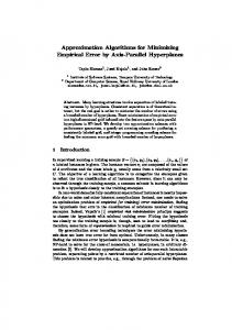
In Section 4, we give a general metatheorem giving sufficient conditions on an optimization problem to be amenable to the structural rounding framework. Specifically, if a problem Π has an approximation algorithm in structural class C, the problem and its solutions are “stable” under an edit operation, and there is an α-approximate algorithm for editing to C, then we get an approximation algorithm for solving Π on graphs γ-close to C. The new approximation algorithm incurs an additive error of O(γ), so we preserve PTAS-like (1 + ε) approximation factors provided γ ≤ δ OPTΠ for a suitable constant δ = δ(ε, α) > 0. For example, we obtain (1 + O(δ log1.5 n))-approximation algorithms for Vertex Cover, Feedback Vertex Set, Minimum Maximal Matching, and Chromatic Number on graphs (δ · OPTΠ (G))-close to having treewidth w via vertex deletions (generalizing exact algorithms for bounded treewidth graphs); and we obtain a (1−4δ)/(4r+1)-approximation algorithm Clique Number Degeneracy Weak 2-Coloring Number Weak c-Coloring Number Bounded Expansion

Bounded Degree

Treewidth Planar-Minor-Free Treedepth Star Forest

Figure 1: Illustration of hierarchy of structural graph classes used in this paper. 3

for Independent Set on graphs (δ · OPTΠ (G))-close to having degeneracy r (generalizing a 1/r-approximation for degeneracy-r graphs). These results use our new algorithms for editing to treewidth-w and degeneracy-r graph classes as summarized next.

1.2

Our Results: Editing

We develop editing approximation algorithms and/or hardness-of-approximation results for six well-studied graph classes: bounded clique number, bounded degeneracy, bounded treewidth/pathwidth, bounded treedepth, and bounded degree. Figure 1 summarizes the relationships among these classes, and Table 1 summarizes our results for each class. Graph Family Cλ Bounded Degree (d) Bounded Clique Number (b)

Bounded Degeneracy (r)

Bounded Weak c-Coloring Number (t) Bounded Treewidth (w)

Bounded Pathwidth (w)

Star Forest

Edit Operation ψ Edge Deletion

Vertex Deletion d-BDD-V O(log d)-approx. [25] (ln d − C · ln ln d)-inapprox. b-CN-V – o(log n)-inapprox. for b ∈ Ω(n1/2 ) r-DE-V

d-BDD-E Polynomial time [39]

–

–

–

r-DE-E

4m−βrn , β -approx. m−rn 1 2 ε , 1−ε -approx. (ε < 1)

o(log n)-inapprox. t-BWE-V-c – o(t)-inapprox. for t ∈ o(log n) w-TW-V √ (O(log1.5 n), O( log w))approx. o(log n)-inapprox. for w ∈ Ω(n1/2 ) w-PW-V √ (O(log1.5 n), O( log w · log n))approx. – SF-V 4-approx. (2 − ε)-inapprox. (UGC)

Edge Contraction

1 2 ε , 1−2ε

-approx. (ε < 1/2)

(ln r − C · ln ln r)-inapprox.

t-BWE-E-c – o(t)-inapprox. for t ∈ o(log n) w-TW-E (O(log n log log n), O(log w))approx. [3] – w-PW-E (O(log n log log n), O(log w · log n))approx. [3] – SF-E 3-approx. APX-complete

–

t-BWE-C-c – o(t)-inapprox. for t ∈ o(log n) –

–

–

Table 1: Summary of results for (C, ψ)-Edit problems (and their abbreviations). “Approx.” denotes a polynomial-time approximation or bicriteria approximation algorithm; “inapprox.” denotes inapproximability assuming P 6= NP unless otherwise specified. Hardness results. We begin by showing that vertex- and edge-deletion to degeneracy r (rDE) are o(log n)- and (ln r − C · ln ln r)-inapproximable, respectively, where C > 0 is a constant. These results are shown with a strict reduction from Set Cover. A similar reduction proves that d-Bounded-Degree Deletion is (ln d − C · ln ln d)-inapproximable for target maximum degree d, for a constant C > 0; coupled with [25], this establishes that (log d) is nearly tight. Additionally, we show that editing a graph to have a specified weak c-coloring number, a generalization of degeneracy, is o(t)-inapproximable, again using a similar strict reduction from Set Cover. The problems of vertex editing to treewidth w and clique number b are each shown to be o(log n)-inapproximable when the target parameter is Ω(nδ ) for a constant δ ≥ 1/2; these results also follow a strict reduction from Set Cover. Note that since computing treewidth (similarly, clique number and weak c-coloring number) is NP-hard, trivially it is not possible to find any polynomial time algorithm for the problem of editing to treewidth w with finite approximation guarantee. In particular, this implies that we cannot hope for anything better than bicriteria approximation algorithms in these problems. Moreover, our hardness results for these problems show that even if the optimal edit set is guaranteed to be large, i.e., polynomial in the size of input graph, n, we cannot achieve approximation factor better than Ω(log n). 4

Finally, star forest (treedepth 2) is shown to be (2 − ε)-inapproximable for vertex editing, via an L-reduction from vertex cover assuming the Unique Games Conjecture, and APX-complete for edge editing, via an L-reduction from bounded-degree minimum dominating set. Positive results. Complementing our hardness result for r-DE, we present two bicriteria approximation algorithms for r-DE-V, one using the local ratio theorem and another LP-rounding. While all three approximations can be tuned with error values, they yield constant (4, 4)- and (3, 3)-approximations for vertex and edge editing, respectively. Using vertex separators, we show a bicriteria approximation for vertex editing to bounded treewidth and pathwidth. Finally, using a hitting-set approach to delete forbidden subgraphs, we show 4- and 3-approximations for the vertex and edge deletion variants of editing to star forests.

1.3

Related Work

Editing graphs into a desired graph class is an active field of research and has various applications outside of graph theory, including computer vision and pattern matching [33]. We study the problem of deleting a minimum set X of vertices (edges) in an input graph G such that the result G[V \ X] has a specific property. Previous work studied this problem from the perspective of identifying the maximum induced subgraph of G that satisfies a desired “non-trivial, hereditary” property, π [51, 54, 55, 77]. A graph property π is non-trivial if and only if infinitely many graphs satisfy π and infinitely many do not, and π is hereditary if G satisfying π implies that every induced subgraph of G satisfies π. The vertex-deletion problem for any non-trivial, hereditary property has been shown to be NP-complete [55] and even requires exponential time to solve, assuming the ETH [49]. Approximation algorithms for such problems have also been studied somewhat [31, 57, 68] in this domain, but in general this problem requires additional restrictions on the input graph and/or output graph properties in order to develop fast algorithms [16, 22, 23, 40, 50, 61, 62, 76]. For example, Dabrowski et al. [16] found that editing a graph to have a given degree sequence is W[1]-complete, but if one additionally requires that the final graph be planar, the problem becomes FPT. Mathieson [61] showed that editing to degeneracy d is W[P]-hard (even if the original graph has degeneracy d + 1 or maximum degree 2d + 1), but suggests that classes which offer a balance between the overly rigid restrictions of bounded degree and the overly global condition of bounded degeneracy (e.g., structurally sparse classes such as H-minor-free and bounded expansion [67]) may still be FPT. Some positive results on the parameterized complexity of editing to classes can be found in Drange’s 2015 PhD thesis [22]; in particular, the results mentioned include parameterized algorithms for a variety of NP-complete editing problems such as editing to threshold and chain graphs [23], star forests [23], multipartite cluster graphs [29], and H-free graphs given finite H and bounded indegree [24]. For a more comprehensive overview of the literature in this area, refer to Drange’s thesis [22]. Our approach differs from this prior work in that we focus on approximations of edit distance where the running time is not parameterized by any of the parameters in our edit problems, but rather fully polynomial-time approximation algorithms. The only previous results about approximate edit distance are by Fomin et al. [30] and a very recent result regarding approximate edit distance to bounded treewidth graphs [35]. Fomin et al. [30] provided two types of algorithms for vertex editing to planar F-minor-free graphs: a randomized algorithm that runs in O(f (F) · mn) time with an approximation constant cF that depends on F, as well as a fixed-parameter algorithm parameterized by the size of the edit set whose running time thus has an exponential dependence on the size of this edit set. Gupta et al. [35] strengthen the results in [30] but only in the context of parameterized approximation algorithms. Namely, they provide the following improvements on the results given in [30] as well as the following main results. They give a deterministic fixed-parameter

5

algorithm for Planar F-Deletion that runs in f (F) · n log n + nO(1) time and an O(log k)approximation where k is the maximum number of vertices in any planar graph in F; this implies 2 a fixed-parameter O(log w)-approximation algorithm with running time 2O(w log w) · n log n + nO(1) for w-Treewidth Vertex Deletion and w-Pathwidth Vertex Deletion. They also show that w-Treewidth Edge Deletion and w-Pathwidth Edge Deletion have parameterized algorithms that give an absolute constant factor approximation but with running times parameterized on w and the degree of the graph deg(G) [35]. Finally, they show that when F is the set of all connected graphs with three vertices, deleting the minimum number of edges to exclude F as a subgraph, minor, or immersion is APX-hard for bounded degree graphs [35]. Again, these running times are weaker than our results, which give bicriteria approximation algorithms that are polynomial without any parameterization on the treewidth or pathwidth of the target graphs. In a similar regime, Bansel et al. [3] studied w-Treewidth Edge Deletion (which implies an algorithm for w-Pathwidth Edge Deletion) and designed an LP-based bicriteria approximation for this problem. For a slightly different set of problems in which the goal is to exclude a single graph H as a subgraph (H-Vertex-Deletion), there exists a simple kapproximation algorithm. On the hardness side, Guruswami and Lee [36] proved that whenever H is 2-vertex-connected, it is NP-hard to approximate H-Vertex-Deletion within a factor of (|V (H)| − 1 − ε) for any ε > 0 (|V (H)| − ε assuming UGC). Moreover, when H is a star or simple 3 path with k vertices, O(log k)-approximation algorithms with running time 2O(k log k) · nO(1) are known [36, 52]. Other related work. An important special case of the problem of editing graphs into a desired class is the minimum planarization problem, in which the target class is planar graphs. One application of minimum planarization is approximating the well-known crossing number problem [15]. Refer to [5, 11, 14, 41, 45, 44, 60, 74] for the recent developments on minimum planarization and crossing number. Prior to our work, the idea of designing efficient algorithms for optimization problems on graphs near a structural class was considered for only a limited class of problems and family of graphs. For instance, Magen and Moharrami [59] developed a PTAS algorithm for estimating the size of Independent Set (IS) in a “noisy setting” which they defined as a class of graphs constructed by adding δn edges to minor closed families of graphs (for sufficiently small values of δ). Later, Chan and Har-Peled [9] developed a PTAS algorithm that returns a (1 + ε)approximation to IS in noisy planar graphs. Very recently, Bansel et al. [3] developed an LP-based approach for noisy minor-closed IS whose runtime and approximation factor achieve better dependence on δ. Moreover, they provide a similar guarantee for noisy Max k-CSPs (graphs near minor-closed families).

2

Techniques

This section summarizes the main techniques, ideas, and contributions in the rest of the paper.

2.1

Structural Rounding Framework

The main contribution of our structural rounding framework (Section 4) is to get the right definitions that make for a broadly applicable framework with precise approximation guarantees. Our framework supports arbitrary graph edit operations and both minimization and maximization problems, provided they jointly satisfy two properties: a combinatorial property called “stability” and an algorithmic property called “structural lifting”. Roughly, these properties bound the amount of change that OPT can undergo from each edit operation, but they are also parameterized to enable us to derive tighter bounds when the problem has additional structure. With

6

the right definitions in place, the framework is simple: edit to the target class, apply existing approximation algorithm, and lift. The rest of the section shows that this framework applies to many different graph optimization problems. In particular, we verify the stability and structural lifting properties, and combine all the necessary pieces, including our editing algorithms from Section 5 and existing approximation algorithms for structural graph classes. Table 2 on page 16 summarizes all of these results.

2.2

Editing to Bounded Degeneracy and Degree

We present two constant-factor bicriteria approximation algorithms for finding the fewest vertex or edge deletions to reduce the degeneracy to a target threshold r. The first approach (Section 5.1) uses the local ratio technique by Bar-Yehuda et al. [4] to establish that good-enough local choices result in a guaranteed approximation. The second approach (Section 5.2) is based on rounding a linear-programming relaxation of an integer linear program. The integrality gap of this LP is Ω(n), which explains why we can hope only for bicriteria approximations via this approach. On the lower bound side, we show o(log n)-approximation is impossible for vertex edits (Section 6.1) and o(log r)-approximation is impossible for edge edits (Section 6.2) when we forbid bicriteria approximation, i.e., when we must match the target degeneracy r exactly. This result is based on a reduction from Set Cover. A similar reduction proves o(log d)-inapproximability of editing to maximum degree d, which proves tightness (up to constant factors) of a known O(log d)-approximation algorithm [25]. This algorithm is also LP-based, employing LLL-based analysis to show that the standard randomized rounding approach works. Unfortunately, because the integrality gap of our degeneracy LP is Ω(n), we cannot hope for such a result for editing to bounded degeneracy.

2.3

Editing to Bounded Weak c-Coloring Number

Weak c-coloring number is the key structure used to define bounded expansion, and nicely generalizes the notion of bounded degeneracy, which corresponds to c = 1. (Note, however, that larger c values make for smaller graph classes; see Section 3.1.2 for details.) In Section 6.3, we show that (non-bicriteria) o(log n)-approximation is NP-hard for any c ≥ 2, by adapting our proof of lower bound for bounded degeneracy. This hardness result applies to vertex and edge deletions, as well as edge contractions.

2.4

Editing to Bounded Treewidth

In Section 5.3, we present a bicriteria approximation algorithms for finding the fewest vertex to reduce the treewidth to a target threshold w. Our approach builds on the deep separator structure inherent in treewidth. We combine ideas from Bodleaender’s O(log n)-approximation algo√ rithm for treewidth with Feige et al.’s O( log w)-approximation algorithm for vertex separators √ [27] (where w is the target treewidth). In the end, we obtain a bicriteria (O(log1.5 n), O( log w))approximation that runs in polynomial time on all graphs (in contrast to many previous treewidth algorithms). The tree decompositions that we generate√are guaranteed to have O(log n) height. As a result, we also show a bicriteria (O(log1.5 n), O( log w · log n))-approximation result for pathwidth, based on the fact that the pathwidth is at most the width times the height of a tree decomposition. On the lower bound side (Section 6.4), we prove a o(log w)-inapproximability result by a different reduction from Set Cover. By a small modification, this lower bound also applies to editing to bounded clique number.

7

Editing to Treedepth 2

2.5

As a warmup to general treedepth results, we study the simple case of editing to graphs of treedepth 2, which are star forests. Here we do not need bicriteria approximation, though the problem remains hard, even to approximate within a constant factor. Assuming the Unique Games Conjecture, we show in Section 6.6 that Vertex Cover reduces to this editing problem without loss in OPT, implying a factor-2 lower bound for vertex edits. We also show APXhardness for edge edits (Section 6.7). Our constant-factor approximation (Section 5.6) is based on a reduction to Hitting Set.

3

Preliminaries

This section defines several standard notions and graph classes, and is probably best used as a reference. The one exception is Section 3.2, which formally defines the graph-class editing problem (Cλ , ψ)-Edit introduced in this paper. Graph notation. We consider finite, loopless, simple graphs. Unless otherwise specified, we assume that graphs are undirected and unweighted. We denote a graph by G = (V, E), and set n = |V |, m = |E|. Given G = (V, E) and two vertices u, v ∈ V we denote edges by e(u, v) or (u, v). We write N (v) = {u | (u, v) ∈ E} for the set of neighbors of a vertex v; the degree of v is deg(v) = |N (v)|. In digraphs, in-neighbors and out-neighbors of a vertex v are defined using edges of the form (u, v) and (v, u), respectively, and we denote in- and out-degree by deg- (v), deg+ (v), respectively. For the maximum degree of G we use ∆(G), or just ∆ if context is clear. The clique number of G, denoted ω(G), is the size of the largest clique in G.

3.1

Structural Graph Classes

In this section, we provide the necessary definitions for several structural graph classes (illustrated in Figure 1). 3.1.1

Degeneracy, cores, and shells

Definition 3.1. A graph G is r-degenerate if every subgraph of G contains a vertex of degree at most r; the degeneracy is the smallest r ∈ N+ so that G is r-degenerate, and we write degen(G) = r. Much of the literature on degeneracy is in the context of the more general notion of k-cores. Definition 3.2. For a graph G and positive integer r, the r-core of G is the maximal subgraph of G with minimum degree r. The r-shell of G is the set of vertices that are in the r-core of G but not in the (r + 1)-core of G. Lemma 3.1 ([13, 56, 63]). Given a graph G = (V, E), the following are equivalent: 1. The degeneracy of G is at most r. 2. The (r + 1)-core of G is empty. 3. There exists an orientation of the edges in E so that deg+ (v) ≤ r for all v ∈ V .

4. There exists an ordering {v1 , · · · , vn } of V so the degree of vj in G[{vj , · · · , vn }] is at most r.

It immediately follows that a graph G has degeneracy r if and only if r is the largest number such that the r-core of G is non-empty. We note that having bounded degeneracy immediately implies bounded clique and chromatic numbers ω(G), χ(G) ≤ degen(G) + 1 (the latter follows from a greedy coloring using the ordering from Lemma 3.1). 8

3.1.2

Weak coloring number

The weak c-coloring number was introduced along with the c-coloring number by Kierstead and Yang in [47], and it generalizes the notion of degeneracy in the following sense. As described in Lemma 3.1, the degeneracy of a graph can be understood as a worst-case bound, given any ordering of vertices, on the number of vertices that any given vertex v can “reach” via a path of length 1 in a DAG defined by an ordering of vertices (where edges are directed from vertices that occur earlier in the ordering to vertices that occur later). The weak c-coloring number instead bounds the number of vertices v reachable from u via a path of length at most c consisting of vertices that occur earlier than v in an ordering of the vertices. In fact, the weak 1-coloring number and degeneracy are equivalent notions. Definition 3.3. (Section 2 [47]) Let G be a finite, simple graph, let L : V (G) → N be an injective function defining an ordering on the vertices of G, and let Π(G) be the set of all possible such orderings. A vertex v is weakly c-reachable from u if there exists a uv-path P such that |P | ≤ c and for all w ∈ P , L(w) ≤ L(v), and we use wreachc (G, L, u) to denote the set of all such vertices. Let wscorec (G, L) be the maxu∈V (G) | wreachc (G, L, u)|. The weak c-coloring number of G is defined as wcolc (G) = minL∈Π(G) wscorec (G, L). The weak coloring number also provide useful characterizations for other graph classes as summarized in the following Lemma 3.2. Lemma 3.2 ([34, 67, 42, 78]). The generalized coloring numbers characterizes the graph class C for each of the following: c (G)) 1. C is nowhere dense ⇐⇒ lim lim sup log(wcol = 0. log |G|

c→∞

G∈C

2. C has bounded expansion ⇐⇒ ∃ a function f, ∀G ∈ C, ∀c ∈ N : wcolc (G) ≤ f (c). 3. C has treedepth bounded by k ⇐⇒ ∀G ∈ C, ∀c ∈ N : wcolc (G) ≤ k.

Additionally, the treewidth of a graph provides anupper bound on its weak coloring numbers. If a graph G has treewidth k, then wcolc (G) ≤ k+c k , and there is an infinite family of graphs such that this bound is tight [34]. 3.1.3

Treewidth, pathwidth, and treedepth

Perhaps the most heavily studied structural graph class is that of bounded treewidth; in this subsection we provide the necessary definitions for treewidth, pathwidth (when the idealized structure is restricted to being a path), and treedepth. Bounded treedepth is a stronger structural property than bounded pathwidth, and intuitively measures how “shallow” a tree the graph can be embedded in when edges can only occur between ancestor-descendent pairs. Definition 3.4 ([72]). Given a graph G, a tree decomposition of G consists of a collection Y of subsets (called bags) of vertices in V (G) together with a tree T = (Y, E) whose nodes Y correspond to bags which satisfy the following properties: S 1. Every v ∈ V (G) is contained in a bag B ∈ Y (i.e. B∈Y B = V ). 2. For all edges (u, v) ∈ E(G) there is a bag B ∈ Y that contains both endpoints u, v.

3. For each v ∈ V (G), the set of bags B ∈ Y containing v form a connected subtree of T (i.e. {B|v ∈ B, B ∈ Y} forms a subtree of T ). The width of a tree decomposition is maxB∈Y |B| − 1, and the treewidth of a graph G, denoted tw(G), is the minimum width of any tree decomposition of G.

9

Definition 3.5 ([72]). A path decomposition is a tree decomposition in which the tree T is a path. The pathwidth of G, denoted pw(G), is the minimum width of any path decomposition of G. Definition 3.6 ([66]). A treedepth decomposition of a graph G is an injective mapping ψ : V (G) → V (F ) of the vertices of G to the vertices of a rooted forest F such that for each edge (u, v) ∈ E(G), ψ(u) is either an ancestor or a descendant of ψ(v). The depth of a treedepth decomposition is the height of the forest F . The treedepth of G is the minimum depth of any treedepth decomposition of G. All graphs that exclude a simple fixed planar minor H have bounded treewidth, indeed, treewidth |V (H)|O(1) [10]. Thus, every planar-H-minor-free graph class is a subclass of some bounded treewidth graph class.

3.2

Editing Problems

This paper is concerned with algorithms that edit graphs into a desired structural class, while guaranteeing an approximation ratio on the size of the edit set. Besides its own importance, editing graphs into structural classes plays a key role in our structural rounding framework for approximating optimization problems on graphs that are “close” to structural graph classes (see Section 4). The basic editing problem is defined as follows relative to an edit operation ψ such as vertex deletion, edge deletion, or edge contraction: (C, ψ)-Edit Input: An input graph G = (V, E), family C of graphs, edit operation ψ Problem: Find k edits ψ1 , ψ2 , . . . , ψk such that ψk (ψk−1 (· · · ψ2 (ψ1 (G)) · · · )) ∈ C. Objective: Minimize k The literature has limited examples of approximation algorithms for specific edit operations and graph classes. Most notably, Fomin et al. [30] studies (C, ψ)-Edit for vertex deletions into the class of planar-H-minor-free graphs (graphs excluding a fixed planar graph H).1 In addition to fixed-parameter algorithms (for whenk is small), they give a cH -approximation |V (H)|3

algorithm for (C, ψ)-Edit where the constant cH = Ω 22 is rather large. Most of the graph classes we consider consist of graphs where some parameter λ (clique number, maximum degree, degeneracy, weak c-coloring number, or treewidth) is bounded. Thus we can think of the graph class C as in fact being a parameterized family Cλ . (For planar-Hminor-free, λ could be |V (H)|.) In addition to approximating just the number of edits, we can also loosen the graph class we are aiming for, and approximate the parameter value λ for the family Cλ . Thus we obtain a bicriteria problem which can be formalized as follows: (Cλ , ψ)-Edit Input: An input graph G = (V, E), parameterized family Cλ of graphs, a target parameter value λ∗ , edit operation ψ Problem: Find k edits ψ1 , ψ2 , . . . , ψk such that ψk (ψk−1 (· · · ψ2 (ψ1 (G)) · · · )) ∈ Cλ . Objective: Minimize k and λ ≥ λ∗ Definition 3.7. An algorithm for (Cλ , ψ)-Edit is a (bicriteria) (α, β)-approximation if it guarantees that the number of edits is at most α times the optimal number of edits into Cλ , and that λ ≤ β · λ∗ . 1 More generally, Fomin et al. [30] consider editing to the class of graphs excluding a finite family F of graphs at least one of which is planar, but as we just want the fewest edits to put the graph in some structural class, we focus on the case |F| = 1.

10

See Table 1 for a complete list of the problems considered, along with their abbreviations.

3.3

Hardness and Reductions

One of our contributions in this paper is providing hardness of approximation for several important instances of (C, ψ)-Edit defined in Section 3.2. Here, we describe the necessary definitions for approximation-preserving reductions as well as known approximability hardness results for several key problems. 3.3.1

Approximation preserving reductions

A classic tool in proving approximation hardness is the L-reduction, which linearly preserve approximability features [70], and imply PTAS reductions. Definition 3.8. Let A and B be minimization problems with cost functions CostA and CostB , respectively. An L-reduction is a pair of functions f and g such that: 1. f and g are polynomial time computable, 2. for an instance x of A, f (x) is an instance of B, 3. for a feasible solution y 0 of B, g(y 0 ) is a feasible solution of A, 4. there exists a constant c1 such that OPT(f (x)) ≤ c1 OPT(x), B

(1)

A

5. and there exists a constant c2 such that 0 CostA (g(y )) − OPT(x) ≤ c2 CostB (y ) − OPT(f (x)) . 0

A

B

(2)

In many cases, we will establish a stronger form of reduction known as a strict reduction, which implies an L-reduction [48, 69]. Definition 3.9. Let A and B be minimization problems with cost functions CostA and CostB , respectively. A strict reduction is a pair of functions f and g such that: 1. f and g are polynomial time computable, 2. for an instance x of A, f (x) is an instance of B, 3. for a feasible solution y 0 of B, g(y 0 ) is a feasible solution of A, 4. and it holds that CostA (g(y 0 )) CostB (y 0 ) ≤ . OPTA (x) OPTB (f (x))

(3)

We note that to prove a strict reduction, it suffices to demonstrate that OPTA (x) = OPTB (f (x)) and CostA (g(y 0 )) ≤ CostB (y 0 ).

11

3.3.2

Hard problems

As mentioned earlier, our approximation hardness results for the instances of (C, ψ)-Edit studied in this paper are via reductions from Set Cover, Vertex Cover and Minimum Dominating Set-B (Minimum Dominating Set in graphs of maximum degree B). We now formally define each of these, and state the associated hardness of approximation results used. Set Cover (SC) Input: A universe U of elements and a collection F of subsets S of the universe. Problem: Find a minimum size subset X ⊆ F that covers U; S∈X S = U. Theorem 3.3 ([21, 26, 58, 64, 65]). It is NP-hard to approximate Set Cover(U, F) within a factor of (1 − ε) ln(|U|) for any ε > 0. Moreover, this holds for instances where |F| ≤ poly(|U|). We remark that this result is tight, because there exists an (ln |U|)-approximation algorithm for SC [43]. Theorem 3.4 ([75]). There exists a constant C > 0 where it is NP-hard to approximate Set Cover(U, F) within a factor of (ln ∆ − C ln ln ∆), where ∆ = maxS∈F |S|. Moreover, in the hardness instances, ∆ ≥ fmax where fmax is the maximum frequency of an element of U in F. k-uniform Set Cover (k-uSC) Input: A universe U of elements and a collection F of subsets of the universe such that every element of U is contained in exactly k sets S in F. Problem: Find a minimum size subset X ⊆ F that covers U; S∈X S = U. Theorem 3.5 (Theorem 1.1 [19]). For any fixed k ≥ 3, it is NP-hard to approximate k-uSC to within a factor of (k − 1 − ε) for any ε > 0. Note that k is assumed to be constant with respect to |U| in this result. However, the same paper provides a slightly weaker hardness result when k is super-constant with respect to |U|. Theorem 3.6 (Theorem 6.2 [19]). There exists a constant b > 0 such that there is no polynomial time algorithm for approximating k-uniform Set Cover to within a factor of (bk/2c − 0.01) when 4 ≤ k ≤ (log |U|)1/b , unless NP ⊆ DTIME(nO(log log n) ). In particular, this holds for instances where |F| ≤ |U|. Vertex Cover (VC) Input: A graph G = (V, E). Problem: Find a minimum size set of vertices X ⊆ V s.t. G[V \ X] has no edge. Theorem 3.7 ([20, 46]). It is NP-hard to approximate Vertex Cover within a factor of 1.3606. Moreover, assuming the Unique Games Conjecture (UGC), VC cannot be approximated within any constant factor better than 2. Minimum Dominating Set-B (DSB) Input: An undirected graph G = (V, E) with degree bounded by B. Problem: Find a minimum size set of vertices C ⊆ V such that every vertex in V is either in C or is adjacent to a vertex in C.

12

Theorem 3.8 ([75]). There are constants C > 0 and B0 ≥ 3 such that for every B ≥ B0 it is NP-hard to approximate the Minimum Dominating Set-B problem within a factor of ln B − C ln ln B. The best known constants for small B in Theorem 3.8 are given in [12].

3.4

Optimization Problems

We conclude our preliminaries with formal definitions of several additional optimization problems for which we give new approximation algorithms via structural rounding in Section 4. `-Dominating Set (`-DS) Input: An undirected graph G = (V, E) and a positive integer `. Problem: Find a minimum size set of vertices C ⊆ V s.t. every vertex in V is either in C or is connected by a path of length at most ` to a vertex in C. Note when ` = 1 we call this Dominating Set. Edge `-Dominating Set (`-EDS) Input: An undirected graph G = (V, E) and a positive integer `. Problem: Find a minimum size set of edges C ⊆ V s.t. every edge in E is either in C or is connected by a path of length at most ` to an edge in C. Note when ` = 1 we call this Edge Dominating Set. `-Independent Set (`-IS) Input: A graph G = (V, E). Problem: Find a maximum size set of vertices X ⊆ V s.t. no two vertices in X are connected by a path of length ≤ `. Note when ` = 1 we call this Independent Set. Feedback Vertex Set (FVS) Input: A graph G = (V, E). Problem: Find a minimum size set of vertices X ⊆ V s.t. G \ X has no cycles. Minimum Maximal Matching (MMM) Input: A graph G = (V, E). Problem: Find a minimum size set of edges X ⊆ E s.t. X is a maximal matching. Chromatic Number (CRN) Input: A graph G = (V, E). Problem: Find a minimum size coloring of G s.t. adjacent vertices are different colors.

13

4

Structural Rounding

In this section, we show how approximation algorithms for a structural graph class can be extended to graphs that are near that class, provided we can find a certificate of being near the class. These results thus motivate our results in later sections about editing to structural graph classes. Our general approach, which we call structural rounding , is to apply existing approximation algorithms on the edited (“rounded”) graph in the class, then “lift” that solution to solve the original graph, while bounding the loss in solution quality throughout.

4.1

General Framework

First we define our notion of “closeness” in terms of a general family ψ of allowable graph edit operations (e.g., vertex deletion, edge deletion, edge contraction): Definition 4.1. A graph G0 is γ-editable from a graph G under edit operation ψ if there is a sequence of k ≤ γ edits ψ1 , ψ2 , . . . , ψk of type ψ such that G0 = ψk (ψk−1 (· · · ψ2 (ψ1 (G)) · · · )). A graph G is γ-close to a graph class C under edit operation ψ if some G0 ∈ C is γ-editable from G under ψ. To transform an approximation algorithm for a graph class C into an approximation algorithm for graphs γ-close to C, we will need two properties relating the optimization problem and the type of edits:2 Definition 4.2. A graph minimization (resp. maximization) problem Π is stable under an edit operation ψ with constant c0 if OPTΠ (G0 ) ≤ OPTΠ (G)+c0 γ (resp. OPTΠ (G0 ) ≥ OPTΠ (G)−c0 γ) for any graph G0 that is γ-editable from G under ψ. In the special case where c0 = 0, we call Π closed under ψ. When ψ is vertex deletion, closure is equivalent to the graph class defined by OPTΠ (G) ≤ λ (resp. OPTΠ (G) ≥ λ) being hereditary; we also call Π hereditary. Definition 4.3. A minimization (resp. maximization) problem Π can be structurally lifted with respect to an edit operation ψ with constant c if, given any graph G0 that is γ-editable from G under ψ, and given the corresponding edit sequence ψ1 , ψ2 , . . . , ψk with k ≤ γ, a solution S 0 for G0 can be converted in polynomial time to a solution S for G such that CostΠ (S) ≤ CostΠ (S 0 ) + c · k (resp. CostΠ (S) ≥ CostΠ (S 0 ) − c · k). Now we can state the main result of structural rounding: Theorem 4.1 (Structural Rounding Approximation). Let Π be a minimization (resp. maximization) problem that is stable under the edit operation ψ with constant c0 and that can be structurally lifted with respect to ψ with constant c. If Π has a ρ(λ)-approximation algorithm in the graph class Cλ , and (Cλ , ψ)-Edit has a polynomial-time (α, β)-approximation algorithm, then there is a polynomial-time ((1 + c0 αδ) · ρ(βλ) + cαδ)-approximation (resp. ((1 − c0 αδ) · ρ(βλ) − cαδ)approximation) for Π on any graph that is (δ · OPTΠ (G))-close to the class Cλ . Proof. We write OPT(G) for OPTΠ (G). Let G be a graph that is (δ · OPT(G))-close to the class Cλ . By Definition 3.7, the polynomial-time (α, β)-approximation algorithm finds edit operations ψ1 , ψ2 , . . . , ψk where k ≤ αδ·OPT(G) such that G0 = ψk (ψk−1 (· · · ψ2 (ψ1 (G)) · · · )) ∈ Cβλ .3 Let ρ = ρ(βλ) be the approximation factor we can attain on graph G0 ∈ Cβλ . First we prove the case when Π is a minimization problem. Because Π has a ρ-approximation in Cβλ (where ρ > 1), we can obtain a solution S 0 with cost at most ρ · OPT(G0 ) in polynomial 2 These conditions are related to, but significantly generalize, the “separation property” from the bidimensionality framework for PTASs [17]. 3 We assume that Ci ⊆ Cj for i ≤ j, or equivalently, that ρ(λ) is monotonically increasing in λ.

14

time. Applying structural lifting (Definition 4.3), we can use S 0 to obtain a solution S for G with Cost(S) ≤ Cost(S 0 ) + ck ≤ Cost(S 0 ) + cαδ · OPT(G) in polynomial time. Because Π is stable under ψ with constant c0 , OPT(G0 ) ≤ OPT(G) + c0 k

≤ OPT(G) + c0 αδ · OPT(G)

= (1 + c0 αδ) OPT(G), and we have

Cost(S) ≤ ρ · OPT(G0 ) + cαδ · OPT(G)

≤ ρ(1 + c0 αδ) OPT(G) + cαδ · OPT(G) = (ρ + ρc0 αδ + cαδ) OPT(G),

proving that we have a polynomial time (ρ + (c + c0 ρ)αδ)-approximation algorithm as required. Next we prove the case when Π is a maximization problem. Because Π has a ρ-approximation in C (where ρ < 1), we can obtain a solution S 0 with cost at least ρ · OPT(G0 ) in polynomial time. Applying structural lifting (Definition 4.3), we can use S 0 to obtain a solution S for G with Cost(S) ≥ Cost(S 0 ) − ck ≥ Cost(S 0 ) − cαδ · OPT(G) in polynomial time. Because Π is stable under ψ with constant c0 , OPT(G0 ) ≥ OPT(G) − c0 k

≥ OPT(G) − c0 αδ · OPT(G),

= (1 − c0 αδ) OPT(G), and we have

Cost(S) ≥ ρ · OPT(G0 ) − cαδ · OPT(G)

≥ ρ(1 − c0 αδ) OPT(G) − cαδ · OPT(G)

= (ρ − (c + c0 ρ)αδ) OPT(G),

proving that we have a polynomial-time (ρ − (c + c0 ρ)αδ)-approximation algorithm as required. Note that this approximation is meaningful only when ρ > (c + c0 ρ)αδ. To apply Theorem 4.1, we need four ingredients: (a) a proof that the problem of interest is stable under some edit operation (Definition 4.2); (b) a polynomial-time (α, β)-approximation algorithm for editing under this operation (Definition 3.7); (c) a structural lifting algorithm (Definition 4.3); and (d) an approximation algorithm for the target class C. In the remainder of this section, we show how this framework applies to many problems and graph classes, as summarized in Table 2. Most of our approximation algorithms depend on our editing algorithms described in Section 5. We present the problems ordered by edit type, as listed in Table 2.

4.2

Vertex Deletions

For each problem, we show stability and structural liftability, and use these to conclude approximation algorithms. Because IS is the only maximization problem we consider in this section, we consider it separately. Lemma 4.2. Independent Set is stable under vertex deletion with constant c0 = 1. Proof. Given G and any set X ⊆ V (G) with |X| ≤ γ, let G0 = G[V \ X]. For any independent set Y ⊂ V (G), Y 0 = Y \ X is also an independent set in G0 with size |Y 0 | ≥ |Y | − |X|, which is bounded below by |Y | − γ. In particular, for Y optimal in G we have |Y 0 | ≥ OPT(G) − γ, and so OPT(G0 ) ≥ OPT(G) − γ. 15

Problem Independent Set (IS) Independent Set (IS) Vertex Cover (VC) Feedback Vertex Set (FVS) Minimum Maximal Matching (MMM) Chromatic Number (CRN) Independent Set (IS) Dominating Set (DS) (`-)Dominating Set (DS) Edge (`-)Dominating Set (EDS) (`-)Dominating Set (DS) Edge (`-)Dominating Set (EDS) Connected (`-)Dominating Set Connected Edge (`-)Dominating Set (Weighted) TSP Tour

Edit type ψ vertex deletion vertex deletion vertex deletion vertex deletion vertex deletion vertex deletion edge deletion edge deletion edge deletion edge deletion edge contraction edge contraction edge contraction edge contraction edge contraction

c0 1 1 0 0 0 0 0 1 1 1 0 0 0 0 0

c 0 0 1 1 1 1 1 0 0 1 1 1 1 1 2

Graph class Cλ degeneracy r treewidth w treewidth w treewidth w treewidth w treewidth w degeneracy r degeneracy r treewidth w treewidth w treewidth w treewidth w treewidth w treewidth w treewidth w

ρ(λ) 1/(r + 1) 1 [6] 1 [6] 1 [6] 1 [6] 1 [6] 1/(r + 1) O(r2 ) [53] 1 [1, 8] 1 [8] 1 1 1 1 1

Table 2: Problems for which structural rounding (Theorem 4.1) results in approximation algorithms for graphs near the structural class C, where the problem has a ρ(λ)-approximation algorithm. We also give the associated stability (c0 ) and lifting (c) constants, which are classindependent. Lemma 4.3. Independent Set can be structurally lifted with respect to vertex deletion with c = 0. Proof. An independent set in G0 = G − X is also an independent set in G. Therefore we do not need to change the independent set, and thus the objective remains the same. Corollary 4.4. Independent Set has a (1 − 4δ)/(4r + 1)-approximation for graphs (δ · OPT(G))-close to degeneracy r via vertex deletions; an (1 − O(δ log1.5 n))-approximation for graphs (δ · OPT(G))-close to treewidth w via vertex deletions; and an (1 − cH δ)-approximation for graphs (δ · OPT(G))-close to planar-H-minor-free via vertex deletions. Proof. We apply Theorem 4.1 using stability with c0 = 1 (Lemma 4.2) and structural lifting with c = 0 (Lemma 4.3). The independent-set approximation algorithm and the editing approximation algorithm depend on the class C. For degeneracy r, we use our (4, 4)-approximate editing algorithm (Section 5.2.2) and a simple 1/(r + 1)-approximation algorithm for independent set: the r-degeneracy ordering on the vertices of a graph gives a canonical (r + 1)-coloring, and the pigeonhole principle guarantees an independent set of size at least |V |/(r + 1), which is at least 1/(r + 1) times the maximum independent set. Thus α = β = 4 and ρ(βr) = 1/(βr + 1), resulting in an approximation factor of (1 − 4δ)/(4r + 1). √ For treewidth w, we use our (O(log1.5 n), O( log w))-approximate editing algorithm (Section 5.3) and an exact algorithm for independent set [6]. Thus α = O(log1.5 n) and ρ = 1, resulting in an approximation factor of 1 − O(log1.5 n)δ. (Parameter β affects only the running time of the exact algorithm by blowing up the treewidth.) For planar-H-minor-free, we use Fomin’s cH -approximate editing algorithm [30] and the same exact algorithm for bounded treewidth (as any planar-H-minor-free graph has bounded treewidth [10]). Thus α = cH and ρ = 1, resulting in an approximation factor of 1 − cH δ. Lemma 4.5. The problems Vertex Cover, Feedback Vertex Set, Minimum Maximal Matching, and Chromatic Number are hereditary (closed under vertex deletion). Proof. Let G be a graph, and G0 = G \ X where X ⊆ V (G), VC is hereditary because any cover of G remains a cover in G0 because no new edges can be introduced in G0 . 16

For FVS, removing vertices can only decrease the number of cycles in the graph–it never increases the number of cycles in the graph. Deleting a vertex in the feedback vertex set breaks all cycles it is a part of and, thus, the cycles no longer need to be covered by a vertex in the feedback vertex set. Deleting a vertex not in the feedback vertex set can only decrease the number of cycles, and, thus, all cycles are still covered by the original feedback vertex set. Thus, FVS is hereditary. For MMM, deleting vertices with adjacent edges not in the matching only decreases the number of edges; thus, the original matching is a still a matching in the edited graph. Deleting vertices adjacent to an edge in the matching means that at most one edge in the matching per deleted vertex is deleted. For each edge in the matching with one of its two endpoints deleted, at most one additional edge (an edge adjacent to its other endpoint) needs to be added to maintain the maximal matching. Thus, the size of the maximal matching does not increase and MMM is hereditary. CRN is trivially hereditary because deleting vertices can only decrease the number of colors necessary to color the graph. Lemma 4.6. The problems Vertex Cover, Feedback Vertex Set, Minimum Maximal Matching, and Chromatic Number can be structurally lifted with respect to vertex deletion with c = 1. Proof. Let G be a graph, and G0 = G \ X where X ⊆ V (G). Let S 0 be a solution to optimization problem Π on G0 . We will show that S ⊆ S 0 ∪ X is a valid solution to Π on G for each Π listed in the Lemma. Given an optimum solution to Vertex Cover S 0 for the graph G0 , the only edges not covered by S 0 in G0 are edges between X and G0 and between two vertices in X. Both sets of such edges are covered by X. Thus, S = S 0 ∪ X is a valid cover for G. Given an optimum solution to Feedback Vertex Set S 0 for the graph G0 , the only cycles not covered by S 0 in G0 are cycles that include a vertex in X. Thus, S = S 0 ∪ X is a valid feedback vertex set for G since X covers all newly introduced cycles in G. Given an optimum solution to Minimum Maximal Matching S 0 for the graph G0 , the only edges not in the matching and not adjacent to edges in the matching are edges between X and G0 and edges between two vertices in X. Thus, any additional edges added to the maximal matching will come from X, and S ⊆ S 0 ∪ X (by picking edges to add to the maximal matching greedily for example) is a valid solution. Given an optimum solution to Chromatic Number S 0 for the graph G0 , the only vertices that could violate the coloring of the graph G0 are vertices in X. Making each vertex in X a different color from each other as well as the colors in G0 creates a valid coloring of G. Thus, S = S 0 ∪ X is a valid solution. Corollary 4.7. The problems Vertex Cover, Feedback Vertex Set, Minimum Maximal Matching, and Chromatic Number have (1 + O(δ log1.5 n))-approximations for graphs (δ · OPT(G))-close to treewidth w via vertex deletions; and (1 + cH δ)-approximations for graphs (δ · OPT(G))-close to planar-H-minor-free via vertex deletions. Proof. We apply Theorem 4.1 using stability with c0 = 0 (Lemma 4.5) and structural lifting with c = 0 (Lemma 4.6). √ For treewidth w, we use our (O(log1.5 n), O( log w))-approximate editing algorithm (Section 5.3) and an exact algorithm for the problem of interest [6]. Thus α = O(log1.5 n) and ρ = 1, resulting in an approximation factor of 1 + O(log1.5 n)δ. (Parameter β affects only the running time of the exact algorithm by blowing up the treewidth.) For planar-H-minor-free, we use Fomin’s cH -approximate editing algorithm [30] and the same exact algorithm for bounded treewidth (as any planar-H-minor-free graph has bounded treewidth [10]). Thus α = cH and ρ = 1, resulting in an approximation factor of 1 + cH δ. 17

4.3

Edge Deletions

We now consider the edit operation of edge deletion. For each problem, we show stability and structural liftability, and use these to conclude approximation algorithms. Lemma 4.8. For ` ≥ 1, `-Independent Set is stable under edge deletion with constant c0 = 0. Proof. Given G and any set X ⊆ E(G) with |X| ≤ γ, let G0 = G[E \X]. For any (`-)independent set Y ⊂ V (G), Y 0 = Y is also an (`-)independent set in G0 . Then OPT(G0 ) ≥ |Y 0 | = |Y |, and so for optimal Y , OPT(G0 ) ≥ OPT(G). Lemma 4.9. For ` ≥ 1, `-Independent Set can be structurally lifted with respect to edge deletion with c = 1. Proof. Given a graph G and a set X ⊆ E(G), let G0 = G[E \ X]. Let Y 0 ⊆ V (G0 ) be an (`-)independent set, and consider the same vertex set Y 0 in G. For each edge (u, v) ∈ X, we consider how adding (u, v) back to G can affect Y 0 . There can be at most one vertex z ∈ Y 0 such that dG0 (z, u) ≤ 2` ; otherwise, Y 0 would not be an `-independent set on G0 , since there would be two vertices in Y 0 that are at most distance ` from each other. The same is true of v. Let u0 ∈ Y 0 be the vertex in Y 0 with minimum d(u0 , u), and let v 0 ∈ Y 0 be the vertex in Y 0 with minimum d(v 0 , v), where all distances here are computed in G0 . Note that if u is in Y 0 , then u0 = u (and similarly for v). Assume WLOG that d(u0 , u) ≤ d(v 0 , v). We know that d(y 0 , u) > ` − d(u0 , u) for all y 0 ∈ Y 0 . Thus, the path from v 0 to y 0 through (u, v) has length d(v 0 , v) + 1 + d(y 0 , u) > ` − d(u0 , u) + 1 + d(v 0 , v) ≥ ` + 1. In other words, v 0 is distance at least ` + 1 to every node y 0 ∈ Y 0 other than u. Therefore, we set Y = Y 0 \ {u0 }, and Y must be an `-independent set on G[E \ (X \ {(u, v)})]. This proves that adding a single edge to G0 will reduce the size of the `-independent set Y 0 by no more than 1 vertex, so by recursion we are done. Corollary 4.10. Independent Set has a (1/(3r + 1) − 3δ)-approximation for graphs (δ · OPT(G))-close to degeneracy r via edge deletions. Proof. We apply Theorem 4.1 using stability with c0 = 0 (Lemma 4.2) and structural lifting with c = 1 (Lemma 4.3). We use our (3, 3)-approximate editing algorithm (Corollary 5.14) and the 1/(r + 1)-approximation algorithm for independent set described in in the proof of Corollary 4.4. Thus α = β = 3 and ρ(βr) = 1/(βr + 1), resulting in an approximation factor of 1/(3r + 1) − 3δ. Lemma 4.11. The problems (`-)Dominating Set and Edge (`-)Dominating Set are stable under edge deletion with c0 = 1. Proof. Given G and any set X ⊆ E(G) with |X| ≤ γ, let G0 = G[E \ X], and let Y be a minimum (`-)dominating set on G. Each vertex v may be (`-)dominated by multiple vertices on multiple paths, which we refer to as v’s dominating paths. Consider all vertices for which a specific edge (u, v) is on all of their dominating paths in G. We refer to each of these vertices as (u, v)-dependent. Note that if we traverse all dominating paths from each (u, v)-dependent vertex, (u, v) is traversed in the same direction each time. WLOG assume (u, v) is traversed u before v, implying u is not (u, v)-dependent but v may be. Now if (u, v) is deleted, then Y ∪ {v} is a (`-)dominating set on the new graph. Therefore for each edge (u, v) in X we must add at most one vertex to the (`-)dominating set. Thus if Y 0 is a minimum (`-)dominating set on G0 then |Y 0 | ≤ |Y | + γ and (`-)Dominating Set is stable under edge deletion with c0 = 1. Now let Z be a minimum edge (`-)dominating set on G. The proof for Edge (`-)Dominating Set follows similarly as in the above case when a deleted edge (u, v) is not in Z (though an edge incident to v would be picked up instead of v itself). However if (u, v) is in the minimum edge 18

(`-)dominating set then it is possible that there are edges which are strictly (u, v)-dependent through only u or v and no single edge is within distance ` of both. In this case we add an edge adjacent to u and an edge adjacent to v to Z, which also increases Z’s size by one with the deletion of (u, v). Thus if Z 0 is a minimum edge (`-)dominating set on G0 then |Z 0 | ≤ |Z| + γ and Edge (`-)Dominating Set is stable under edge deletion with c0 = 1. Lemma 4.12. (`-)Dominating Set can be structurally lifted with respect to edge deletion with c = 0 and Edge (`-)Dominating Set can be structurally lifted with respect to edge deletion with c = 1. Proof. Given G and any set X ⊆ E(G) with |X| ≤ γ, let G0 = G[E \ X]. A (`-)dominating set in G0 is also a (`-)dominating set in G. Therefore we do not need to change the (`-)dominating set, and thus the objective remains the same. An edge (`-)dominating set Y 0 in G0 may not be an edge (`-)dominating set in G, as there may be edges in X which are not (`-)dominated by Y 0 . However Y 0 ∪X is an edge (`-)dominating set in G and |Y 0 ∪ X| ≤ |Y 0 | + |X|. Corollary 4.13. Dominating Set has an (9(1−3δ)r2 )-approximation for graphs (δ·OPT(G))close to degeneracy r via edge deletions. Proof. We apply Theorem 4.1 using stability with c0 = 1 (Lemma 4.11) and structural lifting with c = 0 (Lemma 4.12). We use our (3, 3)-approximate editing algorithm (Section 5.2.1) and a known O(r2 )-approximation algorithm for Dominating Set [53]. Thus α = β = 3 and ρ(βr) = β 2 r2 , resulting in an approximation factor of 9(1 − 3δ)r2 . Corollary 4.14. (`-)Dominating Set and Edge (`-)Dominating Set have (1+O(log1.5 n)δ)approximations for graphs (δ · OPT(G))-close to treewidth w via edge deletions. Proof. We apply Theorem 4.1 using stability with c0 = 1 (Lemma 4.11) and structural lifting with c = 0√for DS and c = 1 for EDS (Lemma 4.12). For treewidth w, we use our (O(log1.5 n), O( log w))-approximate editing algorithm (Section 5.3) and an exact algorithm for DS and Edge (`-)Dominating Set [8]. Thus α = O(log1.5 n) and ρ = 1, resulting in an approximation factor of 1 + O(log1.5 n)δ. (Parameter β affects only the running time of the exact algorithm by blowing up the treewidth.)

4.4

Edge Contractions

Although we do not yet have any editing algorithms for edge contractions, we point out that such an editing algorithm would enable our framework to apply to additional problems such as (Weighted) TSP Tour (which is closed under edge contractions and can be structurally lifted with c = 2 [18]), and to apply more efficiently to other problems such as Dominating Set (reducing c0 from 1 to 0). Refer to Table 2.

5 5.1

Editing Algorithms Degeneracy: Density-Based Bicriteria Approximation

In this section we prove the following: Theorem 5.1. r-DE-V has a 4m−βrn , β -approximation algorithm. m−rn Observe that this algorithm is a (4, 4)-bicriteria approximation when β = 4. The algorithm is defined in Algorithm 1 and the analysis is based on the local ratio theorem from Bar-Yehuda et al. [4]. 19

5.1.1

Analysis overview and the local ratio theorem

Fundamentally, the local ratio theorem [4] is machinery for showing that “good enough” local choices accumulate into global approximation bound. This bookkeeping is done by maintaining weight vectors that encode the choices made: Theorem 5.2 (Local Ratio Theorem [4]). Let C be a set of feasibility constraints on vectors in Rn . Let w, w1 , w2 ∈ Rn be such that w = w1 + w2 . Let x ∈ Rn be a feasible solution (with respect to C) that is α-approximate with respect to w1 , and with respect to w2 . Then x is α-approximate with respect to w as well. In our case, an instance of (βr)-Degenerate Vertex Deletion (abbreviated (βr)-DEV) is represented with (G, w, r, β), where G is the graph, w is a weight vector on the vertices, r is our target degeneracy, and β is a multiplicative error on the target degeneracy. Our bicriteria approximation algorithm will yield an edit set to a (βr)-degenerate graph, using α times the minimum cost of a vertex edit to an r-degenerate graph. This (weighted) cost function is encoded as an input vector of vertex weights w, which is evaluated with an indicator function IX on a feasible solution X, such that the objective is to minimize w · IX . Note that while the local ratio theorem can allow all feasible solutions, we require minimal feasible solutions for stronger structural guarantees. Algorithm 1 Approximation for r-Degenerate Vertex Deletion 1: procedure LocalRatioRecursion(Graph G, weights w, target degeneracy r, error β) 2: if V (G) = ∅ then 3: return ∅. 4: else if ∃ v ∈ V (G) where degG (v) ≤ βr then 5: return LocalRatioRecursion(G \ {v}, w, r, β) 6: else if ∃ v ∈ V (G) where w(v) = 0 then 7: X ← LocalRatioRecursion(G \ {v}, w, r, β) 8: if G \ X has degeneracy βr then 9: return X. 10: else 11: return MinimalSolution(G, X ∪ {v}, r, β). 12: end if 13: else w(v) 14: Let ε := minv∈V (G) deg . G (v) 15: Define w1 (u) := ε · degG (u) for all u ∈ V . 16: Define w2 := w − w1 . 17: return LocalRatioRecursion(G, w2 , r, β). 18: end if 19: end procedure To utilize the local ratio theorem, our strategy is to define a recursive function that decomposes the weight vector into w = w1 + w2 and then recurses on (G, w2 , r, β). By showing that the choices made in this recursive function lead to an (α, β)-approximation for the instances (G, w1 , r, β) and (G, w2 , r, β), by the local ratio theorem, these choices also sum to an (α, β)-approximation for (G, w, r, β). As outlined in [4, Section 5.2], the standard algorithm template for this recursive method handles the following cases: a. If a zero-cost minimal solution can be found, output this optimal solution. b. Otherwise, if the problem contains a zero-cost element, do a problem size reduction. 20

c. Otherwise, do a weight decomposition. Algorithm 2 Subroutine for guaranteeing minimal solutions 1: procedure MinimalSolution(Graph G, edit set X, target degeneracy r, error β) 2: for vertex v ∈ V (G) do 3: if G \ (X \ {v}) has degeneracy βr then 4: return MinimalSolution(G, X \ {v}, r, β). 5: end if 6: end for 7: return X. 8: end procedure Algorithm 1 follows this structure: Lines 2-3 are the first case, Lines 4-12 are the second case, and Lines 13-18 are the third case. The first two case are typically straightforward, and the crucial step is the weight decomposition of w = w1 + w2 . Note that the first case guarantees that all vertices in G have degree at least βr + 1 before a weight decomposition is executed, so we may assume WLOG that the original input graph also has minimum degree βr + 1. In the following subsections we show that Algorithm 1 returns a minimal, feasible solution (Lemma 5.3), that the the algorithm returns an (α, β)-approximate solution with respect to w1 (Theorem 5.4), and finally that the algorithm returns an (α, β)-approximate solution with respect to w (Theorem 5.1). 5.1.2

4m−βrn ,β m−rn

-approximation for vertex deletion

We start by showing that Algorithm 1 Lemma 5.3. Algorithm 1 returns minimal, feasible solutions for (βr)-DE-V. Proof. We proceed by induction on the number of recursive calls. In the base case, only Lines 2-3 will execute, and the empty set is trivially a minimal, feasible solution. In the inductive step, we show feasibility by constructing the degeneracy ordering. We consider each of the three branching cases not covered by the base case: • Lines 4-5: Given an instance (G, w, r, β), if a vertex v has degree at most βr, add v to the degeneracy ordering and remove it from the graph. By the induction hypothesis, the algorithm will return a minimal, feasible solution Xβr for the (G − {v}, w, r, β). By definition, v has at most βr neighbors later in the ordering (e.g. neighbors in G − {v}), so the returned Xβr is still a feasible, minimal solution. • Lines 6-12: Given an instance (G, w, r, β), if a vertex v has weight 0, remove v from the graph. By the induction hypothesis, the algorithm will return a minimal, feasible solution Xβr for (G − {v}, w, r, β). If Xβr is a feasible solution on the instance (G, w, r, β), then Xβr will be returned as the minimal, feasible solution for this instance. Otherwise the solution Xβr ∪ {v} is feasible, and can be made minimal with a straightforward greedy subroutine (Algorithm 2). • Lines 13-18: In this case, no modifications are made to the graph, therefore the recursive call’s minimal, feasible solution Xβr remains both minimal and feasible. In all cases, a minimal, feasible solution is returned. We now show that a minimal, feasible solution is (α, β)-approximate with respect to the instance defined by weight function w1 : 21

Theorem 5.4. Any minimal, feasible solution Xβr is a stance (G, w1 , r, β).

4m−βrn m−rn , β

-approximation to the in-

P Given a minimal, feasible solution Xβr , note that w1 · IXβr = ε v∈Xβr degG (v). Therefore P P it suffices to show that that b ≤ v∈Xr degG (v) and v∈Xβr degG (v) ≤ αb, for some bound b, any minimal, feasible edit set Xr to degeneracy r, and any minimal, feasible edit set Xβr to degeneracy (βr). We prove these two bounds for b = m−rn in Lemmas 5.5 and 5.8, respectively. Lemma 5.5. For any minimal feasible solution Xr to degeneracy r, X m − rn ≤ degG (v). v∈Xr

Proof. Since G \ Xr has degeneracy r, it has at most rn edges, so at least m − Prn edges were deleted. Each deleted edge had at least one endpoint in Xr , therefore m − rn ≤ v∈Xr degG (v). Before proving the upper bound, we define some notation. Let Xβr be a minimal, feasible solution to (βr)-DE-V and let Y = V (G) \ Xβr be the vertices in the (βr)-degenerate graph. Denote by mX , mY , and mXY the number of edges with both endpoints in Xβr , both endpoints in Y , and one endpoint in each set, respectively. We begin by bounding mXY : Lemma 5.6. For any Xβr , it holds that mXY ≤ 2mY + 2mXY − βr|Y |. Proof. Recall that we may P assume WLOG that every vertex in G has degree at least βr + 1. Therefore βr|Y | ≤ v∈Y degG (v) ≤ 2mY + mXY . Simplifying, mXY ≤ 2mY + 2mXY − βr|Y |. Corollary 5.7. For any Xβr , it holds that −βr|Xβr | ≥ −2mY − 2mXY + βr|Y |. Proof. Because Xβr is minimal, every vertex in Xβr will induce a (βr +1)-core with vertices in Y if not removed. Therefore each such vertex has at least (βr + 1)-neighbors in Y , and βr|Xβr | ≤ mXY . Substituting into Lemma 5.6, we find that −βr|Xβr | ≥ −2mY − mXY + βr|Y |. We now prove the upper bound: Lemma 5.8. For any minimal, feasible solution Xβr to (βr)-DE-V, X degG (v) ≤ 4m − βrn. v∈Xβr

Proof. By definition of the decomposition defined by Xβr and using substitutions from Lemmas 5.6 and Corollary 5.7, we know that X degG (v) = 2mX + mXY v∈Xβr

≤ 2mX + 2mY + 2mXY − βr|Y |

= 2m − βr|Y |

= 2m + 2mY + 2mXY − 2mY − 2mXY + βr|Y | − 2βr|Y |

≤ 2m + 2mY + 2mXY − βr|Xβr | − 2βr|Y |

≤ 4m − βrn.

We now prove Theorem 5.4: 22

Proof. Let Xβr be an any minimal, feasible solution P for editing to a graph of degeneracy (βr). By definition of w1 , it holds that w1 · IXβr = ε v∈Xβr degG (v), and because ε is subtracted P from each vertex’s weight, it suffices to show that v∈Xβr degG (v) has an α-approximation. By Lemma 5.5, any minimal, feasible edit set to a degeneracy-r graph has a degree sum of at least m − rn. If an edit set is allowed to leave a degeneracy-(βr) graph, then byLemma 5.8, at most 2m − βrn degrees are added to the degree sum of Xβr . Therefore Xβr is 4m−βrn , β m−rn -approximate with respect to (G, w1 , r, β). We now prove the main result stated at the beginning of this section, Theorem 5.1. Proof. For clarity, let α := 4m−βrn ; we prove that Algorithm 1 is an (α, β)-approximation. m−rn We proceed by induction on the number of recursive calls to Algorithm 1. In the base case (Lines 2-3), the solution returned is the empty set, which is trivially optimal. In the induction step, we examine the three recursive calls: • Lines 4-5: Given an instance (G, w, r, β), if a vertex v has degree at most βr, add v to the degeneracy ordering and remove it from the graph. By the induction hypothesis, the algorithm will return an (α, β)-approximate solution Xβr for (G − {v}, w, r, β). Since v will not be added to Xβr , then Xβr is also an (α, β)-approximation for (G, w, r, β). • Line 6-12: Given an instance (G, w, r, β), if a vertex v has weight 0, remove v from the graph. By the induction hypothesis, the algorithm with return an (α, β)-approximate solution Xβr for (G − {v}, w, r, β). Regardless of whether v is added to Xβr or not, it contributes exactly zero to the cost of the solution, therefore an (α, β)-approximation is returned. • Line 13-18: In this case, the weight vector is decomposed into w1 and w−w1 . By induction, the algorithm will return an (α, β)-approximate solution Xβr for (G, w − w1 , r, β). By Theorem 5.4, w1 · IXβr is also (α, β)-approximate. Therefore, by the local ratio theorem, w · IXβr must be (α, β)-approximate.

5.2

Degeneracy: LP-based Bicriteria Approximation

In this section, we design a bicriteria approximation for the problem of minimizing the number of required edits (edge/vertex deletions) to the family of r-degenerate graphs. Consider an instance of r-Degenerate Edge Deletion(G, r) and let OPT denote an optimal solution of r-DE(G, r). The algorithm we describe here works even when the input graph is weighted (both vertices and edges are weighted) and the goal is to minimize the total weight of the edit set. Our approach is based on the third property of r-degenerate graphs discussed in Lemma 3.1 which is restated here. Lemma 5.9 ([13]). A graph G = (V, E) is r-degenerate iff there exists an orientation of the edges in E such that the out-degree of each vertex v is at most r. 5.2.1

(3, 3)-approximation for edge deletion

In what follows we formulate an LP-relaxation for the problem of minimizing the number of required edge edits (deletions) to the family of r-degenerate graphs. For each edge uv ∈ E, x → = 1, x− → = 0 if uv is oriented from u to v and x− → = 1, variables denote the orientation of uv; x− uv vu vu → = 0 if e is oriented from v to u. Moreover, for each uv we define zuv to denote whether the x− uv edge uv is part of the edit set X; zuv = 1 if the edge uv ∈ X and, zero otherwise. 23

DegenEdgeEdit-LP Input: G = (V, E), w, r X Minimize zuv wuv uv∈E

s.t.

→ + x− → ≥ 1 − zuv x− vu uv X → ≤r x− vu

u∈N (v)

→ ≥0 x− uv

∀uv ∈ E ∀v ∈ V ∀uv ∈ V × V

The first set of constraints in the LP-relaxation DegenEdgeEdit-LP guarantee that for each edge uv ∈ / X, it is oriented either from v to u or from u to v. The second set of the constraints ensure that for all v ∈ V , deg+ (v) ≤ r. Note that if an edge uv ∈ X, zuv = 1, then → and x− → are set to zero. WLOG we can assume that both x− uv vu Lemma 5.10. DegenEdgeEdit-LP(G, w, r) is a valid LP-relaxation of r-DE-E(G, w). Next, we propose a two-phase rounding scheme for the DegenEdgeEdit-LP. First phase. Let (x, z) be an optimal solution of DegenEdgeEdit-LP. Note that since the DegenEdgeEdit-LP has polynomial size, we can find its optimal solution efficiently. Consider the following semi-integral solution (x, zˆ) of DegenEdgeEdit-LP: zûv =

1 if zuv ≥ ε, 0 otherwise.

(4)

x 1 Claim 5.11. ( 1−ε , zˆ) as given by Equation 4 is a ( 1ε , 1−ε )-bicriteria approximate solution of DegenEdgeEdit-LP(G, w, r). 1 Proof. First, we show that ( 1−ε x, zˆ) satisfies the first set of constraints. For each edge uv, → → x− x− 1 1 uv → + x− →) ≥ + vu = (x− (1 − zuv ) ≥ 1 − zûv , uv vu 1−ε 1−ε 1−ε 1−ε

where the first inequality follows from the feasibility of (x, z) and the second inequality follows from Equation 4. Moreover, it is straightforward to check that as we multiply each xvu by a factor of 1/(1 − ε), the second set of constraints are off by the same factor; that is, ∀v ∈ P → ≤ r/(1 − ε). Finally, since for each edge uv, z ûv ≤ zP V, u∈V x− uv /ε, the cost of the edit set vu P −1 increases by at most a factor of 1/ε; that is, uv∈E zûv wuv ≤ ε uv∈E zuv wuv . Second phase. Next, we prune the fractional solution further to get an integral approximate nearly feasible solution of DegenEdgeEdit-LP. Let x ˆ denote the orientation of the surviving edges (edges uv such that zûv = 0) given by: → ≥ (1 − ε)/2, 1 if x− uv − → x ûv = (5) 0 otherwise. We say an orientation is valid if every surviving edge (u, v) is oriented from either u to v or v to u. Lemma 5.12. x ˆ as given by Equation 5 is a valid orientation of the set of surviving edges.

24

→ Proof. To this end, we need to show that for each uv ∈ E such that zûv = 0 at least one of x ˆ− uv − → or x ˆvu is one. Note that if both are one, we can arbitrarily set one of them to zero. For an edge uv, by Equation 4, zûv = 0 iff zuv ≤ ε. Then, using the fact that (x, z) is a feasible → +x− → ≥ 1−zuv ≥ 1−ε. Hence, max(x− → , x− → ) ≥ (1−ε)/2 solution of DegenEdgeEdit-LP, x− uv vu uv vu − →, x − → ) = 1. Hence, for any surviving edge uv, at least one of x − → or which implies that max(ˆ xuv ˆvu ûv → x ˆ− will be set to one. vu 2 Lemma 5.13. (ˆ x, zˆ) as given by Equations 4 and 5 is a ( 1ε , 1−ε )-bicriteria approximate solution of r-Degenerate Edge Deletion problem.

Proof. As we showed in Lemma 5.12 x ˆ is a valid orientation of the surviving edges with respect → ≤ 2x− → /(1 − ε). Hence, for each vertex to zˆ. Moreover, by Equation 5, for each uv ∈ E, x ˆ− uv uv + v ∈ V , deg (v) ≤ 2r/(1 − ε). Finally, as we proved in Claim 5.11, that the total weight of the edit set defined by zˆ, is at most ε−1 times the total weight of the optimal solution (z, x). Corollary 5.14. There exists a (3, 3)-bicriteria approximation algorithm for r-Degenerate Edge Deletion problem. This follows from Lemma 5.13 when ε = 1/3. 5.2.2

(4, 4)-approximation for vertex deletion

Here, similarly to the previous section, we design a LP-based bicertieria approximation algorithm for r-Degenerate Vertex Deletion (r-DE-V). To this end, we consider the following relaxation of the problem, DegenVertexEdit-LP: DegenVertexEdit-LP Input: G = (V, E), w, r X Minimize yv wv v∈V

s.t.

→ + x− → ≥ 1 − yv − yu x− vu uv X → ≤r x− vu

u∈N (v)

→ ≥0 x− uv

∀uv ∈ E ∀v ∈ V ∀uv ∈ E

Lemma 5.15. DegenVertexEdit-LP(G, w, r) is a valid LP-relaxation of r-DE-V(G, w). Similarly to our approach for r-Degenerate Edge Deletion, first we find an optimal solution (x, y) of DegenVertexEdit-LP in polynomial time (note that the size of the LPrelaxation is polynomial; hence we can solve it in polynomial time). Rounding scheme. We prove that the following rounding scheme of DegenVertexEdit2 LP gives a ( 1ε , 1−2ε )-bicriteria approximation of r-Degenerate Vertex Deletion problem. yˆv =

x ûv =

1 if yv ≥ ε, 0 otherwise.

(6)

1 if xuv ≥ 1/2 − ε, 0 otherwise.

(7)

25

Lemma 5.16. If (x, y) is an optimal solution to DegenVertexEdit-LP, then (ˆ x, yˆ) as given 1 2 by Equations 6 and 7 is a ( ε , 1−2ε )-bicriteria approximate solution of r-Degenerate Vertex Deletion. → +x → ≥ Proof. First we show that (ˆ x, yˆ) satisfies the first set of constraints: for each uv ∈ E, x ˆ− ˆ− vu uv 1 − yˆv − yû . Note that if either yˆv or yû is one then the constraint trivially holds. Hence, we assume that both yˆv and yû are both zero. By Equation 6, this implies that both yv and yu have value less than ε. Hence, by feasibility of (x, y), → + x− → ≥ 1 − (yv + yu ) ≥ 1 − 2ε, x− vu uv → , x− → ) ≥ 1 − ε. Then, by Equation 7, max(ˆ →, x → ) = 1 and the and in particular, max(x− x− ˆ− vu vu uv vu 2 constraint is satisfied: x ûv + x ˆvu ≥ 1 ≥ 1 − yˆv − yû . Note that if both of x ûv and x ˆvu are set to one, we can arbitrarily set one of them to zero. → x → ≤ 4x− → , for each v ∈ V : Moreover, for each arc − uv, ˆ− uv uv

X u∈N (v)

x ˆvu ≤

X 2r 2 xvu ≤ × , 1 − 2ε 1 − 2ε u∈N (v)

where the first inequality follows from Equation 7 and the second directly from the feasibility of (x, z). Finally, since for each v ∈ V , yˆv ≤ yv /ε, the total cost of the rounded solution (ˆ x, yˆ) is at most X X yˆv wv ≤ ε−1 × yv wv ≤ Cost(OPT)/ε, u∈V

u∈V

where the first inequality follows from Equation 6 and the second directly from the optimality of (x, y). 2 Hence, (ˆ x, yˆ) is a ( 1ε , 1−2ε )-bicriteria approximate solution of r-DE-V(G, r). Corollary 5.17. There exists a (4, 4)-bicriteria approximation algorithm for r-Degenerate Vertex Deletion problem. We note that the approaches listed in this section also work in the general setting when both vertices and edges are weighted (and we consider an edit operation which includes both vertex and edge deletion). 5.2.3

Integrality gap of DegenEdgeEdit-LP and DegenVertexEdit-LP

A natural open question is if we can obtain “purely multiplicative” approximation guarantees for r-DE-E and r-DE-V via LP-based approaches. In this section, we show that the existing LP-relaxation of editing to bounded degeneracy can not achieve o(n) approximation. These results are particularly important becasue they show that the best we can hope for are bicriteria approximations. Theorem 5.18. The integrality gap of DegenEdgeEdit-LP is Ω(n). Proof. Consider an instance of r-DE-E(G) where G is an unweighted complete graph of size 2n and r = n − 2. First, we show that DegenEdgeEdit-LP(G, r) admits a fractional solution of cost/size O(n) and then we show that the size of any feasible edit set of r-DE-E(G) is Ω(n2 ). Consider the following fractional solution of DegenEdgeEdit-LP(G, r): for all uv ∈ V 2 − → = 1/2 − 1/n and for all edge uv ∈ E, zuv = 2/n. Note that x and z satisfy the and u 6= v, xuv first set of constraints in DegenEdgeEdit-LP(G, r): ∀uv ∈ E,

→ + x− → = 1 − 2/n = 1 − zuv . x− uv vu

26

Moreover, x satisfies the second set of the constrains in DegenEdgeEdit-LP(G, r) X − → = (2n − 1)(1/2 − 1/n) < n − 2. ∀v ∈ V, xvu u∈V

P

Finally, Cost(x, z) = uv∈E zuv = n(2n − 1) · (2/n) = 4n − 2 which implies that the cost of an optimal solution of DegenEdgeEdit-LP(G, r) is O(n). Next, we show that any integral solution of r-DE-E(G, r) has size Ω(n2 ). Let X be a solution of r-DE-E(G, r). Then, there exits an ordering of the vertices in G, v1 , · · · , v2n such that deg(vi ) S in G[ j∈[i,2n] vj ] is at most r ≤ n − 2. This implies that for i ≤ n − 2, |δ(vi ) ∩ X| ≥ n + 2 − i, where δ(v) denotes the set of edges incident to a vertex v. Thus, |X| ≥

1 X 1 X 1 (n − 2)(n − 3) |δ(vi ) ∩ X| ≥ n + 2 − i ≥ (n2 − 4 − ) ≥ n2 /4. 2 2 2 2 i≤n−2

i≤n−2

Hence, the integrality gap of DegenEdgeEdit-LP is Ω(n). Theorem 5.19. The integrality gap of DegenVertexEdit-LP is Ω(n). Proof. Consider an instance of r-DE-V(G) where G is an unweighted complete graph of size 2n and r = n − 2. First, we show that DegenVertexEdit-LP(G, r) admits a constant size fractional solution and then we show that the size of any feasible edit set of r-DE-E(G) is Ω(n). Consider the following fractional solution of DegenVertexEdit-LP(G, r): for each uv ∈ 2 − → = 1/2 − 1/n and for each vertex v ∈ V , zv = 1/n. First, we show that x and V and u 6= v, xuv z satisfy the first set of constraints in DegenVertexEdit-LP(G, r): ∀uv ∈ E,

→ + x− → = 1 − 2/n = 1 − zu − zv . x− uv vu

Moreover, x satisfies the second set of the constrains in DegenVertexEdit-LP(G, r) X → = (2n − 1)(1/2 − 1/n) < n − 2. ∀v ∈ V, x− vu u∈V

P Finally, Cost(x, z) = uv∈E zuv = 2n · (1/n) = 2 which implies that the cost of an optimal solution of DegenVertexEdit-LP(G, r) is at most 2. Next, we show that any integral solution of r-DE-V(G, r) has size Ω(n). Let X be a solution of r-DE-E(G, r). Since G \ X is a complete graph of size 2n − |X|, in order to get degeneracy n − 2, |X| ≥ n + 2. Hence, the integrality gap of DegenVertexEdit-LP is Ω(n).

5.3

Treewidth/Pathwidth: Bicriteria Approximation for Vertex Editing

√ In this section, we design a polynomial-time algorithm that constructs a (O(log1.5 n), O( log w))bicriteria approximate solution to w-Treewidth Vertex Deletion: the size of the edit set 1.5 is at most O(log w-TW-V √ (G)) and the resulting subgraph has √ n) times the optimum (OPT treewidth O(w log w). We also give a (O(log1.5 n), O( log w · log n))-bicriteria approximation for editing to pathwidth w. Our approach relies on known results for vertex c-separators, structures which are used extensively in many other algorithms for finding an approximate tree decomposition. Definition 5.1. For a subset of vertices W , a set of vertices S ⊆ V (G) is a vertex c-separator of W in G if each component of G[V \ S] contains at most c|W | vertices of W .

27

A parameter of interest is the size of a minimum size vertex c-separator of a graph; this has applications in bounding treewidth and finding an approximate tree decomposition. More formally, for a graph G = (V, E), let sepc (G) denote the minimum integer k such that for any subset W ⊆ V there exists a vertex c-separator of W in G of size k. Our algorithms in this section use vertex 43 -separators. Lemma 5.20 ([27, Section 6.2]). There exist polynomial q time algorithms that find a vertex 3 4 -separator of the input graph G of size c1 · sep2/3 (G) log sep2/3 (G), for a sufficiently large constant c1 . The following bounds relating the treewidth of G, tw(G), and the minimum size vertex ( 23 )separator of G, sep2/3 (G), are useful in the analysis of our proposed algorithm for the problem of editing to treewidth w. Lemma 5.21 ([72, 73, 37, Lemma 7]). For any graph G, it holds that sep2/3 (G) ≤ tw(G) + 1 ≤ 4sep2/3 (G). Lemma 5.22. For any graph G = (V, E), and integer w ≤ 6 · OPTw-TW-V (G).

3 4

· tw(G), it holds that sep2/3 (G) ≤

Proof. It is straightforward to verify that for any X ⊆ V , if tw(G[V \ X]) = w, then |X| ≥ tw(G) − w. Suppose not. Then, we can add X to all bags in the tree decomposition of G[V \ X] and the resulting tree decomposition of G has treewidth less than tw(G) which is a contradiction. If we assume w ≤ 43 · tw(G), then OPTw-TW-V (G) ≥ tw(G) − w ≥ tw(G)/4, which, together with Lemma 5.21, implies that sep2/3 (G) ≤ 32 · tw(G) ≤ 6 · OPTw-TW-V (G). 5.3.1

√ Treewidth: (O(log1.5 n), O( log w))-approximation for vertex deletion

Our method exploits the general approach of the recursive construction of the approximation algorithms for constructing a tree decomposition [2, 7, 27, 71]. Our algorithm iteratively subdivides the graph, considering G[Vi ] in iteration i. We first apply the result of [7, 27] to determine if G[Vi ] has a tree decomposition with “small” width; if yes, the algorithm removes nothing and terminates. Otherwise, we compute an approximate vertex (3/4)-separator S of G[Vi ] (applying the algorithm of [27]), remove it from the graph, and recurse on the connected components of G[Vi \ S]. We show that the total number of vertices removed from G in our algorithm is not more than√O(OPTw-TW-V (G) log1.5 n) (in Theorem 5.25) and the treewidth of the resulting graph is O(w log w) (in Theorem 5.26). Algorithm 3 Approximation for Vertex Editing to Bounded Treewidth Graphs 1: procedure TreeWidthNodeEdit(G = (V, E), w) 2: t ← compute tw(G[V ]) by invoking the algorithm of [7] together with [27] √ 3: if t ≤ 32c1 · w log w then 4: return ∅ 5: else 6: S ← compute a vertex ( 34 )-separator of G by invoking the algorithm of [27] 7: let G[V1 ],S · · · , G[V` ] be the connected components of G[V \ S]. 8: return TreeWidthNodeEdit(G[V ], w) ∪S i i≤` 9: end if 10: end procedure The key observation in our approach is the following lemma: Lemma 5.23. Suppose that the vertex set of G = (V,P E) is partitioned into V1 , · · · , V` . The minimum edit set of G to treewidth w has size at least i≤` max(0, tw(G[Vi ]) − w). 28

Proof. This directly follows from the straightforward observation that if tw(G[V \ X]) = w, then |X| ≥ tw(G) − w. Since the sets of vertices are disjoint, then the lower bound on the number of vertices needed to be deleted is the summation of the lower bound of the number of vertices needed to be deleted in each disjoint set. p In Algorithm 3, we use the approach of Bodlaender et al. [7] together with the O( log tw(G))approximation algorithm of [27] for computing treewidth of G in Line 2. Theorem 5.24 ([7, 27]). There exists an algorithm that, given an input p graph G, in polynomial time returns a tree decomposition of G of width at most c2 · tw(G) log tw(G) and height O (log |V (G)|) for sufficiently large constant c2 . For the sake of completeness, we provide the proof of Theorem 5.24 in Section 5.4. Next, we analyze the performance of Algorithm 3. Theorem 5.25. Algorithm 3 removes at most O(log1.5 n) OPTw-TW-V (G) vertices from any n-vertex graph G. Proof. The proof is by induction on the number of vertices in the given induced subgraph of G: 0 we show that for any subset number of vertices removed by Algorithm 3 √ of vertices V ⊆ V , the 0 is at most (c·log4/3 |V |· log n) OPTw-TW-V (G[V 0 ]) where c ≥ 6 is a fixed constant. We remark that c must also be greater than the constant c2 in Theorem 5.24 for the width guarantee. By √ the condition in Line 3 of the algorithm, the claim trivially holds for the case |V | = O(w log w). Assume that the claim holds for all induced subgraphs of G containing at most n0 − 1 vertices. Next, we √ show that the claim holds for any n0 -vertex induced subgraph of G, 0 G[V ], too. If t ≤ 32c1 · w log w, then no vertex is deleted and the claim holds. Otherwise, by Lemma 5.21 and Lemma 5.20, q p 32c1 · w log w < t ≤ c1 · sep2/3 (G[V 0 ]) log sep2/3 (G[V 0 ]) by Lemma 5.20, p by Lemma 5.21, ≤ c1 · (2tw(G[V 0 ])) 2 log tw(G[V 0 ]) which implies that tw(G[V 0 ]) ≥ 4w. Hence, by Lemma 5.22, sep2/3 (G[V 0 ]) ≤ 6·OPTw-TW-V (G[V 0 ]) q √ which implies that |S 0 | ≤ c1 log sep2/3 (G[V 0 ]) · sep2/3 (G[V 0 ]) ≤ 6c1 log n · OPTw-TW-V (G[V 0 ])

where S 0 is a vertex ( 34 )-separator of V 0 computed in Line 6 of the algorithm. 0 0 0 0 0 P Let V1 , · · · , V` be the0 disjoint components in G[V \S ]. By Lemma 5.23, OPTw-TW-V (G[V ]) ≥ `, the number of i≤` OPTw-TW-V (G[Vi ]). Further, by the induction assumption for each i ≤√ 0 0 vertices removed by TreeWidthNodeEdit(G[Vi ], w) is at most (c log4/3 |Vi |· log n) OPTw-TW-V (G[Vi0 ]). Hence, the total number of removed vertices by TreeWidthNodeEdit(G[V 0 ], w), X, is at most X p p |X| ≤ 6c1 log n · OPT (G[V 0 ]) + (c log4/3 |Vi0 | · log n) · OPT (G[Vi0 ]) w-TW-V

w-TW-V

i≤`

X p 3|V 0 | p log n · OPT (G[V 0 ]) + (c log4/3 · log n) OPT (G[Vi0 ]) w-TW-V w-TW-V 4 i≤` p 0 0 ≤ c log n · (1 + log4/3 |V | − 1) OPT (G[V ]) w-TW-V p 0 ≤ (c log4/3 |V | · log n) OPT (G[V 0 ]) ≤ 6c1

by setting c > 6c1 .

w-TW-V

Theorem 5.26. The treewidth of the induced subgraph of G returned by Algorithm 3 is O(w · √ log w). Proof. It follows immediately from the condition in Line 3 of the algorithm. 29

5.3.2

√ Pathwidth: (O(log1.5 n), O( log w ·log n))-approximation for vertex deletion

Our algorithm in this section builds on the reduction of Bodleander et al. [7] from tree decomposition to path decomposition and Algorithm 3 described in Section 5.3 for finding a minimum size edit set to treewidth w. The main component of the reduction approach of [7] is the following. Lemma 5.27 ([7]). Given a tree decomposition of G with width at most w and height at most h, we can find a path decomposition of G with width at most w · h efficiently. Corollary 5.28. Given an input graph G = (V, E) and a target pathwidth √ w, Algorithm 3 1.5 removes O(log n) · OPTw-PW-V (G) vertices X such that pw(G[V \ X]) ≤ ( log w · log n) · w. Proof. By Theorem 5.25, |X| ≤ (log1.5 n) · OPTw-TW-V (G). Since tw(G) ≤ pw(G) for all G, we have OPTw-PW-V (G) ≥ OPTw-PW-V (G). Hence, |X| ≤ log1.5 n · OPT √ w-PW-V (G). Further, by Lemma 5.27 and Theorem 5.24, pw(G[V \ L]) ≤ (w log w) · log n.

5.4

Proof of Theorem 5.24

In this section, we provide the proof of Theorem 5.24 √ which is essentially via the tree decomposition of Bodleander et al. [7] by plugging in the O( log OPT)-approximation algorithm of [27] for vertex separators. Algorithm 4 is the recursive approach of [7] for approximating treewidth (and constructing its tree decomposition). Algorithm 4 Approximation Algorithm for Tree Decomposition (From [7, 27]) 1: procedure TreeDecomposition(G, Z, W ) hhZ ∩ W = ∅ and the output solution contains W in its root bagii 2: if 8|Z| ≤ |W | then 3: return a tree decomposition with a single node containing Z ∩ W 4: else 5: S ← a vertex ( 34 )-separator of W in G[Z ∪ W ] by invoking the algorithm of [27] 6: T ← a vertex ( 34 )-separator of Z ∪ W in G[Z ∪ W ] by invoking the algorithm of [27] 7: let G[V1 ], · · · , G[V` ] be the connected components of G[(W ∪ Z) \ (S ∪ T )]. 8: end if 9: for i = 1 to ` do 10: Zi ← Z ∩ V i 11: Wi ← W ∩ V i 12: Ti ← TreeDecomposition(G, Zi , Wi ∪ S ∪ T ) 13: end for 14: return the tree decomposition with (W ∪ S ∪ T ) as its root and T1 , · · · , T` as it children 15: end procedure p Claim 5.29. If W and Z are disjoint sets of vertices of G and |W | ≤ 32c1 · tw(G) logptw(G), then the returned solution is a tree decomposition of G[W ∪Z] of width at most 36c1 ·tw(G) log tw(G). Proof. First we show that the output solution is a valid tree decomposition of G[W ∪ Z]. • All edges of G[Z ∪ W ] are covered in T . The proof is by an induction on the recursive structure of the algorithm. For a leaf bag in the tree decomposition (|Z| ≤ |W |/8), a single bag contains all vertices of Z ∪ W ; hence, the claim holds. Now, suppose that this property holds for all subtrees rooted at children of the tree decomposition constructed by TreeDecomposition(G, Z, W ). Consider an edge uv ∈ E. If u, v ∈ W , then u and v are both contained in the root bag and it is covered in the tree decomposition. Otherwise, v and u both belong to Vi ∪ S ∪ T for an i ∈ [`] and by the induction hypothesis, uv is covered in the subtree Ti corresponding to TreeDecomposition(G, Zi , Wi ∪ S ∪ T ). Thus, the property holds for T as well. 30

• Bags containing each vertex are connected in tree structure T . The proof is by induction on the recursive structure of TreeDecomposition(·). More precisely, we show that for each pair (Z 0 , W 0 ), the bags containing a vertex v ∈ Z 0 ∪ W 0 are connected in TreeDecomposition(G, Z 0 , W 0 ). The property trivially holds for the leaves of T (the case |Z 0 | ≤ |W 0 |/8). Suppose that this property holds for all subtrees rooted at children of the tree decomposition constructed by TreeDecomposition(G, Z, W ). Then, we show that the property also holds for T = TreeDecomposition(G, Z, W ) as well. If v ∈ W ∪ S ∪ T , then by the induction hypothesis on children of T , the property holds for T as well. Otherwise, v is only contained in one of the children of T (i.e., v ∈ Zi ∪ Wi ) and by the induction hypothesis the property holds. Next, we show that the width of the p tree decomposition constructed by TreeDecomposition(G, Z, W ) is at most 36c1 · tw(G) log tw(G). By induction on the size of Z, it sufp fices to show that |W ∪ S ∪ T | ≤ 36c · tw(G) log tw(G) and for each i, |Wi ∪ S ∪ T | ≤ 1 p 32c1 · tw(G) log tw(G). Note that, by pLine 3, if |Z| ≤ |W |/8, then the returned tree decomposition has width at most 36c1 · tw(G) log tw(G). Suppose that the claim holds for all (Z 0 , W 0 ) where |Z 0 | < |Z|. We bound the size of S and T as follows: q |S|, |T | ≤ c1 sep2/3 (G) log sep2/3 (G) by Lemma 5.20, p < 4c1 · tw(G) log tw(G) by Lemma 5.21. p p Since |W | ≤ 32c1 ·tw(G) log tw(G), the root bag has size at most (32c1 +2·4c1 )·tw(G) log tw(G). Moreover, since S and T are respectively a ( 34 )-vertex separator of W and W ∪ Z in G[W ∪ Z], for each i ∈ [`], 3 |Zi | ≤ |Z| < |Z|, 4 p p 3 |Wi ∪ S ∪ T | ≤ 32c1 + 8c1 · tw(G) log tw(G) ≤ 32c1 · tw(G) log tw(G). 4 Thus, it follows p from the induction hypothesis that the width of each subtree Ti is at most 36c1 · tw(G) log tw(G). Proof of Theorem 5.24. It follows from Claim 5.29 that TreeDecomposition(G = (V, E), ∅, V ) p constructs a tree decomposition of G of width at most 36c1 · tw(G) log tw(G). Moreover, since for each i ∈ [`] |Zi | ≤ 3|Z|/4, the returned tree decomposition has height O(log |V (G)|).

5.5

Bounded Degree: Polynomial Time Algorithm for Edge Editing

We show a polynomial time algorithm for d-Bounded-Degree Edge Deletion by a reduction to the problem of finding a minimum size f -edge cover of the graph. Definition 5.2. Given a function f : V → Z+ , an f -edge cover of a graph G = (V, E) is a subset F ⊆ E such that degG[F ] (v) ≥ f (v) for all v ∈ V . We use the following result to show a polynomial time algorithm for d-BDD-E. Theorem 5.30 ([32, 39]). Given a graph G = (V, E), and function f : f : V → Z+ , there exists a polynomial time algorithm for finding a minimum size f -edge cover of G. Corollary 5.31. There exists a polynomial time algorithm for d-BDD-E(G). Proof. It follows by an application of Theorem 5.30 on G and function f where for each vertex v, f (v) := deg(v) − d. 31

5.6

Treedepth 2: O(1)-approximation for Editing

Star forests are exactly the family of graphs with treedepth equal to two. Thus, algorithms for editing to star forests may serve as a foundation for editing to larger values of treedepth. We refer to the vertex with degree greater than one in a star as its center (if a star is a single edge, arbitrarily pick a vertex to be the center). All other vertices in the star are referred to as leaves. We give polynomial-time O(1)-approximations for Star Forest Vertex Deletion and Star Forest Edge Deletion based on Hitting Set. Lemma 5.32. There exists a polynomial-time 4-approximation for Star Forest Vertex Deletion and a polynomial-time 3-approximation for Star Forest Edge Deletion. Proof. It is straightforward to see that a graph is a star forest if and only if it does not contain any P4 or C3 subgraphs. Therefore for a given instance of Star Forest Vertex Deletion, (G = (V, E), k), we must delete at least one vertex from every P4 and C3 in G. We can enumerate all size-four and size-three sets of nodes in O(n4 ) time, and for each we check if it is a P4 or C3 in constant time. If we let S be the set of subsets of V which are P4 ’s or C3 ’s then we have an instance of 4-Hitting Set, as each set in S must have a node from it deleted and the cardinality of each set is at most four. Finding a hitting set equates to finding an edit set X in our Star Forest Vertex Deletion instance. Hochbaum [38] showed that there exists a polynomial-time k-approximation for k-Hitting Set, and thus there exists a polynomial-time 4-approximation for Star Forest Vertex Deletion. Our approach is similar for Star Forest Edge Deletion, but here we note there could be multiple P4 ’s on a set of four nodes and deleting a single edge may not remove all of them (whereas deleting a single node would). Thus we must distinguish each edge-unique P4 in S. We check if each of the permutations of nodes is a P4 , and if it is we include the corresponding edges as a set in S (note that checking for only a permutation or its reverse is sufficient). We again use the result from [38], and as the cardinality of each set in S is at most three, we obtain a polynomial-time 3-approximation for Star Forest Edge Deletion. We point out that, because there exists a finite list of forbidden subgraphs that characterizes graphs of treedepth bounded by p [67], the above hitting-set–based algorithm generalizes for the problem of deleting to any fixed treedepth p. Such an approximation may take time exponential in the size of the largest forbidden subgraph, but the approximation is still poly-time in |V (G)| because this size is a constant for fixed p.

6 6.1

Editing Hardness Results Degeneracy: o(log n)-Inapproximability of Vertex Editing

In this section, we prove the following inapproximability results for r-DE-V. Theorem 6.1. For graphs with n nodes and 3 ≤ r ≤ n1/3 , r-Degenerate Vertex Deletion is o(ln(n/r3 ))-inapproximable. Reduction strategy. Our proof relies on a strict reduction from Set Cover (see Section 3.3). We construct a graph G that encodes an instance SC(U, F) such that a solution to r-DE-V on G can be mapped to a solution for SC(U, F). At a high level, the graph G consists of a bipartite graph whose partitions correspond to sets and elements of (U, F) and whose edges encode the element-set containments of (U, F). We design gadget subgraphs to attach to nodes in the bipartite component to guarantee that vertices have the desired core number. We prove that G is (r + 1)-degenerate, and that reducing its degeneracy to r requires deleting vertices in

32

gadgets that correspond to sets that form a solution for SC(U, F). We proceed by introducing the gadgets used in this reduction. Mapping an instance of Set Cover to an instance of r-Degenerate Vertex Deletion. Given an instance of Set Cover, (U, F), let U = {e1 , · · · , e|U | } and F = {S1 , · · · , S|F | }. For a fixed element e ∈ U, fe is the frequency of element e, i.e., the number of sets S ∈ U containing e. We denote the sets that contain e as S1e , · · · , Sfee . Before describing a function f that maps instances of SC to instances of r-DE-V, we first define an intermediate gadget necessary for the map. Definition 6.1. The edge gadget edge consists of a vertex v and three independent vertex sets U, W , and Z. The two sets {v} and U = {u1 , · · · , ur } together form a biclique. The sets W = {w1 , · · · , w2r } and Z = {z1 , · · · , zdr/2e+1 } form a biclique. Finally, the sets U and W are connected as follows. The sets W and U are split into halves and connected as bicliques: {w1 , · · · , wr } forms a biclique with {u1 , · · · , ubr/2c , and {ww+1 , · · · , w2r } forms a biclique with {ubr/2c+1 }, · · · , ur } (for a visualization, see Figure 2). The purpose of the gadget edge is to provide one additional edge to a vertex v 0 external to edge, to augment the degree of v 0 by one. Then by attaching multiple copies of edge to v 0 , we can increase the degree of v 0 up to r + 1 to guarantee it (and each copy of edge, see Lemma 6.2) is in the (r + 1)-core. Definition 6.2. Given an instance SC(U, F) and any integer r ≥ 3, we construct an instance G of r-Degenerate Vertex Deletion as follows. The graph G contains a vertex vj for each set Sj ∈ F; we call these set vertices. For each e ∈ U, the graph G contains an element gadget Ge = (Ve , Ee ) that consists of fe · (r + 1) dummy vertices. The dummy vertices are labelled xi,j for i = 1, · · · , fe and j = 1, · · · , r + 1, and are connected in a cycle (see Figure 3 for a visualization). For each set Sie that contains element e, we connect the corresponding vertex vi to each dummy vertex xi,1 , · · · , xi,r+1 . Note we must have r ≥ 3 to connect each dummy xi,j to two dummy neighbors (in the cycle) as well as the vertex vi . Furthermore, to each vertex xi,j in Ge we attach (r − 2) copies of edge by connecting xi,j to each v ∈ edge via a single edge per copy of edge. Finally, the map f from SC to r-DE-V takes an instance (U, F) and outputs the graph G described above. With the map f defined, we now prove a number of properties used in the reduction. Observation 1. An instance of gadget edge has no more than 4r vertices. Lemma 6.2. In the graph edge, vertex v has degree r, and each other vertex has degree at least r + 1. Moreover, the graph edge has degeneracy r. Finally, if an edge connects v ∈ edge to a vertex in the (r + 1)-core of a graph G, then edge is contained in the (r + 1)-core of G. Proof. First we derive the vertices’ degrees. From the construction in Definition 6.1, v is incident to all r vertices uj , and so deg(v) = r. Each uj ∈ U is incident to exactly r nodes in W , in addition to v and so deg(uj ) = r + 1 for each uj ∈ U . Vertices wj for j = 1, · · · , r are each incident to br/2c vertices in U , as well as all dr/2e + 1 vertices in Z, which guarantees deg(wj ) = r + 1. Furthermore, vertices wj for j = r + 1, · · · , 2r are each incident to r − br/2c vertices in U and dr/2e+1 vertices in Z; depending on the parity of r, this yields deg(wj ) = r +1 or r + 2. Finally, vertices in Z, have degree exactly 2r. The derivation of degrees proves edge has minimum degree r. To prove the gadget has degeneracy r, we will exhibit an ordering of the vertices such that Lemma 3.1 implies degeneracy r. Note that v has degree r, and after deleting v all nodes uj ∈ U have degree r, so they too can be deleted. After removing U , vertices in W all have degree less than r, and with W removed, the vertices in Z have degree 0. Thus, the ordering {v, U, W, Z} is a witness to the r-degeneracy of edge. 33

gadget:

edge

v

u1

···

ubr/2c

ubr/2c+1

···

ur

w1

···

wr

wr+1

···

w2r

z1

···

zdr/2e+1

Figure 2: Description of the edge gadget, edge, from Definition 6.1. The gadget is a graph consisting of 4 independent sets of vertices, {v}, U, W, and Z, connected as follows. Vertex v and set U form a biclique; sets W and Z form a biclique; finally, the sets U and W are each split into halves that form bicliques: {u1 , · · · , ubr/2c } with {w1 , · · · , wr }, and {ubr/2c+1 , · · · , ur } with {wr+1 , · · · , w2r }. Every vertex in the gadget has degree at least r + 1, except vertex v has degree exactly r. Finally, because v is the only vertex in edge with degree less than r+1, if we connect v ∈ edge by an edge to any vertex v 0 outside edge such that v 0 is in a (r + 1)-core, then edge + v 0 will be in the (r + 1)-core. For our next lemmas, S we need additional notation. Given a subset of vertices R ⊆ V , we use N [R] to denote R ∪ v∈R N (v) where N (v) denotes the set of neighbors of v. That is, N [R] contains all vertices in R and all neighbors of the vertices in R. Lemma 6.3. Given instance SC(U, F), let G = (V, E) be the graph constructed in Definition 6.2. If y 0 ⊆ V is a feasible solution for r-DE-V(G), then for each element e ∈ U, y 0 ∩ N [Ve ] is non-empty. Proof. The proof follows from the definition of r-degenerate graphs: a graph is r-degenerate if and only if it does not have any subgraph in which all (induced) degrees are greater than r. By the structure of G and Lemma 6.2, if y 0 ∩ N [Ve ] = ∅ then G[N [Ve ]] is a subgraph of G[V \ y 0 ] in which all induced degrees are at least r + 1. For each set vertex vi in G[N [Ve ]], we know by Definition 6.2 that vi is connected to at least r + 1 dummy vertices xi,j in Ve for j = 1, · · · , r + 1. Each dummy vertex xi,j has two dummy neighbors and (r − 2) neighbors in the copies of edge attached to it. Finally, by Lemma 6.2, each copy of edge attached to a dummy vertex has minimum degree r + 1 in G[N [Ve ]]. This contradicts y 0 being a feasible solution.

34

v1

gadget:

Ge

x1,1

x1,2

GT21

xfe ,1

x1,r+1

···

xfe ,2

···

···

GT11

v fe

···

1 GTr+1

···

xfe ,r+1 ···

GT1fe

GT2fe

···

fe GTr+1

Figure 3: Ge = (Ve , Ee ), inside the dashed box, is the gadget corresponding to the element e and all sets containing the element e. For each set Si , the corresponding vertex vi is external to Ge but connected to each vertex (xi,1 , · · · , xi,r+1 ). Moreover, the vertices {x1,1 , · · · , x1,r+1 , · · · · · · , xfe ,1 , · · · , xfe ,r+1 } form a cycle. Finally, each box labelled GTij represents (r − 2) copies of edge connected to vertex xi,j by one edge each. The graph Ge together with all set vertices vj with a neighbor in Ge has minimmum degree r + 1, but deleting any single vertex therein reduces the degeneracy of the graph to r. Lemma 6.4. Given instance SC(U, F), let G = (V, E) be the graph constructed in Definition 6.2. If y 0 ⊆ V and y 0 ∩ N [Ve ] contains a set vertex (i.e. a vertex corresponding to a set in F) for each element e, then y 0 is a feasible solution for r-Degenerate Vertex Deletion(G). Proof. This proof uses condition 4 of Lemma 3.1. We will exhibit an ordering of the vertices of G[V \ y 0 ] that proves it is r-degenerate. Intuitively, we think of placing a vertex in the ordering as “deleting” the vertex from the remaining graph, where you are only allowed to delete a vertex if its degree is r or less. We assume that for each element e, y 0 ∩ N [Ve ] contains a vertex corresponding to a set in F. Let e ∈ U be arbitrary. Then by assumption, there exists some set vertex vie ∈ y 0 ∩ N [Ve ]. Thus, deleting y 0 from G means deleting the neighbor vie of the dummy vertices {xi,j }r+1 j=1 in the gadget Ge corresponding to element e. With vie deleted, those dummy vertices have degree at most r, and so they can be placed in the ordering next (i.e., deleted). The dummy vertices in Ge are all connected in a cycle; deleting some of them reduces the degree of others by 1 to r, and so by induction all dummy vertices xei,j have degree at most r and can be deleted. This leaves only the copies of edge that had been attached to the dummy vertices, and the set vertices. By Lemma 6.2, each copy of edge is r-degenerate and can be deleted. Since this all applies for an arbitrary element e, this means all element vertices have been deleted, leaving only set vertices in the graph. Finally, set vertices have no edges to other set vertices, so their degrees are all 0, and they can be deleted. This completes a proof that G[V \ y 0 ] is r-degenerate, and so y 0 is feasible. Mapping a graph deletion set to a Set Cover solution. Definition 6.3. Given an instance (U, F) of SC, let G = (V, E) be the corresponding instance of r-DE-V from Definition 6.2. For any fixed, arbitrary, feasible solution y 0 ⊂ V (G) to r-DE-V(G), we construct a map g from r-DE-V to SC that maps a feasible solution y 0 for r-DE-V(G) to a solution g(y 0 ) for SC(U, F) in two phases. In phase one, we construct a canonical set yb as follows. For each element e ∈ U, there are two cases that we need to consider: 35

1. y 0 ∩ N [Ve ] contains a set vertex. Then in yb we remove all non-set vertices of y 0 ∩ N [Ve ]. This operation guarantees that |b y | ≤ |y 0 |.

2. y 0 ∩N [Ve ] contains no set vertex. Then we add an arbitrary set vertex of N [Ve ] and remove all vertices of y 0 ∩ Ve in yb, which by Lemma 6.3 there are at least one of. This operation guarantees that |b y | ≤ |y 0 |.

With yb constructed, in phase two we define g(b y ) to be the collection of sets Sj ∈ F whose set vertices vj are in yb. Note this implies |g(b y )| ≤ |b y |. Corollary 6.5. In the notation of Definition 6.3, for a feasible solution y 0 for r-DE-V(f (U, F)), the canonical set yb is a feasible solution for r-DE-V(G), the set g(b y ) is a feasible solution for SC(U, F), and they satisfy |g(b y )| ≤ |b y | ≤ |y 0 |. Strict reduction from Set Cover. To finish our proof of a strict reduction from Set Cover to r-Degenerate Vertex Deletion, we want to prove our reduction satisfies the sufficient conditions given in Definition 3.9. In the notation of Definition 6.16, fix an instance SC(U, F) and corresponding instance r-DE-V(G). In the notation of Section 3.3, we note that for any solutions y and y 0 to SC(U, F) and r-DE-V(G), the costs are CostSC (y) = |y| and Costr-DE-V (y 0 ) = |y 0 |. We can now prove the main theorem of this section. Proof of Theorem 6.1. We begin by showing the map f gives a polynomial time Pconstruction, by bounding the number of vertices in G. We let n = |V (G)|. Let N be N = e∈U fe . Then N ≤ |U||F|. Each element gadget Ge has fe (r + 1) dummy vertices plus fe (r + 1)(r − 2) copies of edge. Thus,   X  |V (G)| ≤ |F | + 4r   fe (r + 1) + fe (r + 1)(r − 2) · |{z} | {z } | {z } e∈U

dummy vertices

#edge instances

Obser. 1

≤ |F| + N · (r + 1)(1 + 4r(r − 2)). Thus, we have n ≤ 5|U||F |r3 . This shows that f runs in polynomial time in |U|, |F|, and r. We also observe that, given a feasible solution y 0 to r-DE-V(f (U, F)), the map g gives a polynomial time construction of a solution g(b y ) to SC(U, F). Furthermore, by Corollary 6.5, we know that CostSC (g(b y )) ≤ Costr-DE-V (y 0 ). In particular, this implies OPTSC (U, F) ≤ OPTr-DE-V (f (U, F)). On the other hand, given any solution y to SC(U, F), the set yb = {vj | Sj ∈ y} is a valid solution for r-DE-V(f (U, F)) by Lemma 6.4 and satisfies CostSC (b y ) ≥ Costr-DE-V (b y ). In particular, for optimal y this implies OPTSC (U, F) ≥ OPTr-DE-V (f (U, F)) completing a proof that OPTSC (U, F) = OPTr-DE-V (f (U, F)). This completes a proof that maps f and g satisfy the conditions of Definition 3.9. Finally, note that for any fixed r ≥ 3 and instance SC(U, F), the map f creates a graph with n ≤ 5|U||F|r3 . By Theorem 3.4, it is NP-hard to approximate SC(U, F) within a factor of (1 − ε)(ln |U|) for any ε > 0, even for instances where |F| ≤ poly(|U|). Hence, we can assume that |F| ≤ |U|C for some constant C > 0, so we have n ≤ O(r3 |U|C+1 ). Thus, there exists a constant C1 > 0 such that a C1 · ln(n/r3 ))-approximation for r-DE-V(G) would give an (1 − ε)(ln |U|)approximation for all SC instances with |F| ≤ |U|C .

6.2

Degeneracy: (ln r − C · ln ln r)-Inapproximability of Edge Editing

In this section, we prove (ln r − C · ln ln r)-inapproximability of r-DE-E. Theorem 6.6. For each integer r ≥ 3, r-Degenerate Edge Deletion is (ln r − C · ln ln r)inapproximable where C > 0 is a constant.

36

Reduction strategy. Our proof relies on a strict reduction from Set Cover (see Section 3.3) and follows the same overall strategy as the reduction in Section 6.1, with some modifications to the gadgets involved. We proceed by introducing the gadgets used in this reduction. Mapping an instance of Set Cover to an instance of r-Degenerate Edge Deletion. Given an instance SC(U, F), we want to define a function f that maps this instance to a graph G = f (U, F) as an instance of r-DE-E. As in Section 6.1 the map f yields a graph with vertices representing the sets and elements of SC(U, F), and additional gadgets attached to these vertices to manipulate their degrees. For this reduction, we re-use the gadget edge described in Section 6.1, and introduce a new gadget, which we call a set gadget, denoted D, used to alter the degree of vertices associated with sets in F. Definition 6.4. Given a fixed value r ≥ 3, we define the set gadget D as follows. The graph D contains r vertices {u1 , · · · , ur } connected in a cycle (this requires r ≥ 3). Additionally, each vertex uj is attached to (r − 2) copies of edge. The purpose of the gadget D is to increase the degree of an external vertex v ∈ / D by r—in particular, by adding one edge (uj , v) for each j = 1, · · · , r. Note that v is not part of the set gadget D. Next, we use gadget D to define our map f from SC to r-DE-E. Definition 6.5. Given an instance SC(U, F), let ∆ = max{|S| : S ∈ F}. Assuming ∆ ≥ 3, set r = ∆. We construct an instance G of r-Degenerate Edge Deletion as follows. The graph G contains a vertex vj for each set Si ∈ F; we call these set vertices. To each set vertex vi we attach a single copy of gadget D, which we label Di , using one edge (vS , uj ) for each of the r vertices uj ∈ Di . For each element e ∈ U, the graph G contains an element gadget Ge that consists of fe dummy vertices, labelled xj for j = 1, · · · , fe . The vertices xj are connected in a cycle (see Figure 4 for a visualization). For each set Sie that contains element e, we connect the corresponding set vertex vi to each dummy vertex xj in Ge . Furthermore, to each dummy vertex xj in Ge we attach (r − 2) copies of edge by connecting xj to v ∈ edge via a single edge per copy of edge. Finally, the map f from SC to r-DE-E takes an instance (U, F) and outputs the graph G described above. For convenience in the proofs, we define Te to denote the induced subgraph of gadgets Ge and all set gadgets {D1 , · · · , Dfe } corresponding to sets that contain e. Note that each Ge belongs to exactly one Te but each set gadget DS is shared among |S| subgraphs Te (for each e ∈ S, DS is contained in Te ). With the map f defined, we now prove a number of properties used in the reduction. Lemma 6.7. In the notation of Definition 6.4, let G0 be the graph G[D ∪ {vS }] along with an edge connecting each uj ∈ D to vertex vS . Then the degree of each vertex uj ∈ D in G0 satisfies degG0 (uj ) ≥ r + 1. Moreover, for each edge (uj , vS ) ∈ G0 incident to vS , the degeneracy of G0 \ {e} is r. Proof. Note that using D requires r ≥ 3. The first property follows from the construction of D: each vertex uj ∈ D has degree exactly r in G[D], and connecting uj to vS raises its degree to r + 1. Furthermore, by Lemma 6.2, every vertex in the edge gadgets in D has degree at least r + 1. The second property relies on Lemma 6.2, the construction of D, and property 4 of degeneracy in Lemma 3.1. Because degG0 (uj ) = r + 1, deleting edge (uj , vS ) reduces the degree of uj to r. Then uj is no longer in the (r + 1)-core of G0 \ {(uj , vS )} and so it can be ignored in computing the degeneracy of G0 \{e}. Removing uj from the (r +1)-core means that its neighboring vertices ui now have degree r in the (r + 1)-core and are thus removed, and by induction all vertices uj are removed from the (r + 1)-core of G0 \ {(uj , vS )}. Moreover, since an edge incident to each edge gadget in D is removed, by Lemma 6.2, all edge gadgets in D will also be removed. 37

gadget:

D1

Te Dfe

D2 ···

v1

vfe

v2

Ge x1

x2

···

x fe

GT1

GT2

···

GTfe

Figure 4: Ge is the gadget corresponding to element e, described in Definition 6.5. Te is the graph formed by Ge together with the set vertex vj for every set that contains element e, as well as the set gadget Dj connected to each set vertex vj . Additionally, each such set vertex vj connects to exactly one of the fe vertices xj in Ge . Each box labelled GTj represents (r − 2) copies of the gadget edge, each connected to vertex xj by an edge. The graph Te has degeneracy r + 1; deleting a single edge from any gadget Dj removes vj and then all of Ge from the (r + 1)-core. This proves G0 \ {(uj , vS )} has an empty (r + 1)-core. Finally, since the minimum degree of G0 \ {(uj , vS )} is r, we have proved G0 \ {(uj , vS )} has degeneracy r. Lemma 6.8. Given instance SC(U, F), let G = (V, E) be the graph constructed in Definition 6.5. If y 0 ⊂ E is a feasible solution for r-DE-E(G), then for each element e ∈ U, y 0 ∩ E(Te ) is non-empty. Proof. Assume that for an element e that y 0 ∩ E(Te ) is empty. We will show that G[Te ] is an induced subgraph of G \ y 0 in which all vertices have degree at least r + 1. For each set vertex vi ∈ Te , by Lemma 6.7 the vertices of Di have degree at least r + 1. Each set vertex vi ∈ Te has r neighbors in Di and one neighbor in Ge , the vertex xi . By Lemma 6.2, the vertices in the edge gadgets attached to xi have degree r + 1 in Ge . Each dummy vertex of Ge , xi , has r − 2 neighbors in its attached copies of edge, one edge to set vertex vi , and one edge to each of its dummy vertex neighbors xj . Thus, deg(xi ) = r + 1. We have shown G[Te ] has minimum degree r + 1, contradicting feasibility of y 0 . Lemma 6.9. Given instance SC(U, F), let G = (V, E) be the graph constructed in Definition 6.5. Let y 0 ⊆ E be any set. Let r be any value r ≥ max{|S| : S ∈ F }. If for each element 38

e ∈ U, y 0 ∩ E(Te ) contains at least one edge incident to a set vertex vi and uj ∈ Di , then y 0 is a feasible solution of r-DE-E(G). Proof. We will present an ordering of vertices in G that proves G \ y 0 has degeneracy r. By assumption, deleting the edges of y 0 removes an edge of the form (vi , uj ) attached to vi ∈ Te for each element e in U. By Lemma 6.7 we can then eliminate all vertices of such Di (as there exists a r-ordering for them). Then, since no set in F has size larger than r, after removing Di , deg(vi ) = |Si | ≤ r and we can eliminate vi . After eliminating vi , the dummy vertex xi to which vi was attached has degree at most r, so it can be eliminated. As dummy vertices of Ge form a cycle, this leads to a proper r-ordering of all dummy vertices xi and their attached edge gadgets. After removing the dummy vertices of all elements (together with their edge gadgets), each surviving set vertex vj has degree exactly r (just edges to vertices in its attached gadget Dj ) and can be eliminated. Finally, the remaining vertices in each Dj can then be eliminated by Lemma 6.7, leaving the empty set. Mapping a graph deletion set to a Set Cover solution. Definition 6.6. Given an instance (U, F) of SC, let G = (V, E) be the corresponding instance of r-DE-E from Definition 6.5. For any fixed, arbitrary, feasible solution y 0 ⊂ V (G) to r-DE-E(G), we construct a map g from r-DE-E to SC that maps a feasible solution y 0 for r-DE-E(G) to a solution g(y 0 ) for SC(U, F) in two phases. In phase one, we construct a canonical set yb as follows. For each element e ∈ U, there are two cases that we need to consider: 1. y 0 ∩ E(Te ) contains an edge of the form (vi , u) where vi is a set vertex and u ∈ Di . Then, in yb, we remove the rest of the edges in y 0 ∩ E(Te ) that are not of this form. This operation guarantees that |b y | ≤ |y 0 |. 2. y 0 ∩ E(Te ) contains no edge of the form (vi , u) where vi is a set vertex and u ∈ Di . Then, we add an arbitrary edge of the form (vi , u) in E(Te ) to yb, for some set vertex vi , and remove all edges of y 0 ∩ E(Te ). By Lemma 6.8, this operation guarantees that |b y | ≤ |y 0 |.

With yb constructed, in phase two we define g(b y ) to be the collection of sets Sj ∈ F whose set vertices vj are in yb. Note this implies |g(b y )| ≤ |b y |. Corollary 6.10. In the notation of Definition 6.6, for a feasible solution y 0 for r-DE-E(f (U, F)), the canonical set yb is a feasible solution for r-DE-E(G), the set g(b y ) is a feasible solution for 0 SC(U, F), and they satisfy |g(b y )| ≤ |b y | ≤ |y |. Strict reduction from Set Cover. To finish our proof of a strict reduction from Set Cover to r-Degenerate Edge Deletion, we want to prove our reduction satisfies the sufficient conditions given in Definition 3.9. In the notation of the instance-mapping described earlier in this section, fix an instance SC(U, F), graph G = f (U, F), and corresponding instance r-DE-E(G). In the notation of Section 3.3, we note that for any solutions y and y 0 to SC(U, F) and r-DE-E(G), the costs are CostSC (y) = |y| and Costr-DE-E (y 0 ) = |y 0 |. With the above lemmas and notation in place, we can prove the main theorem of this section. Proof of Theorem 6.6. Given an instance of SC(U, F), we construct the graph G = f (U, F) as described in this section. Moreover, given a feasible solution y 0 for r-DE-E(G), the map g in Definition 6.6 gives a feasible solution g(b y ) for SC(U, F). These constructions can be done in time polynomial in |U|, |F|, and r. It remains to prove the inequalities for a strict reduction. Any feasible solution y 0 of r-DE-E(f (U, F)) has CostSC (g(b y )) ≤ Costr-DE-V (y 0 ) by Corollary 6.10, In particular, this implies OPTSC (U, F) ≤ OPTr-DE-V (f (U, F)). On the other hand, given any solution y to SC(U, F), we can create a solution to r-DE-E(f (U, F)) as follows. Assuming r ≥ ∆ = maxS∈F |S|, we can let yb be a collection of edges in G that correspond to the sets in y: for each set Si ∈ y, pick an arbitrary edge of the form (vi , u) for some u ∈ Di . By 39

Lemma 6.9, this edge set yb is a feasible solution for r-DE-E(G); moreover, it satisfies |b y | ≤ |y|. In particular, if y is optimal, we have shown OPTSC (U, F) ≥ OPTr-DE-E (f (U, F)), completing a proof that OPTSC (U, F) = OPTr-DE-E (f (U, F)). This completes a proof that maps f and g satisfy the conditions of Definition 3.9. By Theorem 3.4, there exists a constant C > 0 such that it is NP-hard to approximate SC(U, F) within a factor of (ln ∆ − C · ln ln ∆) where ∆ is maxS∈F |S|. Recall from Definition 6.5 that r is exactly ∆. Thus, by our strict reduction above, there exists a constant C > 0 such that it is NP-hard to approximate r-DE-E within a factor of (ln r − C · ln ln r).

6.3

Weak Coloring Numbers: o(t)-Inapproximability of Editing

In this section, we explore the hardness of editing a graph G so that it has weak c-coloring number at most t (see Definition 3.3). We examine three variants of the problem—namely vertex-deletion, edge-deletion, and edge-contraction—and prove the following results. Theorem 6.11. For each fixed c > 2 and constant t ≥ max{12, bc/2c + 4}, t-Bounded Weak c-Coloring Number Editing ( t-BWE-c) is o(t)-inapproximable. Furthermore, there exists a constant b > 0 such that t-BWE-c is o(t)-inapproximable for t ∈ O(log1/b n), unless NP ⊆ DTIME(nO(log log n) ). The case where c = 1 is equivalent to editing a graph to have degeneracy t, and it is handled in Sections 6.1 and 6.2. The case where c = 2 uses a similar construction as when c > 2 and is explained at the end of this section. Reduction Strategy. We proceed via a strict reduction from a variation of Set Cover called k-uniform Set Cover (see Section 3.3). To do this, we describe a function f that maps an instance of Set Cover, (U, F), to a graph G = f (U, F). The graph G consists of an element gadget EGx for each element x ∈ U and a set gadget SGS for each set S ∈ F. The gadget EGx contains SGS when x ∈ S. Thus, two gadgets EGx and EGx0 overlap at SGS when there is a set S ∈ F such that x, x0 ∈ S. For an edit set y 0 , we show that wcolc (G \ y 0 ) ≤ t if and only if wcolc (EGx \ y 0 ) ≤ t for all x ∈ U. Additionally, we show that wcolc (EGx \ y 0 ) ≤ t if every EGx contains a SGS that was edited. We define a canonical solution to t-BWE-c so that all of the edits appear in set gadgets and then use a bijective mapping between problems to obtain the necessary inequalities. We proceed by introducing the gadgets in this reduction. Gadgets. We create two gadgets in the construction of G. We use the following constants when describing the construction of the gadgets. Let fx be the frequency of x in F, and let fmax = maxx∈U (fx ). We note that fx ≥ 1 trivially for all x ∈ U in all hard instances (U, F) since an easy check can be performed for the instance (U, F) if this were not the case. Let c ` = 2 and let t be the smallest integer that satisfies t ≥ 4 · fmax and t ≥ ` + 3 · fmax − 2. Note that ` ≥ 1 since c > 2. Definition 6.7. The set gadget SGS , depicted in Figure 5, consists of two vertex-disjoint cliques DS1 and DS2 of sizes t and t + 1, respectively. We distinguish one vertex vS1 ∈ DS1 and another vertex vS2 ∈ DS2 and connect them by an edge. Definition 6.8. Each element gadget EGx , depicted in Figure 6, contains a clique Dx of size t−3·fx +2. Note that, by our choice of t, Dx always contains at least one vertex. For each S ∈ F which contains x, EGx contains SGS and an additional clique DS,x of size fx . For each set S ∈ F for which x ∈ S, there is a vertex p1S,x connected to all vertices in Dx and DS,x . Additionally, the vertex p1S,x is in a path of length `, {p1S,x . . . p`S,x }, and the vertex p`S,x is connected to vS1 in an instance of SGS . The elements Dx , DS,x , and SGS are all connected by a path p1S,x . . . p`S,x where p`S,x has an edge to vS1 in SGS and p1S,x has edges to all vertices in Dx and DS,x . 40

gadget:

SGS DS2 ...

vS2 DS1

...

vS1

Figure 5: The set gadget SGS as defined in Definition 6.7. SGS contains the cliques DS1 and DS2 with distinguished vertices vS1 and vS2 , respectively, that are connected to each other via an edge where |DS1 | = t and |DS2 | = t + 1 (t is defined in the paragraph describing the notation used in our gadgets). Reduction. We now define reduction functions f and g (Definition 3.9). Definition 6.9. Given a Set Cover instance (U, F), the function f (U , F ) produces the corresponding t-BWE-c instance G. Specifically, G contains a set gadget SGS for every S ∈ F as described in Definition 6.7. Using the set gadgets, G contains an element gadget EGx for every x ∈ U as described in Definition 6.8. The graph G is the union of these element gadgets. Before we demonstrate the mapping between solutions for Set Cover and t-BWE-c, we first show that f is polynomial time computable and produces non-trivial instances of t-BWE-c. Lemma 6.12. The function f defined in Definition 6.9 which produces the t-BWE-c instance G from the Set Cover instance (U, F) is polynomial time computable. Proof. First, we note that G includes one set gadget, SGS , for each set S ∈ F, and each such gadget has exactly 2t + 1 vertices. Next, we observe that for each element x ∈ U, G contains an element gadget EGx that has (fx2 + (` − 3)fx + t + 2) vertices: t − 3fx + 2 vertices for the clique Dx ; fx vertices in each of fx cliques labelled DS,xj for j = 1, · · · , fx ; and fx paths of length `, pjS,x . Thus, the size of the graph, n = |V (G)|, satisfies X n = |F|(2t + 1) + fx2 + (` − 3)fx + t + 2 x∈U

≤ |F|(2t + 1) + |U|(t + 2) + |U|t2 , since t ≥ fx and t ≥ ` + fx − 3. Thus the number of vertices (and therefore edges) in G is polynomial in |U|, |F|, t, and c. In order to show that an instance of t-BWE-c, G = f (U, F), is non-trivial, we show that the weak c-coloring number of G is greater than t. To prove this, we will use the fact that weak c-coloring number is a hereditary property. Lemma 6.13. For any graph H, if wcolc (H) ≤ t, then for each induced subgraph H 0 of H, wcolc (H 0 ) ≤ t. Proof. Suppose that for some graph H, wcolc (H) ≤ t. By the definition of wcolc (H) in Definition 3.3, this implies that there exists some ordering L such that | wreachc (H, L, v)| ≤ t for all v ∈ V (H). For any v ∈ V (H 0 ) though, | wreachc (H 0 , L, v)| ≤ | wreachc (H, L, v)| since H 0 is an induced subgraph. Thus, wscorec (H 0 , L) ≤ t and so wcolc (H 0 ) ≤ t. 41

gadget:

EGx p`S1 ,x

vS1 1

SGS1 DS1 ,x ...

p1S1 ,x DSfx ,x ...

Dx p1Sf

...

x ,x

vS1 f

p`Sf

x ,x

x

SGSfx

Figure 6: The element gadget EGx as defined in Definition 6.8. It contains a clique Dx of size t − 3 · fx + 2 and a clique DS,x of size fx for each S ∈ F that contains x. It also contains the set gadget SGS for each S that contains x, and each vertex in Dx and DS,x is connected to SGS by a path of length ` (indicated by the squiggly line). In particular, the contrapositive of Lemma 6.13 will be useful. Corollary 6.14. If wcolc (H 0 ) > t for any induced subgraph H 0 of H, then wcolc (H) > t. Now, we need only show that wcolc (EGx ) > t for some x. To show that wcolc (EGx ) > t, we make claims about the structure of any ordering L that would satisfy wscorec (EGx , L) ≤ t and then show that no such ordering can exist. The first of these claims is that the vertices vS1 , vS2 , p1S,x ought to come after every vertex in DS1 , DS2 , and DS,x respectively in the ordering L. Lemma 6.15. Given an instance SC(U, F), let G be the graph f (U, F) from Defintion 6.9, and let EGx be an induced subgraph of G as defined in Definition 6.8 for some x ∈ U. If ∃L : wscorec (EGx , L) ≤ t, then there exists L0 such that 1. L0 (d1 ) < L0 (vS1 )∀d1 ∈ DS1

2. L0 (d2 ) < L0 (vS2 )∀d2 ∈ DS2

3. L0 (d) < L0 (p1S,x )∀d ∈ DS,x

4. wscorec (EGx , L0 ) ≤ wscorec (EGx , L)

Proof. In each of the three cases, we have a clique D which only has edges to the vertex v. The first vertex from {v} ∪ D in L will be able to reach all other vertices in the clique, and so we can choose any of these vertices first WLOG. Assuming that the ordering of the other elements is fixed relative to v, then the first vertex will also be able to reach the same subset of vertices unless v is the first vertex. However, since all other vertices in D require an additional step to go to v first, v can reach at least as many other vertices outside of the clique. Furthermore, if v is last, then no vertex from D is reachable from another vertex not in D. While neither of these 42

guarantee that wscorec (EGx , L) decreases, both ensure that it will not increase meaning that it is safe to put v last. This property allows us to assume that each additional clique appears at the beginning of an optimal ordering. This is because the set of vertices weakly c-reachable from a vertex in the clique D only depends on the location of v in the ordering. Furthermore, since v is last in the ordering, no other vertex can reach a vertex in the clique. Thus, the placement of the clique does not affect the set of weakly c-reachable vertices from a vertex outside a clique. Given this assumption, next we can conclude that vS1 must come before vS2 in the ordering for all S that contain x due to the sizes of DS1 and DS2 . Lemma 6.16. Given an instance SC(U, F), let G be the graph f (U, F) from Defintion 6.9, and let EGx be an induced subgraph of G as defined in Definition 6.8 for some x. If L is an ordering on the vertices of EGx such that wscorec (EGx , L) ≤ t, then L(vS1 ) < L(vS2 ) for all S that contain x. Proof. Assume L(vS1 ) > L(vS2 ) for some S that contains x. Then there exists some vertex d ∈ DS2 that comes first in L out of all vertices in DS2 , and | wreachc (EGx , L, d)| ≥ t + 1 since all t other vertices in DS2 and vS1 are weakly c-reachable from d. Thus, the assumption must be incorrect. We apply similar reasoning for the path vertices p1S,x . . . p`S,x and the vertices in Dx on vS1 . Lemma 6.17. Given an instance SC(U, F), let G be the graph f (U, F) from Defintion 6.9, and let EGx be an induced subgraph of G as defined in Definition 6.8 for some x. If L is an ordering on the vertices of EGx satisfying wscorec (EGx , L) ≤ t, then for each vS1 in EGx , L(u) < L(vS1 ) for all u ∈ {Dx ∪ p1S,x ∪ · · · ∪ p`S,x }. Proof. Suppose there is at least one vertex u from Dx ∪ p1S,x ∪ · · · ∪ p`S,x such that L(u) > L(vS1 ). Furthermore, WLOG assume that u is the last such vertex in L. The vertex u must be weakly c-reachable from vS1 since u is of distance at most ` + 1 < c away from vS1 and all other vertices on the path must come before u by our selection. Let w be the first vertex in L from DS1 . Then | wreachc (EGx , L, w)| ≥ t + 1 since it can reach t − 2 vertices in DS1 as well as vS1 and vS2 by Lemma 6.16, and also u. Therefore, no such u can exist. Thus, we need only consider if Dx and p1S,x . . . p`S,x can be ordered without exceeding t weakly c-reachable vertices from any vertex. The following lemma states that there is no way to do this. Lemma 6.18. Given an instance SC(U, F), let G be the graph f (U, F) from Defintion 6.9, and let EGx be an induced subgraph of G as defined in Definition 6.8 for some x. Then wcolc (EGx ) > t. Proof. Assume wcolc (EGx ) ≤ t, and let the ordering L be a witness. Since L must satisfy wscorec (EGx , L) ≤ t, we assume the conclusions of Lemmas 6.15, 6.16, and 6.17. Consider u, the first vertex in L from Dx . If u comes before p1S,x for all S, then | wreachc (EGx , L, u)| ≥ t + 1 since it can reach t − 3 · fx + 1 vertices in Dx , fx in each of p1S,x , fx in each of vS1 , and fx in each of vS2 . Thus, w, the first p1S,x in L, must come before u in L. Let d be the first vertex from Dw . Then, | wreachc (EGx , L, d)| ≥ t + 1 since d can reach at least fx − 1 vertices in Dw , w itself, t − 3 · fx + 1 vertices in Dx , fx in each of vS1 , and fx in each of vS2 . Thus, L cannot exist and wcolc (EGx ) > t. Lemma 6.19. Suppose G is a graph constructed using the function f defined in Definition 6.9 applied to the Set Cover instance (U, F). Then wcolc (G) > t. Proof. Lemma 6.19 follows directly from Lemma 6.18 and Corollary 6.14.

43

Now, we show that a solution to the Set Cover instance (U, F) can be recovered from an edit set to the t-BWE-c instance G = f (U, F) using the function g. We do this by first constructing a canonical solution and then converting to a Set Cover solution using a bijective mapping. The definition of a canonical solution depends on the edit operation. Definition 6.10. A solution y 0 to t-BWE-V-c is canonical if y 0 ⊆ {vS1 : S ∈ F }. A solution y 0 to t-BWE-E-c or t-BWE-C-c is canonical if y 0 ⊆ {e = (vS1 , vS2 ) : S ∈ F}. Canonical solutions all use the same ordering L to exhibit bounded weak c-coloring number. We show that ordering here for convenience in later proofs. First, consider a single element gadget. Lemma 6.20. Given an instance SC(U, F), let G be the graph f (U, F) from Defintion 6.9, and let EGx be an induced subgraph of G as defined in Definition 6.8 for some x. Let yb be a canonical solution to t-BWE-c as defined in Definition 6.10. Suppose that x is contained in the sets Si . . . Sj . Let L be the following ordering: DS1 i . . . DS1 j , DS2 i . . . DS2 j , DSi ,x . . . DSj ,x , Dx , p`Si ,x . . . p`Sj ,x , . . . , p1Si ,x . . . p1Sj ,x , vS1 i . . . vS1 j , vS2 i . . . vS2 j . Then wscorec (EGx \ yb, L) ≤ t.

Proof. Note that EGx ∩ y 0 must be non-empty for any solution y 0 . Otherwise, by Lemma 6.18, wcolc (EGx \y 0 ) > t, and so by Corollary 6.14 wcolc (G\y 0 ) > t which contradicts the presupposition that y 0 was a solution. From left to right, we show that | wreachc (EGx \ yb, L, u)| ≤ t for each vertex u. There is some u ∈ DS1 i that can reach t − 2 other vertices in DS1 i . However, since the path to all other vertices in EGx goes through vS1 i , only vS1 i and vS2 i will be reachable from u. Note here that no vS1 a can c-reach any other vS1 b since the shortest path between them has length 2 · ` + 2 ≥ c + 1. This also precludes u from reaching any vertex w in some other DS1 . Thus, u can only reach t vertices. Similar logic applies to DS2 i . There is some u ∈ DS2 i that can reach t − 1 other vertices in DS2 i . Additionally, u can reach vS2 i to bring the total to t. Only other vS2 vertices are reachable now due to the position of vS2 i . However, again we observe that the shortest path between any two vS2 vertices is longer than c. There is also some u ∈ DSi ,x which can reach fx − 1 other vertices. Again, every path exiting DSi ,x uses p1Si ,x and so only vertices after p1Si ,x will be reachable from u. In fact, u can reach every vertex after p1Si ,x . However, there are only 3 · fx such vertices. Thus, u can reach a total of 4 · fx − 1 < t vertices. Let u be the first vertex from Dx in the ordering L. Then u can reach t − 3 · fx + 1 other vertices in Dx . It can also reach the first vertex on each of the fx paths. Because p1S,x comes after p2S,x . . . p`S,x , u cannot reach any other path vertex. Additionally, u will be able to reach every vS1 and every vS2 assuming that c ≥ 3. Superficially, this seems to result in | wreachc (EGx \ y 0 , L, u)| = t + 1. However, since EGx ∩ yb must be non-empty, this cannot be the case. In the case of vertex deletion, at least one vS1 must be in yb, and so there are only fx − 1 vS1 vertices that are weakly c-reachable. In the case of edge deletion, at least one edge connecting vS1 to vS2 must be in yb, and so there are only fx − 1 vS2 vertices that are weakly c-reachable. Lastly, in the case of edge contraction, at least one edge connecting vS1 to vS2 must be in yb, and so there are only fx − 1 vS2 vertices that are weakly c-reachable assuming that the contracted vertex takes on the vS1 label. Note that DS2 contains vS1 after the edge is contracted, but this does not affect the number vertices weakly c-reachable from inside DS2 . Consider u = p`Si ,x next. The vertex u can reach at most every vS1 , vS2 , and p1S,x for a total of 3 · fx . Additionally, it can reach every vertex on its own path for another ` − 2 vertices since it cannot count itself and we already counted p1Si ,x . The vertex u cannot reach any vertex on another path though since the unique path between them in EGx goes through both p1S,x vertices. Thus, u can reach 3 · fx + ` − 2 ≤ t vertices. 44

Lastly, we note again that there are at most t vertices after p1Si ,x . Therefore, no vertex appearing after p1Si ,x can reach more than t other vertices since w is only reachable from u if L(u) < L(w). Since the same analysis applies for any choice of x, this shows that wcolc (EGx \ yb) ≤ t for all x ∈ U. We use this result to produce an ordering for the vertices of the entire graph. Lemma 6.21. Given an instance SC(U, F), let G be the graph f (U, F) from Defintion 6.9. Let yb be a canonical solution to t-BWE-c as defined in Definition 6.10. Let Lx be the ordering for EGx used in Lemma 6.20 for each x ∈ U, and let L0x be the ordering of the vertices produced by Lx excluding the vertices that are not unique to a single EGx subgraph, specifically vS1 , vS2 , DS1 , and DS2 . Let L be the following ordering: DS1 1 . . . DS1 m , DS2 1 . . . DS2 m , L0x1 . . . L0xn , vS1 1 . . . vS1 m , vS2 1 . . . vS2 m . Then wscorec (G \ yb, L) ≤ t.

Proof. We refer to Lemma 6.20 for the analysis of vertices in DS1 or DS2 . The same analysis applies since again it is true that the shortest path from vS1 a to vS2 b is longer than c. Thus, we need only show that wreachc (G \ yb, L, u) = wreachc (EGx \ yb, Lx , u) for every u ∈ L0x for every x ∈ U. By Lemma 6.20, we know that | wreachc (EGx \ yb, Lx , u)| ≤ t, and so this shows that wscorec (G \ yb, L) ≤ t. Take u from L0i and w from L0j . All paths from u to w must pass through at least one 1 vS . Note that in order for the path to have length less than c, it can pass through at most 1. However, since vS1 comes after both u and w in L, neither can reach the other. Thus, the reachability of u in EGx by Lx is identical to its reachability in G by L. In order to define the function g, we must first show that any solution y 0 to t-BWE-c can be converted to a canonical solution yb.

Lemma 6.22. Given an instance SC(U, F), let G be the graph f (U, F) from Defintion 6.9, and let y 0 be an edit set consisting of either vertex deletions, edge deletions, or edge contractions such that wcolc (G \ y 0 ) ≤ t. There exists another solution yb such that Cost(b y ) ≤ Cost(y 0 ) and yb is canonical as defined in Definition 6.10. Proof. Construct yb in the following manner. For t-BWE-V-c, set yb = y 0 ∩ {vS1 : S ∈ F }. Additionally, if y 0 contains vS2 but not vS1 for some S ∈ F, then add vS1 to yb as well. For tBWE-E-c and t-BWE-C-c, set yb = y 0 ∩ {e = (vS1 , vS2 ) : S ∈ F}. Now, we consider EGx for each x ∈ U. By Lemma 6.13 and the fact that y 0 is a solution, wcolc (EGx \ y 0 ) ≤ t. In conjunction with Lemma 6.18, this shows that y 0 ∩ EGx must be non-empty. If yb ∩ EGx is empty, then we add any vertex from {vS1 : x ∈ S} or any edge from {e = (vS1 , vS2 ) : x ∈ S} to yb depending on the problem. The intersection of yb and EGx can only be empty when y 0 does not contain any edits in {vS1 : x ∈ S} and {vS2 : x ∈ S} or {e = (vS1 , vS2 ) : x ∈ S} depending on the edit operation. Thus, y 0 ∩ EGx must contain some other edit that is not added to yb, and so yb must be smaller than y 0 . Mapping a graph edit set to a Set Cover solution. Definition 6.11. Given an instance SC(U, F), let G be the graph f (U, F) from Defintion 6.9. Suppose y 0 is a solution to the t-BWE-c instance G. The function g converts y 0 to a canonical solution yb and then produces either the set {S : vS1 ∈ yb} for an instance of t-BWE-V-c or the set {S : e = (vS1 , vS2 ) ∈ yb} for an instance of t-BWE-E-c or t-BWE-C-c using a bijective mapping between canonical edit sets and set covers. Clearly, these sets can be computed in polynomial time from a canonical solution. Furthermore, the canonical solution can be computed in polynomial time as described in Lemma 6.22, and so g is polynomial time computable. In order to prove that the functions f and g satisfy the necessary requirements for a strict reduction, we must first show that g produces valid set covers. 45

Lemma 6.23. Given an instance SC(U, F), let G be the graph f (U, F) from Defintion 6.9, and let y 0 be a solution to the t-BWE-c instance G. Then g(y 0 ) is a solution to the Set Cover instance (U, F). Proof. Suppose yb is a canonical edit set as defined in Definition 6.10 found by using Lemma 6.22 applied to y 0 . Since each edit in yb corresponds to a chosen set in g(b y ) by the definition of g in Definition 6.11, the edit in yb ∩ EGx corresponds to a set S ∈ F that covers x. By Lemma 6.13 and the fact that yb is a solution for t-BWE-c on G, we know that yb ∩ EGx is non-empty for all x ∈ U. Thus, for all x ∈ U, ∃S ∈ F : S ∈ g(b y ). Strict reduction from Set Cover. Lemma 6.24. Given an instance SC(U, F), let G be the graph f (U, F) from Definition 6.9. Then for any solution to t-BWE-c y 0 , Cost(y 0 ) ≥ Cost(b y ) = Cost(g(b y )). Proof. Lemma 6.22 shows that Cost(y 0 ) ≥ Cost(b y ). By Definition 6.11, Cost(b y ) = Cost(g(b y )). Lemma 6.25. Given an instance SC(U, F), let G be the graph f (U, F) from Defintion 6.9, let OPTt-BWE-c be the weight of the optimal solution to the t-BWE-c instance G, and let OPTSC be the weight of the optimal solution to the Set Cover instance (U, F). Then OPTt-BWE-c ≤ OPTSC . Proof. Given an instance SC(U, F), let G be the graph f (U, F) from Defintion 6.9, and let y ∗ be the optimal solution to the Set Cover instance (U, F). Using the bijective mapping g described in Definition 6.11, we can find a canonical edit set yb from y ∗ . By Lemma 6.13 and Lemma 6.21, we know that yb is a solution to the t-BWE-c instance G if and only if yb ∩ EGx is non-empty for all x ∈ U. This must be the case in order for y ∗ to be a solution to the Set Cover instance (U, F). By Definition 6.11, Cost(b y ) = OPTSC , and furthermore, OP Tt-BWE-c ≤ Cost(y 0 ) for 0 any potential solution y including yb. Corollary 6.26. Given an instance SC(U, F), let G be the graph f (U, F) from Defintion 6.9, let OPTt-BWE-c be the weight of the optimal solution to the t-BWE-c instance G, and let OPTSC be the weight of the optimal solution to the Set Cover instance (U, F). Then OPTt-BWE-c = OPTSC . Proof. Using the notation of the previous proof, assume that there is another solution y 0 for the t-BWE-c instance G so that Cost(y 0 ) < Cost(b y ). Then by Lemma 6.24 and Lemma 6.25, 0 0 ∗ Cost(g(y )) ≤ Cost(y ) < Cost(b y ) ≤ Cost(y ). This is a contradiction to the assumption that y ∗ was the optimal solution to the Set Cover instance (U, F), and so yb must be an optimal solution to the t-BWE-c instance G. Proof of Theorem 6.11. Adapting the proof of Lemma 6.12 to the case that the instance SC(U, F) is actually an instance of F -uSC, i.e. every element x ∈ U has the same frequency fx = F , we get that the size of the graph in our reduction is X fx2 + (` − 3)fx + t + 2 n = |F|(2t + 1) + x∈U

= (2t + 1)|F| + |U|(F 2 + (` − 3)F + t + 2) = Θ(|U| · (F 2 + t)),

(8) (9)

where the last inequality follows from Theorem 3.6 on instances where |F| ≤ |U |. Hence, the functions f and g run in polynomial time, and so by Lemma 6.24 and Corollary 6.26, we have demonstrated a strict reduction from F -uSC, as defined in Definition 3.9. 46

Note that in the graphs we construct, we require t ≥ max{4 · fmax , ` + 3 · fmax − 2}, and in particular for a fixed c (and therefore fixed ` = bc/2c) and an instance of F -uSC we can set t = 4 · F . Thus, an o(t) approximation for t-BWE-c would yield an o(F ) approximation for SC. Hence, by Theorem 3.5 it is NP-hard to approximate t-BWE-c within a factor of o(t). Note this specifically applies for F constant with respect to |U| and therefore t = 4F constant with respect to n, by Equation (8). Furthermore, we note that because Theorem 3.5 requires F ≥ 3 and our reduction requires t ≥ 4 · fmax , t ≥ ` + 3 · fmax − 2, our reduction applies only when t ≥ max{12, ` + 7}. Finally, using Theorem 3.6 we can obtain a similar result for super-constant values of t. This theorem states that there is no (bk/2c − ε)-approximation for k-uSC for any ε > 0, for any value k ≤ (log |U|)1/b for some constant b > 0, unless NP ⊆ DTIME(nO(log log n) )). Since t = 4F in our reduction from F -uSC, and since |U| ≤ n by Equation (8), there is no o(t)-approximation for any t/4 = F ≤ (log |U|)1/b ≤ (log n)1/b . Handling the case c = 2. Additionally, we show inapproximability results for t-Bounded Weak c-Coloring Number Editing when c = 2 by using a modification of the reduction described above. Theorem 6.27. For c = 2 and constant t ≥ 9, t-Bounded Weak c-Coloring Number Vertex-Deletion is o(t)-inapproximable. Furthermore, there exists a constant b > 0 such that t-BWE-V-c is o(t)-inapproximable for t ∈ O(log1/b n), unless NP ⊆ DTIME(nO(log log n) ). Proof. For c = 2 for vertex deletion, we change the graph construction as follows. We replace each set gadget with a simpler construction in which DS2 is removed from SGS for all S ∈ F. We set |DS1 | = t + 1, |Dx | = t − 2 · fx + 2, and let t ≥ 3 · fmax . Note that since c = 2 we have ` = 1, and so t satisfies t ≥ 3 · fmax and t ≥ ` + 2 · fmax − 2. The result of these modifications is that the graph G produced from F -uSC(U, F) has size equal to X n = |F|(t + 1) + fx2 − fx + t + 2 x∈U

= (t + 1)|F| + |U|(F 2 − F + t + 2) 2

= Θ(|U| · F ),

(10) (11)

where the last equality follows from the assumption that |F| ≤ |U| given in Theorem 3.6. Hence, the functions f and g run in polynomial time, and so by Lemma 6.24 and Corollary 6.26, we have again demonstrated a strict reduction from F -uSC, as defined in Definition 3.9. Note that in the graphs we construct, we require t ≥ 3 · fmax , so for a fixed instance of F -uSC we can set t = 3 · F . Thus, an o(t) approximation for t-BWE-V-c when c = 2 would yield an o(F ) approximation for F -uSC. Hence, by Theorem 3.5 it is NP-hard to approximate t-BWE-V-c within a factor of o(t) when c = 2. Note this specifically applies for F constant with respect to |U| and therefore t = 3F constant with respect to n, by Equation (8). Furthermore, we note that because Theorem 3.5 requires F ≥ 3 and our reduction requires t ≥ 3 · fmax , our reduction applies only when t ≥ 9. Finally, using Theorem 3.6 we can obtain a similar result for super-constant values of t. This theorem states that there is no (bk/2c − ε)-approximation for k-uSC for any ε > 0, for any value k ≤ (log |U|)1/b for some constant b > 0, unless NP ⊆ DTIME(nO(log log n) )). Since t = 3F in our reduction from F -uSC, and since |U| ≤ n by Equation (10), there is no o(t)-approximation for any t/3 = F ≤ (log |U|)1/b ≤ (log n)1/b . Theorem 6.28. t-Bounded Weak c-Coloring Number Edge-Deletion ( t-BWE-Ec) and t-Bounded Weak c-Coloring Number Edge-Contraction ( t-BWE-C-c) are o(log n)-inapproximable when c = 2 and t ∈ Ω(n1/2 ). 47

Proof. For edge contraction and deletion with c = 2, we change the graph construction as follows. From each element gadget EGx , we remove both the path pjS,x and the clique DS,x for every set S that contains element x. To reconnect the graph, we add edges from each vertex in Dx directly to vS1 in each set gadget that EGx contains. Additionally, we set |Dx | = t − 2 · fx + 2, then set t to any integer ≥ max{2 · fmax , |F|}. The constraint t ≥ 2 · fmax guarantees that there is a vertex in each Dx , since we set |Dx | = t − 2 · fx + 2. The bound t ≥ |F| is more complicated to justify. Note that, due to the removal of p1S,x , the length of the path between vS1 i and vS1 j for each pair Si , Sj ∈ F is no longer greater than c. To prevent one vS1 from being able to reach too many other nodes, we pick an ordering and use it to determine the size of DS1 and DS2 for each S ∈ F. For each set S, let NS ⊆ F be the collection of sets that share an element with S and appear after S in the ordering. Note that vT1 is reachable from vS1 for all T ∈ NS . Thus, we set |DS1 | = t − |NS | and |DS2 | = t − |NS | + 1. Since |NS | could be as large as |F| − 1, we require t ≥ |F| so that |DS1 | ≥ 1 for all S ∈ F. Next we derive the size n of the graph. For each element x, the graph contains a clique Dx of size t − 2 · fx + 2. For each set S, the set gadget SGS has |DS1 | + |DS2 | ≤ 1 + 2(t − |NS |) nodes, which is at most 2t. Thus, we have X X n= |Dx | + |SGS | x∈U

≤

X x∈U

S∈F

(t − 2 · fx + 2) +

X

2t,

S∈F

which is majorized by t|U| + 2t|F|, since (t − 2 · fx + 2) ≥ t. Finally, since we can choose any t ≥ max{2 · fmax , |F|}, in particular we can choose t = 2|F| so that we construct graphs of size n = O(2|F||U | + 4|F|2 ). By Theorem 3.3 it is NP-hard to approximate SC(U, F) within a factor of (1 − ε)(ln |U|) for any ε > 0, even for instances where |F| is bounded by a polynomial in |U|, so we can assume |F| ≤ |U|s for some constant s ∈ N+ . Thus, by Lemma 6.12, the graph G has O(|U|2s ) vertices, and so by the (1 − ε)(ln |U|)-inapproximability of SC, (log n)-inapproximability of tBounded Weak c-Coloring Number Editing when c = 2 follows from these alternative constructions and the analysis above. However, we remark that in our reduction all instances satisfy n ≥ t ≥ 2|F| = Θ(|U|s ) = Θ(n1/2 ), and so we can only conclude inapproximability of t-BWE-E-c and t-BWE-C-c on instances where t ∈ Ω(n1/2 ).

6.4

Treewidth and Clique Number: o(log n)-Inapproximability of Vertex Editing

In this section, we address the hardness of w-Treewidth Vertex Deletion (w-TW-V) and b-Clique Number Vertex Deletion (b-CN-V). In the positive direction, recent work provided an approximation scheme for w-Treewidth Vertex Deletion and related problems where the approximation ratio depends only on the target treewidth, w, and not on tw(G) [28, 30]. Our results here provide the sharpest-known lower bound on these approximation ratios. Theorem 6.29. w-Treewidth Vertex Deletion ( b-Clique Number Vertex Deletion) is o(log n)-inapproximable when w ∈ Ω(nδ ) for δ ≥ 1/2. Reduction strategy. Our proof relies on a strict reduction from Set Cover (see Section 3.3). We construct a graph G that encodes an instance SC(U, F) such that a solution to w-TW-V (or b-CN-V) on G can be mapped to a solution for SC(U, F). Intuitively, G consists of a set of outer cliques that overlap with parts of a single “central” clique. For a given instance SC(U, F), we map each element in U to an outer clique and each set in F to a vertex in the central clique. We prove that reducing either treewidth or clique number in G requires deleting vertices in the 48

central clique, and that the deleted vertices correspond to sets in F that form an optimal cover of U. We proceed by introducing the gadgets used in this reduction. Mapping an instance of Set Cover to an instance of vertex deletion problems.

Definition 6.12. A set cover gadget (scg) for Set Cover instance (U, F) is a graph G = (V, E) that consists of overlapping cliques constructed as follows. For each set S ∈ F there is a corresponding vertex vS ∈ V (G). We call these vertices central vertices, and they are all connected together to form a clique called the central clique. Let fx be the number of sets S ∈ F that contain the element x ∈ U. For each element x ∈ U, there is a corresponding clique, called an outer clique, that consists of |F| − fx dummy vertices as well as the fx central vertices corresponding to the sets Sj that contain the element x. We assume that |U| ≤ |F|, that no element is in every set S ∈ F, and that each set contains at least one element. For a visualization of Definition 6.12, see Figure 7. This construction gives us a function f that maps an instance (U, F) of SC to an instance f (U, F) of either w-TW-V or b-CN-V. Note that in the instance f (U, F) of w-TW-V we set the target treewidth w = |F| − 2, and for b-CN-V we set b = |F| − 1. As we will see, this corresponds to setting the target parameter so that solving SC corresponds to reducing treewdith (clique number) by 1.

U ={ a , b , c , d

b

}

F = { S1 = { a , b },

S1

S2

S4

S3

c

a

S2 = { b , c }, S3 = { c , d }, S4 = { a , c } }

d

Figure 7: (Left.) An instance of Set Cover. (Right.) Our encoding of the SC instance (U, F) as a graph. Each set Sj ∈ F is mapped to a single vertex in the “central clique”. Each element is mapped to an “outer clique” that contains some central vertices and some dummy “outer vertices”. The green, blue, red, and orange colored regions indicate the four outer cliques in this construction. The outer clique for an element x contains each central vertex vS corresponding to a set S that contains x. Additionally, the outer clique for x contains a collection of |F| − fx outer vertices, where fx is the number of sets containing x. The unique optimal solution to SC is {S1 , S3 }. Note that the corresponding vertex deletion set consisting of the S1 and S3 central clique vertices is also the unique optimal solution to both 2-Treewidth Vertex Deletion and 3-Clique Number Vertex Deletion. Lemma 6.30. Let (U, F) be an instance of Set Cover such that no set S ∈ F is empty or contains all of U, and no element x ∈ U is contained in every set. Then the corresponding scg G from Definition 6.12 has tw(G) = |F| − 1 and ω(G) = |F|. Proof. First, note that the central clique in the construction of the set cover gadget G contains exactly |F| vertices, and so tw(G) ≥ |F| − 1, ω(G) ≥ |F|. To prove the corresponding upper bound for ω(G), we show no node is contained in a clique of size greater than |F|. By assumption 49

no set contains every element, and so the central clique is maximal—no dummy vertex from an outer clique is connected to every vertex in the inner clique. On the other hand, all dummy vertices have degree exactly |F| − 1 because they are connected to only vertices in their outer clique, constructed to be size |F|. Since no inner vertex or outer vertex is contained in a clique larger than |F|, we have ω(G) = |F|. To prove tw(G) ≤ |F|−1 we will describe a tree decomposition (Y, T = (I, F )) of width |F|−1 (see Definition 3.4). For each outer clique, Ci , there is a leaf node in the tree decomposition, v(Bi ) ∈ I, such that the bag Bi ∈ Y contains all the vertices of Ci . Additionally, there is one node v(B) ∈ I such that its bag B ∈ Y contains all central vertices of G. We claim this is a valid tree decomposition and that no bag contains more than |F| vertices. By construction, each outer clique has size |F|, as does the central clique, proving that the width of this decomposition is in fact |F| − 1. To see the decomposition is valid, first note that, by construction, every vertex and edge of G is contained in at least one bag in Y. Furthermore, the tree T = (I, F ) is a star graph with the bag B corresponding to the center of the star, v(B). The only vertices shared by two pendant bags Bi and Bj are central vertices, and all central vertices are in the bag B corresponding to the center v(B) of the star. Thus, for any fixed vertex v ∈ G, the nodes in T containing v form a connected subtree, and so the decomposition is valid. Mapping a graph deletion set to a Set Cover solution. Once a solution y 0 is found in our set cover gadget G for w-Treewidth Vertex Deletion (b-Clique Number Vertex Deletion), we want to map y 0 to a solution g(y 0 ) for SC. Here, we specify such a function g by first describing how to convert an arbitrary solution to w-TW-V (b-CN-V) on G to a canonical solution that can be easily mapped to a solution for SC. Definition 6.13. Given an instance (U, F) of SC, let G be a corresponding set cover gadget constructed as in Definition 6.12. Given a deletion set y 0 in G for w-TW-V or b-CN-V, we map it to a solution g(y 0 ) for SC in two steps: 1. Construct a canonical edit set yb as follows: for each vi ∈ y 0 if vi is in the central clique of G, add vi to yb. If vi is in an outer clique Ci , then instead choose any central vertex v(Sj ) that is in Ci , and add v(Sj ) to yb. 2. Set g(y 0 ) = {Sj ∈ U | v(Sj ) ∈ yb}. Note that such a central vertex v(Sj ) in Definition 6.13 always exists because every element x ∈ U is contained in at least one set. For our strict reduction to work we have to show that the canonical edit set yb described above is still valid for w-TW-V (b-CN-V) and that the set g(y 0 ) is a valid solution to SC. Lemma 6.31. In the notation introduced earlier in this subsection, let (U, F) be an instance of Set Cover, f (U, F) the corresponding instance of w-TW-V ( b-CN-V), y 0 any solution to w-TW-V ( b-CN-V) on f (U, F), and yb the canonical set described in Definition 6.13. Then yb is a valid solution to w-TW-V ( b-CN-V) and |b y | ≤ |y 0 |. Proof. To show that yb is a valid edit set, i.e., that tw(G[V \ yb]) < tw(G), we will show that the tree decomposition of G presented in the proof of Lemma 6.30 is a valid tree decomposition of G[V \ yb] with smaller width. Recall that the bags in the tree decomposition correspond to the outer cliques and central clique of G. Since each bag in the tree decomposition induces a clique in G, we know that the initial solution y 0 necessarily contains at least one vertex from each bag—otherwise G[V \ y 0 ] would contain a clique of size |F|. Moreover, we know that for yb to be a valid deletion set, it suffices to show that it contains at least one vertex from each bag because then the tree decomposition bags will all have size at most |F|. For any bag, Bi , we know y 0 contains at least one vertex from Bi , say vi . If this vertex is also in the central bag B, then vi ∈ yb. Otherwise, 50

the construction of yb selected a node vî ∈ Bi ∩ B to put in yb. Thus, yb contains at least one vertex from each bag, and so is a valid solution for w-TW-V. Note that this proof also shows that the solution yb is a valid solution for b-CN-V. Finally, to show that |b y | ≤ |y 0 | observe that each element in y 0 corresponds to at least one element of yb. Lemma 6.32. In the notation of Lemma 6.31, g(b y ) is a valid solution to SC, and |g(b y )| ≤ |b y |. Proof. Given an instance (U, F) of SC, take any element z ∈ U, and we will show that there is some set Sj ∈ g(y 0 ) such that z ∈ Sj . By the construction in Definition 6.12, there is an outer clique Bz in the graph G that corresponds to the element z. Any solution y 0 to w-TW-V (b-CN-V) necessarily must contain at least one vertex vi in the outer clique Bz , or else G[V \ y 0 ] would still contain a clique of size |F|. From the construction of the set yb, we know that yb contains a vertex in Bz that is also a central vertex, call it v(Sj ). Hence, by the set cover gadget construction, the set Sj must contain the element z. Then g(y 0 ) contains the set Sj , and so g(y 0 ) is a valid set cover. Finally, since g(y 0 ) has no more than one set for each vertex in yb, we have |g(y 0 )| ≤ |b y |. Strict reduction from Set Cover. To finish our proof of a strict reduction from SC to w-TW-V (b-CN-V), we want to show that the functions f and g introduced earlier satisfy the sufficient conditions given in Section 3.3. Let OPTA (·) denote the size of the optimal solution for an instance of a problem A, and let CostB (y 0 ) = |y 0 |, i.e., CostB (·) denotes the size of a solution to an instance of problem B. The following results give the last pieces of our strict reduction from SC to w-TW-V (bCN-V). From Lemma 6.31 and Lemma 6.32 we have the following. Corollary 6.33. In the notation of Lemma 6.31, CostSC (g(y 0 )) ≤ CostT W,CN (y 0 ). Lemma 6.34. In the notation of Lemma 6.31, OPTT W,CN (f (U, F)) = OPTSC (U, F). Proof. Given a set cover gadget G corresponding to instance (U, F) of SC, let y ∗ be any optimal solution on G to w-TW-V (b-CN-V). Then by Lemma 6.31, we know |y ∗ | ≥ |b y | = |g(b y )| which is necessarily greater than or equal to OPTSC (U, F), and so we have OPTT W,CN (f (U, F)) ≥ OPTSC (U, F)). On the other hand, given any solution y to SC(U, F), the set yb = {v(Sj ) | Sj ∈ y} is a valid solution for w-TW-V (b-CN-V), and so we have OPTT W,CN (f (U, F)) ≤ OPTSC (U, F)), proving the result. Proof of Theorem 6.29. The graph we construct consists of |F| central vertices, along with P (|F| − fx ) outer vertices. Hence, the size of V (G), n, is at most x∈U X |F| + |F||U | − fx ≤ |F| + |F||U | − |U|. x∈U

By Theorem 3.3 it is NP-hard to approximate SC(U, F) within a factor of (1 − ε)(ln |U|) for any ε > 0, even for instances where |F| is bounded by a polynomial in |U|, so we can assume |F| ≤ |U|s for some constant s ∈ N+ . Thus, we have n ∈ Θ(|U|s+1 ), and so the maps f and g in our reduction are polynomial time in the size of SC(U, F). Finally, the inequality in Corollary 6.33 and equation in Lemma 6.34 provide the sufficient condition for a strict reduction given in Section 3.3. As noted above, in our reduction we have n ∈ Θ(|U|s+1 ) for some constant s > 0, and so log n ∈ Θ(ln |U|). Hence, an o(log n)-approximation for w-TW-V would give an o(ln |U|)approximation for SC. Finally, we note that in our reduction, w = |F| − 2, which is w ∈ Θ(|U|s ) = Θ(ns/(s+1) ), so we can only conclude inapproximability of w-TW-V on instances where w ∈ Ω(nδ ) for some constant δ ≥ 1/2 (since s ≥ 1). 51

6.5

Bounded Degree: (ln d − C · ln ln d)-Inapproximability of Vertex Editing

In this section we prove (ln d − C · ln ln d)-inapproximability of d-Bounded-Degree Vertex Deletion (d-BDD-V), which matches the best known upper bound for this problem by Ebenlender et al. [25]. The result follows from a strict reduction from Set Cover (SC) (see Section 3.3).

Theorem 6.35. For each integer d ≥ 1, there exists a constant C > 0 such that d-Bounded-Degree Vertex D is (ln d − C · ln ln d))-inapproximable. Reduction strategy. We construct a graph G that encodes an instance SC(U, F) as a bipartite graph in which one partition represents elements in U, the other partition represents sets in F, and an edge between a set vertex and an element vertex indicates containment. Then we exhibit a mapping between solutions of the two problems that we show preserves solution sizes. We proceed by introducing the gadgets used in this reduction. Mapping an instance of Set Cover to an instance of d-Bounded-Degree Vertex Deletion. Definition 6.14. Given an instance of Set Cover, (U, F), we construct a set cover graph gadget, scdg, as follows. Let ∆ = max{|S| : S ∈ F}, let fe be the number of sets that element e appears in, and let fmax = max{fe : e ∈ U}. Set d = max{∆, fmax } and construct the following instance of d-BDD-V. Consider the bipartite representation of SC(U, F) in which each set in F and each element in U is represented by a vertex, and there is an edge between the corresponding vertices of an element e and a set S if e ∈ S. Then, we augment the degree of each element vertex (e.g. ve in Figure 8) to d + 1 by adding dummy vertices xe,1 , · · · , xe,d+1−fe . For each element e, we define Te to be the subset of vertices that contains ve , the vertices corresponding to the sets that contain e, and the dummy vertices of e. This construction provides a map f from an instance SC(U, F) to instance G = f (U, F) of d-BDD-V. The component Te of the gadget is visualized in Figure 8.

gadget:

Te

ve

` = d + 1 − fe Sj(1)

Sj(2)

···

xe,1

Sj(fe )

xe,2

···

xe,`

Figure 8: The gadget Te contains element vertex ve , the dummy vertices (xe,i ) of element e, and the set vertex of each set Sj that contains e. The indices j(i) for i = 1, · · · , fe are the indices of the sets Sj(i) that contain e. Note that for different elements e and e0 , the only vertices contained in Te ∩ Te0 are necessarily set vertices. Mapping a graph deletion set to a Set Cover instance. Next we construct a function g that maps a solution for instance y 0 of d-BDD-V to a solution g(y 0 ) to SC. Definition 6.15. Given an instance (U, F) of SC, let G = (V, E) be the corresponding set cover gadget constructed as in Definition 6.14. For any fixed, arbitrary, feasible solution y 0 ⊂ V (G) to d-BDD-V(G), we construct a d-BDD-V-to-SC map, g, that maps a feasible solution y 0 for d-BDD-V(G) to a solution g(y 0 ) for SC(U, F) in two steps: 52

1. Construct a canonical edit set yb as follows: for each vi ∈ y 0 if vi is a set vertex for set Sj , then add vi to yb. If vi is not a set vertex, then it is necessarily an element vertex ve or a dummy vertex xe,j for some element e; the corresponding gadget Te must contain at least one set vertex, v(Sj ). Choose one such set vertex v(Sj ) ∈ Te arbitrarily and add v(Sj ) to yb. 2. Set g(b y ) = {Sj ∈ U | v(Sj ) ∈ yb}. It remains to be shown that given a feasible solution y 0 to d-BDD-V(G), the corresponding canonical solution yb is not much bigger in size, the set g(b y ) is a feasible solution to SC(U, F), and finally the size of g(b y ) is not much bigger than yb. We begin by establishing some lemmas. Lemma 6.36. Given an instance (U, F) of SC, let G = (V, E) be the gadget graph scdg constructed in Definition 6.14. If y 0 is an arbitrary feasible solution of d-BDD-V(G), then for each e ∈ U, Te ∩ y 0 is non-empty. Proof. If Te ∩ y 0 = ∅ for an element e, then deg(ve ) in G[V \ y 0 ] is d + 1 which contradicts the fact that y 0 is a feasible solution of d-BDD-V(G). Lemma 6.37. In the notation of Lemma 6.36, let Z ⊂ V be any vertex set. If, for each element e ∈ U, Te ∩ Z contains at least one set vertex, Sj , then Z is a feasible solution of d-BDD-V(G). Proof. Note that, in the construction in Definition 6.14, the degree of each set vertex is at most ∆ ≤ d and each dummy vertex has degree exactly one. Moreover, the degree of each element vertex in G is exactly d + 1. Hence, if for each element e, Te ∩ Z is non-empty (and in particular it contains a set vertex), then the degree of each element vertex in G[V \ Z] is at most d, and so Z is a feasible solution. Lemma 6.38. In the notation of Lemma 6.36, the canonical solution yb constructed from a fixed arbitrary solution y 0 via Definition 6.15 is a feasible solution to d-BDD-V(G) and satisfies |b y | ≤ |y 0 |. Proof. Because y 0 is feasible, by Lemma 6.36 we know that for each e ∈ U, y 0 contains at least one vertex v ∈ Te . Suppose yb is not feasible. Then for some e ∈ U, Te ∩ yb is empty, by the contrapositive of Lemma 6.37. Since y 0 is feasible, there exists some v ∈ Te ∩ y 0 . Then by Definition 6.15 yb must contain v, if v is a set vertex, or else yb must contain a set vertex in Te ∩ y 0 . This is a contradiction, so yb is feasible. Finally, to prove that |b y | ≤ |y 0 |, note that each vertex v ∈ y 0 is mapped to no more than one vertex in yb in the construction in Definition 6.15. Lemma 6.39. In the notation of Definition 6.15, g(b y ) is a feasible solution to SC(U, F) and satisfies |g(b y )| ≤ |y 0 |. Proof. Take any e ∈ U. By Lemma 6.38 we know yb is a feasible solution to d-BDD-V(G) and so by Lemma 6.36 the set yb ∩ Te is non-empty. Next, we note that by construction yb contains only set vertices, and so there is some set Sj such that v(Sj ) ∈ yb ∩ Te . Then by Definition 6.15, we know Sj ∈ g(b y ). This shows every element e ∈ U is covered by at least one set Sj in g(b y ), i.e., g(b y ) is a feasible solution to SC(U, F). To prove the inequality, note that g(b y ) contains no more than one set Sj for each set vertex v(Sj ) in yb. Corollary 6.40. In the notation of Lemma 6.36, g(b y ) satisfies |g(b y )| ≤ |b y | ≤ |y 0 |. Strict reduction from Set Cover. To finish our proof of a strict reduction from SC to d-BDD-V, we want to show that the functions f and g introduced earlier in this subsection satisfy the sufficient conditions given in Definition 3.9. Let (U, F) denote an instance of SC and 53

y 0 denote a solution to an instance of d-BDD-V. Recall OPTA (·) denotes the optimal solution size for an instance of a problem A, and CostB (y 0 ) = |y 0 |, i.e., CostB (·) denotes the size of a solution to an instance of problem B. Given any feasible solution y 0 to f (U, F) = d-BDD-V(G), by Corollary 6.40 we have that g(b y ) is a solution to (U, F) with |g(b y )| ≤ |y 0 |. Corollary 6.41. In the notation above, CostSC (g(b y )) ≤ Costd-BDD-V (y 0 ). Lemma 6.42. In the notation above, OPTSC (U, F) = OPTd-BDD-V (f (U, F)). Proof. From Corollary 6.41, we know that if y 0 is optimal, then OPTd-BDD-V (f (U, F)) = |y 0 |. Since OPTSC (U, F) ≤ |g(b y )| by optimality, we have OPTSC (U, F) ≤ OPTd-BDD-V (f (U, F)). Conversely, given any solution S to SC(U, F), let Z ⊂ V (G) consist of each set vertex whose set is in S. Then |Z| ≤= |S|, and by Lemma 6.37 we know Z is a feasible solution to d-BDD-V(G). Thus, we have OPTSC (U, F) ≥ OPTd-BDD-V (f (U, F)). We can now prove the main theorem. Proof of Theorem 6.35. Corollary 6.41 and Lemma 6.42 provide the approximation ratio requirements for a strict reduction given in Definition 3.9. Moreover, the mappings f and g are polynomial in |U| + |F|, and so we have demonstrated a strict reduction. Finally, we derive a lower bound on the approximation ratio for d-BDD-V. Recall that ∆ = maxS∈F |S|, fmax = max{fe : e ∈ U }, and d = max{∆, fmax }. By Theorem 3.4, there exists a constant C > 0 such that it is NP-hard to approximate SC within a factor of (ln ∆ − C · ln ln ∆). Moreover, we can assume ∆ ≥ fmax (see Theorem 3.4), and so we can express d = ∆. Thus, by our strict reduction above, it is NP-hard to approximate d-BDD-V within a factor of (ln d − C · ln ln d).

6.6

Treedepth 2: (2 − ε)-Inapproximability of Vertex Editing

In this section, we prove the following hardness result on Star Forest Vertex Deletion. Theorem 6.43. Star Forest Vertex Deletion is (2 − ε)-inapproximable assuming the Unique Games Conjecture. Reduction strategy. Given an instance of Vertex Cover on a graph G we modify G to create an instance of Star Forest Vertex Deletion f (G). Then we exhibit a mapping between solutions of the two problems that we show preserves solution sizes, from which a strict reduction follows. We proceed by introducing the aforementioned mapping used in this reduction. Mapping an instance of Vertex Cover to an instance of Star Forest Vertex Deletion. Given an instance G for Vertex Cover, we convert this to an instance f (G) of SF-V as follows. Definition 6.16. Given an instance G = (V, E) of Vertex Cover, we construct a SF graph gadget, G0 , as follows. Create graph G0 = (V 0 , E 0 ) by subdividing the edges of G, i.e., each edge of G is replaced by a path of length 2 and the endpoints of the paths are the corresponding endpoints of the original edge. We call the vertices in G0 created by the subdivision of edges in G the subdivision vertices, denoted S ⊂ V 0 . The vertices of V are all in V 0 , and we call them inherited vertices of V 0 . Let n = |V |. To each inherited vertex in V 0 , we attach (2n + 1) new, pendant vertices in G0 , which we call the auxiliary vertices and denote A ⊂ V 0 . This mapping f gives a graph f (G) = G0 = (V 0 , E 0 ) (see Figure 9) where |V 0 | = O(|V |2 ) and E 0 = O(|E| + |V |2 ). 54

11 ··· v1

v10

v2

11 ···

v20

v30

v3

v4

11 ···

v5

v40

v50

··· 11

··· 11

Figure 9: Given a graph G = (V, E) as an instance of Vertex Cover (at left), we create a corresponding instance of Star Forest Vertex Deletion, the graph G0 = (V 0 , E 0 ) (at right), by subdividing every edge in E and attaching 2|V | + 1 pendants to each vertex in V . In this example we add 11 pendants because there are five vertices in G. Lemma 6.44. Given an instance G = (V, E) of Vertex Cover, let f (G) be the gadget constructed in Definition 6.16. Let y be any feasible solution to VC(G). Then y is a feasible solution to SF-V(f (G)). Proof. We first prove that given a solution y to VC(G), the vertex set y 0 = y is a solution for instance SF-V(f (G)). We must show the remaining graph is a star forest. Using the notation of Definition 6.16, for each vertex w ∈ S, since y is a vertex cover of G, deleting y from g 0 means at least one of the adjacent vertices to w is removed from G0 . Thus, w becomes a leaf of the star graph with center given by the other vertex adjacent to w (or, if both adjacent vertices are removed, w becomes a center). For all vertices that are removed, their corresponding neighbors in A become centers. For all vertices that are not removed, the corresponding vertices in A that are attached to them are leaves. Thus, y 0 = y ⊂ V ⊂ V 0 is a feasible solution to SF-V(G0 ). Since this applies to all solutions of VC(G), in particular it applies to optimal solutions. Corollary 6.45. In the notation of Lemma 6.44, OPTVC (G) ≥ OPTSF-V (f (G)). Mapping a graph deletion set to a Vertex Cover instance. Lemma 6.46. Given an instance G = (V, E) of Vertex Cover, let G0 (V 0 , E 0 ) be the gadget f (G) constructed in Definition 6.16. Given an optimal solution y ∗ to SF-V(G0 ), there exists a solution g(y ∗ ) to VC(G) such that |g(y ∗ )| = |y ∗ |. Proof. Let y 0 be any feasible solution to Star Forest Vertex Deletion on G0 . Then for each vertex v ∈ y 0 , each vertex adjacent to v either becomes a center of a star or a leaf of a star. We now show that no optimal solution y ∗ for SF-V(G0 ) contains any vertices in S ∪ A. Now we show that given a valid optimal solution y ∗ for SF-V(G0 ), we can obtain an optimal solution C for SF-V(G0 ) where |C| = | OPTSF-V (G0 )|. First, the upper bound on the number of vertex deletions resulting in a star forest is n since removing all vertices from G0 that were originally in G removes all the edges of the graph by construction. Suppose the y ∗ ∩ S is non-empty. Then take any v ∈ y ∗ ∩ S. Let e1 and e2 be the two vertices that v is adjacent to in G0 . Then, both e1 and e2 become leaves of stars in G0 [V 0 − y ∗ ]. If this were not the case, then one or both of e1 and e2 are centers. If one of e1 and e2 is a leaf then we can delete it instead of v, or if they are both centers we can delete either one instead 55

of v, resulting in no vertices from S being deleted in some optimal solution. Since both e1 and e2 are leaves in G0 [V 0 − y ∗ ], they must each have degree 1. By construction of G0 , e1 and e2 are inherited vertices; thus, each is connected to 2n + 1 auxiliary vertices in G0 . In order for e1 and e2 to become leaf vertices in G0 [V 0 − y ∗ ], 4n + 2 vertices must be deleted, far more than any optimal number of vertices. Thus, there exists an optimal solution y ∗ to SF-V(G0 ) such that S ∩ y ∗ is empty. Next we show that for any optimal solution y ∗ to SF-V(G0 ), there exists another optimal solution y2∗ such that y2∗ ∩ A is empty. If v ∈ y ∗ for some auxiliary vertex v ∈ A, then let u be the inherited vertex to which v is attached, and set y2∗ = y ∗ ∪ {u} \ {v}. Note that y2∗ is necessarily still a feasible solution to SF-V(G0 ), and |y2∗ | ≤ |y ∗ |. Thus, given an optimal solution, we can assume we have an optimal solution with no vertices in A. This shows there exists an optimal solution y ∗ to SF-V(G0 ) that contains only inherited vertices, i.e., y ∗ ⊂ V . Next we show that the vertices removed constitute a valid vertex cover in G, i.e., C = y ∗ is a valid vertex cover. In order for G0 [V 0 − y ∗ ] to be a star forest, all vertices in S must be leaves of G0 [V 0 − y ∗ ]. This means that at least one vertex adjacent to each vertex in S is in y ∗ . Equivalently, this means that y ∗ touches every edge in G, i.e., y ∗ constitutes a valid vertex cover. Thus, y ∗ is a solution to VC(G) with the same size as OPTSF-V (f (G)), as desired. Note that Lemma 6.46 implies OPTVC (G) ≤ OPTSF-V (f (G)), and so by Corollary 6.45 we have the following necessary ingredient of our reduction. Corollary 6.47. In the notation of Lemma 6.44, OPTVC (G) = OPTSF-V (f (G)). Strict reduction from Vertex Cover. To finish our proof of a strict reduction from Vertex Cover to Star Forest Vertex Deletion, we want to prove our reduction satisfies the sufficient conditions given in Definition 3.9. In the notation of Definition 6.16, fix an instance VC(G) and corresponding instance SF-V(G0 ), and let n = |V (G)|. In the notation of Section 3.3, we note that for any solution y to VC(G) the cost is CostVC (y) = |y|, and CostSF-V (y 0 ) = |y 0 |. We now use our reduction and Lemma 6.46 to prove the main theorem of this section. Proof of Theorem 6.43. Let y ∗ be any optimal deletion set for SF-V(G0 ). By Lemma 6.46, we know that |y ∗ | = OPTSF-V (G0 ) ≤ n. Thus, any α-approximation of y ∗ has size at most 2n when α ≤ 2. By Lemma 6.46, no α-approximation of the deletion set makes any inherited vertices in V 0 into leaves of star graphs, since that would mean at least 2n + 1 vertices are deleted when α ≤ 2. Thus, any inherited vertex is either deleted from the graph as part of the deletion set or is a star center. Given a 2-approximation, y 0 , for SF-V(G0 ), we can obtain a valid vertex cover for G by setting g(y 0 ) to be the set consisting of V ∩ y 0 and at least one neighbor of v for each v ∈ S ∩ y 0 . This constitutes a valid vertex cover since every vertex in S must have at least one of its neighbors deleted or be deleted itself; if a vertex in S is deleted, the vertex cover for G contains one of its adjacent vertices—thus, every edge is covered. We proved in Lemma 6.46 that there exists an optimal solution to SF-V(G0 ) consisting of only inherited vertices. Thus, any 2-approximation of an optimal solution for SF-V(G0 ) gives a 2-approximation of the an optimal vertex cover in G.

6.7

Treedepth 2: APX-hardness of Edge Editing

Here we prove that deleting edges to make a graph a star forest is APX-hard. We proceed via a reduction from Minimum Dominating Set-B (see Section 3.3). Theorem 6.48. Star Forest Edge Deletion is APX-complete, i.e. there exists a constant ε > 0 such that it is NP-hard to approximate SF-E to within a factor of 1 + ε. 56

Reduction strategy. We exhibit a mapping between a solution for Minimum Dominating Set-B and Star Forest Edge Deletion on the same graph, and prove the mapping meets the requirements of an L-reduction. Mapping an instance of Minimum Dominating Set-B to an instance of Star Forest Edge Deletion. Given an instance G = (V, E) for Minimum Dominating SetB, we define the map f from DSB to SF-E simply to give the same graph G, i.e., f (G) = G. To clarify when we consider G as an instance of SF-E, we refer to it as G0 = (V 0 , E 0 ). Mapping a graph deletion set to a Minimum Dominating Set-B instance. To define a map g that converts a solution y 0 for SF-E(f (G)) into a solution g(y 0 ) for DSB(G), first recall that for a feasible solution y 0 to SF-E(G0 ), G0 [E 0 \ y 0 ] is a star forest. We define g(y 0 ) to be the set of centers of the stars in G0 [E 0 \ y 0 ], including isolates. We now prove that g does in fact give a feasible solution to DSB(G). Lemma 6.49. Given an instance G = (V, E) of Minimum Dominating Set-B, let n = |V |, m = |E|, and G0 = f (G) denote the corresponding instance of Star Forest Edge Deletion. Given any feasible solution y 0 for SF-E(G0 ), g(y 0 ) is a feasible solution to DSB(G) and satisfies |g(y 0 )| = n − m + |y 0 |. In addition, given a valid dominating set D ⊆ V , we obtain a valid edge edit set Z for the graph G to a star forest where |Z| = m − n + |D|. Proof. Given an edge deletion set y 0 for SF-E(G0 ), g(y 0 ) consists of the centers of the star graphs in G0 [E 0 \ y 0 ]. Thus, every vertex u ∈ G0 [E 0 \ y 0 ] is in a star. If u is the center of a star, then u is in g(y 0 ); otherwise, u is adjacent to a star center, v, which is necessarily in g(y 0 ). Thus, the vertex set g(y 0 ) dominates all vertices of G0 [E 0 \ y 0 ], and therefore of G. Next, observe that the number of edges in G0 [E 0 \ y 0 ] is m − |y 0 |. For every vertex u in G0 [E 0 \ y 0 ] that is not a center, we use one edge to connect u to its center. Hence, the number of edges in G0 [E 0 \ y 0 ] is equal to the number of vertices which are not centers. Since |g(y 0 )| equals the number of centers exactly, we have n − |g(y 0 )| = m − |y 0 |. Given a dominating set D for G, by definition, every vertex in V is either in D or adjacent to a vertex in D. Thus, we can remove all edges that do not connect a vertex in V \ D to a vertex in D. If a vertex in V \ D is connected to more than one vertex in D, remove all but one of the edges to a vertex in D. Also remove all edges between all vertices v1 , v2 ∈ V \ D and between all vertices d1 , d2 ∈ D. Thus, the remaining graph is a star forest since each vertex v ∈ V \ D is connected to at most one vertex and all vertices in D are centers and are not connected to any other centers. Finally, let Z be the set of deleted edges. To see that |D| = n − m + |Z|, observe that g(Z) = D, and so by the first part of this lemma, the equation holds. L-reduction from Minimum Dominating Set-B. To show a L-reduction from DSB to SF-E we must meet the conditions from Definition 3.8. We begin by establishing some notation and lemmas. Given any solution y to an instance of a problem Π ∈ {DSB, SF-E}, we denote its cost CostΠ (y) = |y|; the optimal cost of an instance G of problem Π we denote by OPTΠ (G). Lemma 6.50. For any fixed B > 0, there exists a constant α such that for all degree-B bounded graphs G we have OPTSF-E (f (G)) ≤ α · OPTDSB (G). Proof. Let G = (V, E) be a degree-B bounded graph and set G0 = f (G). Then OPTSF-E (G0 ) ≤ |E| ≤ Bn/2 and OPTDSB (G) ≥ n/(B + 1) (since each node in the dominating set can cover at Bn/2 most B other nodes). Therefore, any constant satisfying the condition α ≥ n/(B+1) = B(B+1)/2 0 also satisfies OPTSF-E (G ) ≤ α · OPTDSB (G). Lemma 6.51. Given an instance DSB(G), and any feasible solution y 0 to instance G0 = f (G) of SF-V, we have CostDSB (g(y 0 )) − OPTDSB (G) = CostSF-E (y 0 ) − OPTSF-E (G0 ).

57

Proof. For any solution y 0 to SF-E(G0 ), Lemma 6.49 yields the equations OPTDSB (G) = n − m + OPTSF-E (G0 ) and CostDSB (g(y 0 )) = n − m + CostSF-E (y 0 ). Combining these, we have CostDSB (g(y 0 )) − OPTDSB (G) = CostSF-E (y 0 ) − OPTSF-E (G0 ). Finally, we use Theorem 3.8 to complete our proof of Theorem 6.48. Proof of Theorem 6.48. First note that the functions f and g defined earlier in this subsection give a polynomial time reduction from DSB to SF-E and satisfy the feasibility conditions of an L-reduction in Section 3.3. Next we show f and g satisfy the approximation inequalities. Given Lemmas 6.50 and 6.51, if Star Forest Edge Deletion can be approximated to a ratio of 1 + ε for some constant ε > 0, then we show that Minimum Dominating Set-B can be approximated to a ratio of 1 + εB(B+1) . 2 0 DSB (g(y )) The approximation ratio for Minimum Dominating Set-B is Cost OPTDSB (G) . Substituting the equality we showed in Lemma 6.51 and the value for α from Lemma 6.50, we obtain the following: CostDSB (g(y 0 )) OPTDSB (G) + (CostSF-E (y 0 ) − OPTSF-E (G0 )) ≤ OPTDSB (G) OPTDSB (G) 0 OPTDSB (G) + (CostSF-E (y ) − OPTSF-E (G0 )) CostSF-E (y 0 ) − OPTSF-E (G0 ) ≤1+α , OPTDSB (G) OPTSF-E (G0 ) which is bounded above by 1 + εB(B + 1)/2. Thus, if there exists a δ such that it is NP-hard to approximate Minimum Dominating Set-B to a 1 + δ factor, then there exists an ε > 0 such that it is 1 + ε hard to approximate Star Forest Edge Deletion to a (1 + ε)-factor, proving the APX-hardness of Star Forest Edge Deletion.

7

Open Problems

We hope that our framework for extending approximation algorithms from structural graph classes to graphs near those classes, by editing to the class and lifting the resulting solution, can be applied to many more contexts. Specific challenges raised by this work include the following: 1. Editing via edge contractions. Approximation algorithms for this type of editing would enable the framework to apply to the many optimization problems closed under just contraction. 2. Editing to H-minor-free graphs. Existing results apply only when H is planar [30]. According to Graph Minor Theory, the natural next steps are when H can be drawn with a single crossing, when H is an apex graph (removal of one vertex leaves a planar graph), and when H is an arbitrary graph (say, a clique). H-minor-free graphs have many PTASs (e.g., [17, 18]) that would be exciting to extend. 3. Editing to bounded clique number and bounded weak c-coloring number. While we have lower bounds on approximability, we lack good approximation algorithms.

Acknowledgments We thank Abida Haque and Adam Hesterberg for helpful initial discussions, Nicole Wein for providing helpful references on bounded degeneracy problems, and Michael O’Brien for helpful comments on the manuscript. This research was supported in part by the Army Research Office under Grant Number W911NF-17-1-0271 to Blair D. Sullivan, the Gordon & Betty Moore Foundation’s Data-Driven 58

Discovery Initiative under Grant GBMF4560 to Blair D. Sullivan, as well as NSF grants CCF1161626 and IIS-1546290 to Erik D. Demaine. Timothy D. Goodrich is partially supported by a National Defense Science & Engineering Graduate Program fellowship. Quanquan Liu is partially supported by a National Science Foundation Graduate Research Fellowship under grant 1122374. The views and conclusions contained in this document are those of the authors and should not be interpreted as representing the official policies, either expressed or implied, of the Army Research Office or the U.S. Government. The U.S. Government is authorized to reproduce and distribute reprints for Government purposes notwithstanding any copyright notation herein.

References [1] J. Alber and R. Niedermeier. Improved tree decomposition based algorithms for dominationlike problems. In Proceedings of the 5th Latin American Symposium on Theoretical Informatics, pages 613–627. Springer, 2001. [2] E. Amir. Approximation algorithms for treewidth. Algorithmica, 56(4):448–479, 2010. [3] N. Bansal, D. Reichman, and S. W. Umboh. Lp-based robust algorithms for noisy minor-free and bounded treewidth graphs. In Proceedings of the 28th Annual ACM-SIAM Symposium on Discrete Algorithms, pages 1964–1979. Society for Industrial and Applied Mathematics, 2017. [4] R. Bar-Yehuda, K. Bendel, A. Freund, and D. Rawitz. Local ratio: A unified framework for approximation algorithms. ACM Computing Surveys, 36(4):422–463, 2004. [5] T. Biedl, M. Chimani, M. Derka, and P. Mutzel. Crossing number for graphs with bounded pathwidth. 2016. [6] H. L. Bodlaender. Dynamic programming on graphs with bounded treewidth. In T. Lepistö and A. Salomaa, editors, Automata, Languages and Programming, pages 105–118, Berlin, Heidelberg, 1988. Springer Berlin Heidelberg. [7] H. L. Bodlaender, J. R. Gilbert, H. Hafsteinsson, and T. Kloks. Approximating treewidth, pathwidth, frontsize, and shortest elimination tree. Journal of Algorithms, 18(2):238–255, 1995. [8] G. Borradaile and H. Le. Optimal Dynamic Program for r-Domination Problems over Tree Decompositions. In J. Guo and D. Hermelin, editors, Proceedings of the 11th International Symposium on Parameterized and Exact Computation, volume 63 of Leibniz International Proceedings in Informatics (LIPIcs), pages 8:1–8:23, Dagstuhl, Germany, 2017. Schloss Dagstuhl–Leibniz-Zentrum fuer Informatik. [9] T. M. Chan and S. Har-Peled. Approximation algorithms for maximum independent set of pseudo-disks. Discrete & Computational Geometry, 48(2):373–392, 2012. [10] C. Chekuri and J. Chuzhoy. Polynomial bounds for the grid-minor theorem. Journal of the ACM, 63(5):40:1–40:65, Dec. 2016. [11] C. Chekuri and A. Sidiropoulos. Approximation algorithms for euler genus and related problems. In Proceedings of the IEEE 54th Annual Symposium on Foundations of Computer Science, pages 167–176. IEEE, 2013. [12] M. Chlebík and J. Chlebíková. Approximation hardness of dominating set problems in bounded degree graphs. Information and Computation, 206(11):1264–1275, 2008. 59

[13] M. Chrobak and D. Eppstein. Planar orientations with low out-degree and compaction of adjacency matrices. Theoretical Computer Science, 86(2):243–266, 1991. [14] J. Chuzhoy. An algorithm for the graph crossing number problem. In Proceedings of the 43rd Annual ACM Symposium on Theory of Computing, pages 303–312, 2011. [15] J. Chuzhoy, Y. Makarychev, and A. Sidiropoulos. On graph crossing number and edge planarization. In Proceedings of the 22nd Annual ACM-SIAM Symposium on Discrete Algorithms, pages 1050–1069, 2011. [16] K. K. Dabrowski, P. A. Golovach, P. van’t Hof, D. Paulusma, and D. M. Thilikos. Editing to a planar graph of given degrees. In Computer Science–Theory and Applications, pages 143–156. Springer, 2015. [17] E. D. Demaine and M. Hajiaghayi. Bidimensionality: New connections between FPT algorithms and PTASs. In Proceedings of the 16th Annual ACM-SIAM Symposium on Discrete Algorithms, pages 590–601, Philadelphia, PA, USA, 2005. Society for Industrial and Applied Mathematics. [18] E. D. Demaine, M. Hajiaghayi, and K. Kawarabayashi. Contraction decomposition in Hminor-free graphs and algorithmic applications. In Proceedings of the 43rd Annual ACM Symposium on Theory of Computing, pages 441–450, New York, NY, USA, 2011. ACM. [19] I. Dinur, V. Guruswami, S. Khot, and O. Regev. A new multilayered PCP and the hardness of hypergraph vertex cover. SIAM Journal on Computing, 34(5):1129–1146, 2005. [20] I. Dinur and S. Safra. On the hardness of approximating minimum vertex cover. Annals of mathematics, pages 439–485, 2005. [21] I. Dinur and D. Steurer. Analytical approach to parallel repetition. In Proceedings of the 46th Annual ACM Symposium on Theory of Computing, pages 624–633, 2014. [22] P. G. Drange. Parameterized Graph Modification Algorithms. PhD thesis, The University of Bergen, 2015. [23] P. G. Drange, M. S. Dregi, D. Lokshtanov, and B. D. Sullivan. On the threshold of intractability. In N. Bansal and I. Finocchi, editors, Proceedings of the 23rd Annual European Symposium on Algorithms, pages 411–423, Patras, Greece, September 2015. [24] P. G. Drange, M. S. Dregi, and R. B. Sandeep. Compressing bounded degree graphs. In LATIN, volume 9644 of Lecture Notes in Computer Science, pages 362–375. Springer, 2016. [25] T. Ebenlendr, P. Kolman, and J. Sgall. An approximation algorithm for bounded degree deletion. http://kam.mff.cuni.cz/~kolman/papers/star.pdf. [26] U. Feige. A threshold of ln n for approximating set cover. J. ACM, 45(4):634–652, July 1998. [27] U. Feige, M. Hajiaghayi, and J. R. Lee. Improved approximation algorithms for minimum weight vertex separators. SIAM Journal on Computing, 38(2):629–657, 2008. [28] S. Fiorini, G. Joret, and U. Pietropaoli. Hitting diamonds and growing cacti. In Proceedings of the International Conference on Integer Programming and Combinatorial Optimization, pages 191–204, 2010. [29] F. V. Fomin, S. Kratsch, M. Pilipczuk, M. Pilipczuk, and Y. Villanger. Tight bounds for parameterized complexity of cluster editing with a small number of clusters. Journal of Computer and System Sciences, 80(7):1430–1447, 2014. 60

[30] F. V. Fomin, D. Lokshtanov, N. Misra, and S. Saurabh. Planar F-deletion: Approximation, kernelization and optimal FPT algorithms. In Proceedings of the IEEE 53rd Annual Symposium on Foundations of Computer Science, pages 470–479, 2012. [31] T. Fujito. A unified approximation algorithm for node-deletion problems. Discrete Applied Mathematics, 86(2-3):213–231, 1998. [32] H. N. Gabow. An efficient reduction technique for degree-constrained subgraph and bidirected network flow problems. In Proceedings of the 15th Annual ACM Symposium on Theory of Computing, pages 448–456, 1983. [33] X. Gao, B. Xiao, D. Tao, and X. Li. A survey of graph edit distance. Pattern Analysis and Applications, 13(1):113–129, 2010. [34] M. Grohe, S. Kreutzer, R. Rabinovich, S. Siebertz, and K. Stavropoulos. Colouring and covering nowhere dense graphs. In E. W. Mayr, editor, Graph-Theoretic Concepts in Computer Science, pages 325–338. Springer Berlin Heidelberg, 2016. [35] A. Gupta, E. Lee, J. Li, P. Manurangsi, and M. Włodarczyk. Losing treewidth by separating subsets. arXiv:1804.01366, 2018. [36] V. Guruswami and E. Lee. Inapproximability of h-transversal/packing. SIAM Journal on Discrete Mathematics, 31(3):1552–1571, 2017. [37] D. J. Harvey and D. R. Wood. Parameters tied to treewidth. Journal of Graph Theory, 84(4):364–385, 2017. [38] D. S. Hochbaum. Approximation algorithms for the set covering and vertex cover problems. SIAM Journal on computing, 11(3):555–556, 1982. [39] D. Huang and S. Pettie. Approximate generalized matching: f -factors and f -edge covers. CoRR, abs/1706.05761, 2017. [40] F. Hüffner, C. Komusiewicz, and A. Nichterlein. Editing graphs into few cliques: Complexity, approximation, and kernelization schemes. In Proceedings of the 14th International Symposium on Algorithms and Data Structures, pages 410–421. Springer, 2015. [41] B. M. P. Jansen, D. Lokshtanov, and S. Saurabh. A near-optimal planarization algorithm. In Proceedings of the 25th Annual ACM-SIAM Symposium on Discrete Algorithms, pages 1802–1811, 2014. [42] J. Jaroslav Nešetřil and P. O. de Mendez. On nowhere dense graphs. European Journal of Combinatorics, 32(4):600–617, 2011. [43] D. S. Johnson. Approximation algorithms for combinatorial problems. Journal of Computer and System Sciences, 9(3):256–278, 1974. [44] K. Kawarabayashi. Planarity allowing few error vertices in linear time. In Proceedings of the 50th Annual IEEE Symposium on Foundations of Computer Science, pages 639–648. IEEE, 2009. [45] K. Kawarabayashi and A. Sidiropoulos. Polylogarithmic approximation for minimum planarization (almost). In Proceedings of the 58th IEEE Annual Symposium on Foundations of Computer Science, pages 779–788, Berkeley, CA, October 2017. [46] S. Khot and O. Regev. Vertex cover might be hard to approximate to within 2 − ε. Journal of Computer and System Sciences, 74(3):335–349, 2008. 61

[47] H. A. Kierstead and D. Yang. Orderings on graphs and game coloring number. Order, 20(3):255–264, 2003. [48] K.-I. Ko and H. Friedman. Computational complexity of real functions. Theoretical Computer Science, 20(3):323–352, 1982. [49] C. Komusiewicz. Tight running time lower bounds for vertex deletion problems. 2015. [50] M. Kotrbčík, R. Královič, and S. Ordyniak. Edge-editing to a dense and a sparse graph class. In Proceedings of the 12th Latin American Symposium on Theoretical Informatics, pages 562–575. Springer, 2016. [51] M. S. Krishnamoorthy and N. Deo. Node-deletion NP-complete problems. SIAM Journal on Computing, 8(4):619–625, 1979. [52] E. Lee. Partitioning a graph into small pieces with applications to path transversal. In Proceedings of the 28th Annual ACM-SIAM Symposium on Discrete Algorithms, pages 1546– 1558. Society for Industrial and Applied Mathematics, 2017. [53] C. Lenzen and R. Wattenhofer. Minimum dominating set approximation in graphs of bounded arboricity. In Proceedings of the International Symposium on Distributed Computing, pages 510–524. Springer, 2010. [54] J. M. Lewis. On the complexity of the maximum subgraph problem. In Proceedings of the 10th Annual ACM Symposium on Theory of Computing, pages 265–274. ACM, 1978. [55] J. M. Lewis and M. Yannakakis. The node-deletion problem for hereditary properties is NP-complete. Journal of Computer and System Sciences, 20(2):219–230, 1980. [56] D. R. Lick and A. T. White. k-degenerate graphs. Canadian Journal of Mathematics, 22:1082–1096, 1970. [57] C. Lund and M. Yannakakis. The approximation of maximum subgraph problems. In Proceedings of the International Colloquium on Automata, Languages, and Programming, pages 40–51. Springer, 1993. [58] C. Lund and M. Yannakakis. On the hardness of approximating minimization problems. Journal of the ACM, 41(5):960–981, 1994. [59] A. Magen and M. Moharrami. Robust algorithms for on minor-free graphs based on the sherali-adams hierarchy. In Approximation, Randomization, and Combinatorial Optimization. Algorithms and Techniques, pages 258–271. Springer, 2009. [60] D. Marx and I. Schlotter. Obtaining a planar graph by vertex deletion. Algorithmica, 62(3-4):807–822, 2012. [61] L. Mathieson. The parameterized complexity of editing graphs for bounded degeneracy. Theoretical Computer Science, 411(34):3181–3187, 2010. [62] L. Mathieson and S. Szeider. Parameterized graph editing with chosen vertex degrees. In Combinatorial Optimization and Applications, pages 13–22. Springer, 2008. [63] D. W. Matula and L. L. Beck. Smallest-last ordering and clustering and graph coloring algorithms. Journal of the ACM, 30(3):417–427, 1983. [64] D. Moshkovitz. The projection games conjecture and the NP-hardness of ln n-approximating set-cover. In Approximation, Randomization, and Combinatorial Optimization. Algorithms and Techniques, pages 276–287. Springer, 2012. 62

[65] D. Moshkovitz and R. Raz. Two-query pcp with subconstant error. Journal of the ACM, 57(5):29, 2010. [66] J. Nešetřil and P. O. de Mendez. Tree-depth, subgraph coloring and homomorphism bounds. European Journal of Combinatorics, 27(6):1022–1041, 2006. [67] J. Nešetřil and P. O. de Mendez. Sparsity: Graphs, Structures, and Algorithms. Algorithms and Combinatorics. Springer Berlin Heidelberg, 2012. [68] M. Okun and A. Barak. A new approach for approximating node deletion problems. Information processing letters, 88(5):231–236, 2003. [69] P. Orponen and H. Mannila. On approximation preserving reductions: complete problems and robust measures. 1987. [70] C. H. Papadimitriou and M. Yannakakis. Optimization, approximation, and complexity classes. Journal of Computer and System Sciences, 43(3):425–440, 1991. [71] B. A. Reed. Finding approximate separators and computing tree width quickly. In Proceedings of the 24th Annual ACM Symposium on Theory of Computing, pages 221–228, 1992. [72] N. Robertson and P. D. Seymour. Graph minors. II. Algorithmic aspects of tree-width. Journal of Algorithms, 7(3):309–322, 1986. [73] N. Robertson and P. D. Seymour. Graph minors. XIII. The disjoint paths problem. Journal of Combinatorial Theory, Series B, 63(1):65–110, 1995. [74] M. Schaefer. The graph crossing number and its variants: A survey. The Electronic Journal of Combinatorics, 1000:21–22, 2013. [75] L. Trevisan. Non-approximability results for optimization problems on bounded degree instances. In Proceedings of the 33rd Annual ACM Symposium on Theory of Computing, pages 453–461, 2001. [76] M. Xiao. A parameterized algorithm for bounded-degree vertex deletion. In Proceedings of the 22nd International Conference on Computing and Combinatorics, pages 79–91, 2016. [77] M. Yannakakis. Node-and edge-deletion NP-complete problems. In Proceedings of the 10th Annual ACM Symposium on Theory of Computing, pages 253–264, 1978. [78] X. Zhu. Colouring graphs with bounded generalized colouring number. Discrete Mathematics, 309(18):5562–5568, 2009.

63

Structural Rounding: Approximation Algorithms for Graphs Near an ...

Structural Rounding: Approximation Algorithms for Graphs Near an ...

Suggest Documents

Approximation Algorithms for B1-EPG Graphs

Approximation algorithms for finding and partitioning unit-disk graphs

Approximation Algorithms for Multicoloring Planar Graphs and Powers

Rounding algorithms for covering problems - Massachusetts Institute ...

Approximation Algorithms

Algorithms Column: Approximation Algorithms for 2 ... - Mathematics

Approximation Algorithms for Clique Clustering

APPROXIMATION ALGORITHMS FOR TREEWIDTH Keywords ...

Approximation Algorithms for Metric Facility

APPROXIMATION ALGORITHMS FOR PSPACE-HARD ...

Structural approximation

Fast Approximation Algorithms for Fractional

Approximation Algorithms for Minimizing Empirical

Approximation Algorithms for String Folding

Approximation Algorithms for Capacitated Perishable

Algorithms For Extracting Timeliness Graphs

Subspace Approximation of Face Recognition Algorithms: An ...

Geometric Approximation Algorithms - CiteSeerX

Approximation Algorithms - Jeff Erickson

Geometric Approximation Algorithms - CiteSeerX

Similarity Estimation Techniques from Rounding Algorithms

An Empirical Analysis of Approximation Algorithms for the Euclidean ...

Efficient Subspace Approximation Algorithms

Approximation algorithms for the k-center problem: an ... - CiteSeerX