Approximation Algorithms for the Multiple Knapsack ... - Springer Link

Journal of Combinatorial Optimization, 4, 171–186, 2000 c 2000 Kluwer Academic Publishers. Manufactured in The Netherlands. °

Approximation Algorithms for the Multiple Knapsack Problem with Assignment Restrictions M. DAWANDE [email protected] J. KALAGNANAM [email protected] IBM Research Division, T.J. Watson Research Center, Yorktown Heights, New York 10598, USA P. KESKINOCAK1 ISYE Georgia Institute of Technology, Atlanta, GA 30339, USA

[email protected]

R. RAVI F.S. SALMAN2 GSIA, Carnegie Mellon University, Pittsburgh PA 15213, USA

[email protected] [email protected]

Received Novembr 25, 1998; Revised September 7, 1999; Accepted September 13, 1999

Abstract. Motivated by a real world application, we study the multiple knapsack problem with assignment restrictions (MKAR). We are given a set of items, each with a positive real weight, and a set of knapsacks, each with a positive real capacity. In addition, for each item a set of knapsacks that can hold that item is specified. In a feasible assignment of items to knapsacks, each item is assigned to at most one knapsack, assignment restrictions are satisfied, and knapsack capacities are not exceeded. We consider the objectives of maximizing assigned weight and minimizing utilized capacity. We focus on obtaining approximate solutions in polynomial computational time. We show that simple greedy approaches yield 1/3-approximation algorithms for the objective of maximizing assigned weight. We give two different 1/2-approximation algorithms: the first one solves single knapsack problems successively and the second one is based on rounding the LP relaxation solution. For the bicriteria problem of minimizing utilized capacity subject to a minimum requirement on assigned weight, we give an (1/3,2)-approximation algorithm. Keywords: multiple knapsack, approximation algorithms

1.

Introduction

In this paper, we study the Multiple Knapsack Problem with Assignment Restrictions (MKAR), which is a variant of the well-known Multiple Knapsack Problem (MKP) (Karp, 1972; Martello and Toth, 1990b, 1980, 1981a; Hung and Fisk, 1978; Ferreira et al., 1996). In MKAR, we are given a set of items N = {1, . . . , n} and a set of knapsacks M = {1, . . . , m}. Each item j ∈ N has a positive real weight w j and each knapsack i ∈ M has a positive real capacity ci associated with it. In addition, for each item j ∈ N a set A j ⊆ M of knapsacks that can hold item j is specified. Let Bi ⊆ N be the set of items that can be assigned to knapsack i. We say item j is admissible to knapsack i, if j ∈ Bi . In a feasible assignment of items to knapsacks, for each knapsack i ∈ M, we need to choose a subset Si of items in N to be assigned to knapsack i, such that:

172

DAWANDE ET AL.

(1) All Si ’s are disjoint. (Each item is assigned to at most one knapsack.) (2) Each P Si is a subset of Bi , for i = 1, . . . , m. (Assignment restrictions are satisfied.) (3) j∈Si w j ≤ ci , for i = 1, . . . , m. (Total weight of items assigned to a knapsack does not exceed the capacity of the knapsack.) Note that in the MKP, Bi = N for all i ∈ M, so that any item can be assigned to any knapsack. The MKAR problem generalizes MKP by allowing assignment restrictions. The main motivation for the study of the MKAR problem came from inventory matching applications in the steel industry (Kalagnanam et al., 1997; Dawande and Kalagnanam, 1998). In these applications, production planning involves assigning a given set of orders to the production units in the inventory. Manufacturability considerations such as the compatibility of orders and production units in terms of quality, size, etc. impose additional assignment constraints. Thus, in general, a given order may not be assignable to all the production units. As production operations involve more complex processes and a larger product variety, the problem becomes more constrained. One of the main objectives for such a problem Pis to find a feasible assignment with the P objective of maximizing assigned weight i∈M j∈Si w j . Note that, here, the profit associated with assigning an item equals the weight of the item. In many applications, in addition to maximizing assigned weight, minimizing the total capacity of the utilized knapsacks is also important. We also study MKAR considering the objectives of minimizing utilized P capacity i:Si 6=∅ ci (or equivalently, minimizing waste) and maximizing assigned weight simultaneously. We refer to this problem as the Bicriteria Multiple Knapsack Problem with Assignment Restrictions (BMKAR). For the objective of minimizing total utilized capacity alone, BMKAR is a variant of the variable-size bin packing problem (Coffman et al., 1997, 1984; Martello and Toth, 1990a; Friesen and Langston, 1986). Both of MKAR and BMKAR are NP-hard in the strong sense. Therefore we focus on obtaining approximate solutions for these problems in polynomial computation time. We give several algorithms whose solutions are within a small constant times the optimal value for all instances. To the best of our knowledge, these are the first approximation algorithms for these problems. For the special case of the MKP where profits equal weights and all knapsacks have the same capacity, recently a PTAS has been presented in Caprara et al. (1998). The paper is organized as follows. In Section 1.1, we define some terms which are frequently used later in the paper and we give a summary of our results in Section 1.2. Next, we present some hardness results for MKAR in Section 2. In Section 3, we present our algorithms and their analyses for MKAR with the objective of maximizing assigned weight. We present our results on the bicriteria problem BMKAR in Section 4. We conclude in Section 5 and give some future research directions. 1.1.

Preliminaries

j can be removed Without loss of generality we assume that w j ≤ ci , ∀ j ∈ Bi , otherwise P from Bi . The problem becomes trivial if all A j ’s are disjoint, or if j∈Bi w j ≤ ci , ∀i ∈ M. In the case where all Bi ’s are disjoint, the problem decomposes into m single 0-1 knapsack problems. Thus, we exclude these cases from consideration.

APPROXIMATION ALGORITHMS FOR THE MULTIPLE KNAPSACK PROBLEM

173

The assignment restrictions can be represented by a bipartite graph, where the two disjoint node sets of the bigraph correspond to the sets N and M. Let G = (V, E) be the corresponding bipartite graph with V = N ∪ M. Then, there exist an edge (i, j) ∈ E between nodes i and j if and only if j ∈ Bi . We define the density of a bipartite graph G as the ratio of the number of edges in G to the number of edges in a complete bipartite graph on the vertices of G, i.e., the density of G is equal to |E|/(|N ||M|). We call a graph sparse, if its density is low. Note that in MKP, the underlying bipartite graph is always complete. An α-approximation algorithm produces a solution with objective function value at most (at least) α times the optimum for all instances, for a minimization (maximization) problem. The factor α is called the performance ratio or the worst case factor of the algorithm. 1.2.

Summary of results

We first consider the single objective of maximizing assigned weight under assignment restrictions. We show that this problem is NP-hard in the strong sense, even when all knapsack capacities are equal and the density of the underlying bipartite graph approaches zero. We show that simple greedy algorithms have a worst-case factor of 1/3 for MKAR. The analyses for these algorithms are existentially tight. Then we give 2 different 1/2approximation algorithms. The first one is based on solving single knapsack problems successively, and the second one is based on rounding the linear programming (LP) solution. The LP rounding result also implies that the bound obtained from the LP relaxation of the integer programming (IP) formulation is at most twice the optimal IP value. Next, we consider BMKAR with the objective of minimizing utilized capacity, subject to a lower bound on the assigned weight. We show that it is not possible to have a polynomial algorithm with constant performance ratio, which satisfies the lower bound exactly, unless P = NP. We present an algorithm with performance ratio 2, whose solutions satisfy at least 1/3 of the assigned weight lower bound. The algorithm solves single knapsack problems. 2.

Complexity

In this section, we show that MKAR is NP-hard in the strong sense, even when all knapsack capacities are equal and the bipartite graph representing the assignment restrictions is very sparse. Theorem 1. MKAR problem is NP-hard even if the density of the underlying bipartite graph tends to zero. Proof: We use a reduction from Numerical 3-Dimensional Matching (N3DM). P In an instance of N3DM, we are given integers n, d and ai , bi , ci , i = 1, . . . , n satisfying i (ai + bi + ci ) = nd and 0 < ai , bi , ci < d, for i = 1, . . . , n. The problem is to find permutations ρ and σ of {1, . . . , n}, such that ai + bρ(i) + cσ (i) = d for i = 1, . . . , n. This problem is NP-complete in the strong sense (Garey and Johnson, 1979). Given an instance I of

174

DAWANDE ET AL.

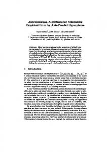
Figure 1.

Instances of MKAR.

N3DM, construct the following instance I 0 of MKAR. For each ai , bi , ci in N3DM, add items of weight ai , bi + d, ci + 2d, respectively, in I 0 . Add n knapsacks in I 0 with capacity 4d each. An item of weight ai can be assigned to knapsack i only, i = 1, . . . , n. The remaining items can be assigned to any knapsack (see figure 1(a)). Next, we add knapsacks n + 1, . . . , n + k, and items 1, . . . , k + 1, where k is an arbitrary positive integer. Each new knapsack has unit capacity. The first new item has weight 1/nd and can be assigned to knapsacks n and n + 1. Items 2 through k + 1 have unit weight. New knapsack n + i can only hold new items i and i + 1, for i = 1, . . . , k (see figure 1(b)). Note that the bipartite graph representation of I 0 is connected. It is easy to show that there exists a solution to N3DM if and only if there is an assignment of value 4nd + k for I 0 . A complete bipartite graph with the item and knapsack sets of I 0 has (3n + k + 1) ∗ (n + k) edges. On the other hand, in the bipartite graph representation of I 0 , there are 2n 2 + n + 2k + 1 edges. As k gets arbitrarily large (in particular, an order of magnitude larger than n), the edge density of the bigraph representation of I 0 will be O(2/k), which is the order of minimum density for a connected bigraph. Hence, there are very sparse instances of MKAR which are as hard as the N3DM problem. 2

3.

Maximizing assigned weight under assignment restrictions

In this section, we first show that solutions with a certain property, which we call the halffull property, are 1/3-approximations. We present a greedy algorithm framework which


175

produce solutions with the half-full property, i.e., the performance ratio of such algorithms is 1/3. We also show that this performance ratio is existentially tight. Next, we present two different algorithms both having performance ratio 1/2. The first algorithm solves m single knapsack problems and the second algorithm is based on rounding an optimum vertex solution of the LP relaxation. 3.1.

Greedy approaches

We first characterize a property common to the solutions generated by certain greedy approaches. Definition 3.1. A solution for MKAR has half-full property if the following condition holds: For every unassigned item in the solution, any knapsack to which this item is admissible is at least half full. We show that any solution with the half-full property has at least one third of the assigned weight of an optimum solution. Lemma 2.

Any solution with half-full property is a 1/3-approximation.

Proof: Consider a solution with the half-full property. Let U be the set of items not assigned to any knapsack and AU be the set of knapsacks eligible to accommodate at least one of the items in U , i.e., AU = ∪ j∈U A j . Let C(AU ) be the total capacity of the knapsacks in AU and W (AU ) be the total weight of the items assigned to the knapsacks in AU in the solution. Let W be the total assigned weight. By the half-full property, at least half of the capacity of any knapsack in AU is filled in the solution, i.e., C(AU ) ≤ 2W (AU ). In an arbitrary feasible solution, let U 0 ⊆ U be the set of items which are assigned to knapsacks and W (U 0 ) be the total weight of these items. In any solution, including the optimum solution, W (U 0 ) ≤ C(AU ) since items in U 0 are admissible only to knapsacks in AU . Thus, in any solution the maximum weight one could obtain by assigning items in U to the knapsacks is C(AU ). The total weight of the remaining items, i.e., the items in N − U , is W . Hence, W + C(AU ) is an upper bound on the total weight of any solution. 2 Since W + C(AU ) ≤ W + 2W (AU ) ≤ 3W , the result follows. Greedy algorithms based on the following framework generate solutions that have the half-full property. Algorithm Greedy Sort items by weight in non-increasing order. Sort knapsacks in any order. At each step, assign the next item in the list to the first eligible knapsack (if any) considering capacity and assignment restrictions. Theorem 3. Algorithm Greedy is a 1/3-approximation algorithm for MKAR.

176

DAWANDE ET AL.

Proof: The proof follows by showing that the solutions generated by algorithm Greedy have the half-full property. Consider a solution generated by algorithm Greedy. In that solution, let U be the set of items not assigned to any knapsack and AU be the set of knapsacks eligible to accommodate at least one of the items in U . Pick any item j ∈ U . All the knapsacks in A j (i.e., the knapsacks to which item j is admissible) must be (partially) filled; otherwise, item j would be assigned. Suppose there is a knapsack i ∈ A j , which has more than half of its capacity ci free. Since item j is unassigned, w j > ci /2, and by the greedy choice of the algorithms, there must be another item k with wk ≥ w j > ci /2, which has already been assigned to knapsack i and we have a contradiction. Note that if we sort the knapsacks in non-decreasing order of capacity in Algorithm Greedy, it is a 1/2-approximation algorithm for MKP with the objective of maximizing assigned weight, whereas its performance ratio is 1/3 for MKAR, which has assignment restrictions. The performance ratio 1/3 is tight, as shown by the following example. 2 Example 1. There are three items with weights M + ², M and M, and two knapsacks with capacities 2M and M + ², respectively. Item 1 could be assigned to either of the knapsacks whereas items 2 and 3 can only be assigned to knapsack 1. Algorithm Greedy would assign item 1 to knapsack 1 (no other assignments) with total assigned weight M + ². In the optimum solution, item 1 is assigned to knapsack 2 and items 2 and 3 are assigned to knapsack 1, with total weight 3M + ².

3.2.

Solving single knapsack problems

Consider an algorithm that runs through the knapsacks in any order and solves a single knapsack problem for each knapsack to find a maximum weight packing of admissible items. We will call such an algorithm a successive knapsack algorithm. The generic algorithm is as follows. Successive Knapsack Algorithm: Initialize: S = N , Weighti = 0, for i = 1, . . . , m. For each knapsack i, Solve a single knapsack problem for knapsack i with item set S ∩ Bi to maximize assigned weight. Let Si be the set of items packed with total weight Weighti . Remove Si from S. The algorithm requires the solution of m single knapsack problems, which can be solved in pseudo-polynomial time by dynamic programming. Theorem 4. Successive Knapsack Algorithm is a 1/2-approximation algorithm for MKAR. P Proof: Let AW denote the total weight assigned by the algorithm, i.e., AW = i∈M Weighti . Let S be the set of items remaining unassigned at the end of the algorithm. The


177

proof follows from the following claim. In any feasible solution to MKAR, the total weight of items from S that are assigned is at most AW. To prove this claim consider any feasible solution x. Suppose the weight of items in S that are assigned in this solution equals AW +² for some ² > 0. Then in solution x, there is at least one knapsack, say i, with weight greater than Weighti assigned to it from S. However, this is a contradiction because when we filled knapsack i in the algorithm, we used an item set including S, and chose a maximum weight assignment of value Weighti . Thus, any feasible solution can have total assigned weight at most 2AW. 2 Note that instead of solving the single knapsack problems exactly, we can obtain 1/(1 + ²)approximate solutions for any ² > 0 by a FPTAS (Ibarra and Kim, 1975). In this way, it is easy to check that, for any ² > 0, we can get a 1/(2 + ²)-approximate solution to MKAR in time polynomial in the instance size and in 1/². To see this, we can weaken the claim in the above proof to argue that in any feasible solution, the total weight of items from S that are assigned is at most (1 + ²) AW. Suppose this were not true—then as above, there exists a knapsack whose weight from S in the solution x is greater than (1 + ²)Weighti , a contradiction to the guarantee of the FPTAS used to solve the single knapsack problem. The performance guarantee in the above theorem can be achieved as demonstrated by the following example: We have two knapsacks with capacity 2M each, and two items with weights M and M + ² respectively. While the heavier item can be assigned to both knapsacks, the other can be assigned to only one of them. The optimal solution can obviously assign both items but if the knapsack that can accept both items is chosen first in the above algorithm, the heavier item is assigned to it leaving the other unassigned.

3.3.

LP rounding: A

1 2

approximation algorithm

The IP formulation of the MKAR problem is as follows: max

P P

w j xi j

i∈M j∈Bi

st

P

w j xi j ≤ ci , i ∈ M

j∈Bi

P

xi j ≤ 1, j ∈ N

i∈A j

xi j ∈ {0, 1}, i ∈ A j , j ∈ N

where the 0-1 variable xi j denotes whether item j is assigned to knapsack i. Let us denote the LP relaxation by LP-MKAR, which is obtained by replacing the constraints xi j ∈ {0, 1} with the constraints 0 ≤ xi j ≤ 1. LP-MKAR can be solved by a maximum flow algorithm on a directed graph constructed from the bigraph G as follows. Each edge ( j, i) of G is directed from the item node j to the knapsack node i and is assigned capacity w j . A source node s is connected to each item node j via an arc (s, j) with capacity w j . In addition, a sink node t is connected to each knapsack node i via an arc (i, t) with capacity ci . Then, the maximum flow from s to

178

DAWANDE ET AL.

t equals the LP relaxation value and the amount of flow on arc ( j, i) divided by w j gives the value of x ij . Thus, if flow on ( j, i) equals w j , i.e., xi j = 1, then item j is assigned to knapsack i. If 0 < xij < 1, the variable is said to be fractional (in the corresponding solution). Let x be an optimal basic feasible solution to LP-MKAR and let f denote the vector of fractional variables of x. We denote the subgraph of the bigraph representation G induced by the edges in f by RG and call it the residual graph. Lemma 5.

The residual graph, RG , of the LP relaxation is a forest.

Proof: Suppose RG contains a cycle, say C. N ote that C has to be even. Let C = I1 , K 1 , I2 , K 2 , . . . , K l , I1 , where I j are item nodes (with weight w j ) and K i are knapsack nodes in the cycle. Let f C = ( f 1 , . . . , f k ) denote the vector of fractional values on the edges of C, when C is traversed in the above order. Keeping all other values fixed, we can perturb the variables on this cycle such that x is a convex combination of two feasible solutions, which is a contradiction. The two feasible solutions x 1 and x 2 are obtained by adding the vectors f 1 and f 2 to f C , respectively. The first perturbation vector is f 1 = 1 1 1 1 ε, w ε, − w ε, w ε, . . . , −ε) for some suitable ² > 0 and the second one is f 2 = (ε, − w w2 w2 w3 w3 1 1 − f . The solutions x and x 2 are feasible to LP-MKAR since the perturbations preserve both the capacity and the assignment constraints. In addition, x is a convex combination of 2 x 1 and x 2 since x = 12 (x 1 + x 2 ). We can consider each connected component of RG separately. Let OPT denote the optimum value of LP-MKAR and let AW(K i ) denote the total weight assigned to knapsack K i in x. In RG , if a knapsack has degree 1, then we refer to that knapsack as a singleton knapsack. Lemma 6. If RG has a singleton knapsack node, say K 1 , then there is a rounding step for knapsack K 1 such that R1 ≥ OPT − 12 AW(K 1 ), where R1 denotes the objective function value of the solution obtained after the rounding step. Proof of Lemma 6: Let S denote the set of items which have been assigned (integrally) to knapsack K 1 by the solution x. Note that S is nonempty, otherwise there would be no fractional variable incident on K 1 . Let W (S) denote the total weight of items in S. In addition, let I1 be the item which is fractionally assigned to knapsack K 1 with value f 1 . If W (S) ≥ w1 f 1 , then we round f 1 down to zero. Now K 1 has no fractional variable incident on it. Let us denote the new solution by x1 . Then, x1 has objective value R1 = OPT −w1 f 1 . Since AW(K 1 ) = w1 f 1 +W (S) ≥ 2w1 f 1 , it is true that R1 ≥ OPT − 12 AW(K 1 ). On the other hand, if w1 f 1 > W (S), then we unassign all items in S and round f 1 to 1. We also round all other fractional variables incident on I1 to 0. Then, R1 ≥ OPT −W (S) ≥ OPT − 12 AW(K 1 ). 2 Note that after the rounding step for knapsack K 1 , node K 1 is removed from RG and the new residual graph is still a forest, as the rounding step does not add any new edges to RG . We call the above rounding step a “type 1” step.


179

Next we define a second type of rounding step: a “type 2” step. Lemma 7. If RG has no singleton knapsack node, then the fractional solution corresponding to RG can be perturbed such that (i) the objective function value does not change and (ii) the number of arcs in RG reduces by at least 1. Proof of Lemma 7: Suppose there exists no singleton knapsack at the current bigraph RG . Consider a knapsack node K of degree at least 2. Let e1 and e2 be two edges incident on K . Let P1 and P2 be the two maximal paths originating from node K and starting with edges e1 and e2 , respectively. These paths must be disjoint since RG has no cycles. Each of these paths must have an item node as its endpoint, for otherwise, we would have a singleton knapsack node. The key observation is that for any of these paths, the leaf node has an assignment constraint which is not tight. Along each path we can perturb the solution such that we obtain a feasible solution having one less fractional variable and the same objective value. The perturbations are as follows. Let f 1 = ( f 1 , . . . , f k ) denote the vector of fractional values on the edges of P1 and let I1 , . . . , Ik be the item nodes of P1 . Similarly, let f 2 = ( f k+1 , . . . , f p ) denote the fractional vector and Ik+1 , . . . , I p denote the items of P2 . We modify the current solution x in f 1 and f 2 by adding the vectors f ε1 and f ε2 , k k k k ε, − w ε, w ε, . . . , − wwk−1 ε, ε) and respectively. The first perturbation vector is f ε1 = ( w w1 w1 w wk wk wk wk wk 2 2 the second one is f ε = (− wk+1 ε, wk+1 ε, − wk+2 ε, . . . , w p−1 ε, − w p ε). (See figure 2). Note that the new solution is feasible to LP-MKAR since the perturbations preserve both the capacity and the assignment constraints. Now we can increase ε until one of the fractional

Figure 2.

Perturbation of the fractional variables.

180

DAWANDE ET AL.

values hits 0 or 1. This new solution will have at least one less fractional variable. Thus, at least one edge is removed from RG . It is easy to check that the perturbations do not change the objective function value. Therefore, a new feasible solution with the same objective value is obtained. 2 Now using the two types of rounding steps, we have the following rounding scheme. LP Rounding Algorithm: Step 0: Obtain a vertex solution x to the LP-MKAR. Construct the residual graph RG based on the fractional variables. Step 1: If there exists a singleton knapsack node in RG , perform a type 1 rounding. Update RG . Repeat Step 1 until there are no singleton knapsacks in RG . Step 2: Pick a knapsack node, say K, of degree at least 2. Perform a type 2 rounding. Update RG . Go to Step 1. Theorem 8. LP Rounding Algorithm is a 1/2-approximation algorithm for MKAR. Proof: After every type 1 rounding step, a knapsack node and an edge incident on it are removed from RG . After every type 2 rounding step, at least one edge is removed from RG . Since RG has at most m + n edges, the rounding algorithm has at most m + n iterations each of which takes at most O(m + n) time. The LP relaxation can be solved by a maximum flow algorithm and a vertex solution can be found in polynomial time (Ahuja et al., 1993). After any type 2 step, the objective value does not change (Lemma 7). Let Rk denote the objective function value after kth type 1 step. Suppose we pick Pkknapsack K i at the AW(K i )). Let p ith type 1 step. Then, due to Lemma 6 we have Rk ≥ OPT − 12 ( i=1 denote the last type 1 step. Note that p ≤ m. Then, Ã p ! 1 1 X 1 R p ≥ OPT − AW(K i ) ≥ OPT − OPT = OPT. 2 i=1 2 2 Hence, the feasible integral solution output by the algorithm has objective value at least half of the LP relaxation value. 2 Corollary 9. The LP-IP integrality gap for MKAR is 2. That is, the optimal objective value of the LP relaxation for the MKAR is at most 2 times the optimal objective value of MKAR. Proof of Corollary 9: Given an instance I of MKAR, let L P(I ) denote the optimal value for the LP relaxation, and let OPT(I ) denote the optimal value for MKAR. In addition, let H (I ) denote the value of the solution output by the rounding algorithm for instance I . By the proof of Theorem 8, 12 LP(I ) ≤ H (I ). Since H (I ) ≤ OPT(I ), it follows that LP(I ) ≤ 2OPT(I ), for any instance I . 2


181

The IP-LP gap of 2 is tight, as shown by the following simple instance. Consider the instance with one knapsack of capacity 2M, and only 2 items of weight M + ² and M. The optimum IP solution has assigned weight M + ², whereas optimum value of the LP relaxation is 2M. The approximation ratio of 2 is also tight as seen from the following example: Consider the instance with one knapsack of capacity 2M, and 3 items with weights w1 = 1, w2 = M, w3 = M. An optimal basic solution to the LP relaxation is x1 = 1, x2 = 1 . The LP rounding algorithm produces the solution x1 = 1, x2 = 1, x3 = 0 of and x3 = M−1 M value M + 1 while the optimal solution is of value 2M. Remark. Chekuri (1999) has pointed out to us that the above LP-rounding result can also be derived from a similar rounding result for the generalized assignment problem by Shmoys and Tardos (1993). In the generalized assignment problem, jobs are assigned to machines. For each job i and machine j, there are two positive parameters: c(i, j), the cost of assigning i to j and s(i, j), the size of i if assigned to j. Each machine also has a capacity b( j). The objective is to assign jobs such that capacity constraints are not violated and the total cost of the assignment is minimum. Shmoys and Tardos (1993) show how to round the natural LP relaxation to obtain a solution with the following properties. 1. The cost of the rounded solution is no more than cost of the LP solution. 2. If a machine’s capacity is violated in the rounded solution, then there is one job assigned to the machine whose removal results in satisfying the capacity constraint for the machine. Furthermore, this job was assigned fractionally to this machine in the LP solution. One can use the above facts to obtain a 12 -approximation for our problem as follows. The machines correspond to knapsacks and jobs to items. First add an extra machine with zero weight (profit) for all items and with sufficient capacity to pack all items to it. Next, we convert the weights (profits) to costs by subtracting them from a sufficiently large number. Finally, we handle the assignment restrictions by giving very high costs (higher than the large number used in the previous step) to infeasible assignments. This creates a feasible instance of the generalized assignment problem and the minimum cost of an optimal assignment for this instance can be mapped to one with maximum assigned weight for the original MKAR problem. Consider the rounded solution from the techniques of (Shmoys and Tardos, 1993). From (1) above, this solution has the minimum cost and hence the maximum assigned weight. However it is not a feasible solution as per (2). But we can obtain a feasible solution by discarding, for each violated machine (knapsack), either the job (item) whose removal ensures that capacity constraint is not violated, or the rest of the items, whichever has smaller total weight. One of these sets has at least half the total weight giving a feasible rounded solution with at least half the weight of the LP solution. 4.

The bicriteria problem

In the surplus inventory matching application that motivated our study of the MKAR problem, in addition to maximizing assigned weight, minimizing total utilized capacity (or

182

DAWANDE ET AL.

equivalently, total unused capacity of the utilized knapsacks) is also an important objective that needs to be considered. With the two objectives, the choice of the knapsack to which an item is assigned becomes more critical. As the problem gets sparser, any solution that maximizes assigned weight does not necessarily utilize small capacity. In approximating a bicriteria problem, it is common practice to choose one of the criteria as the objective and to bound the value of the other by means of a constraint. In this section, we consider BMKAR with the objective of minimizing total utilized capacity (total capacity of all the bins that are at least partially filled), subject to a lower bound T on the assigned weight. It is easy to construct an instance of this capacity minimization problem (CM) for which the algorithms we have presented so far fail to perform well in terms of minimizing utilized capacity. One natural question to ask is: what is the best possible performance guarantee of an algorithm for the objective of minimizing utilized capacity, if the weight constraint must be satisfied exactly? The following theorem shows that the best possible performance ratio for any polynomial time algorithm is log n. Theorem 10. Any algorithm which satisfies the assigned weight constraint cannot have a performance ratio better than log n (where n is the number of items) for BMKAR with the objective of minimizing utilized capacity, unless unless P = NP. Proof of Theorem 10: The reduction is from the minimum set cover. Given an instance of the minimum set cover, i.e., a set S, with |S| = n and a collection of subsets C1 , C2 , . . . , Ck of S, construct an instance of BMKAR as follows. For each element of S, create an item of weight 1/n. For each subset Ci , create a knapsack with capacity 1. Items corresponding to elements of Ci are admissible to this knapsack. Let the minimum weight we want to assign equal T = 1. The minimum capacity needed to assign weight 1 is equal to the minimum number of knapsacks to assign all items, which is equal to the cardinality of the minimum set cover. However, minimum set cover is not approximable within (1 − ²) log n for any ² > 0 unless P = NP (Arora and Sudan, 1997; Raz and Safra, 1997; Feige, 1996). 2 In this section, we present an algorithm, which relaxes the assigned weight constraint in order to minimize the utilized capacity. An (α, β)-approximation algorithm for CR generates solutions with utilized capacity at most β times the optimum capacity and with assigned weight at least α times the lower bound T , where β ≥ 1 and 0 < α ≤ 1. The algorithm we present is a (1/3, 2)-approximation algorithm. 4.1.

Solving single knapsack problems

We use the successive knapsack algorithm of Subsection 3.2 with a specific minimum ratio rule to select the next knapsack. Given a set S ⊆ N of items, let Weighti denote the maximum weight of items from S that can be packed into knapsack i. Note that Weighti can be found by a pseudo-polynomial algorithm that solves a single knapsack problem (or can be approximated by a FPTAS). Let


183

us denote the unused capacity, or waste, in this knapsack by Wastei = ci − Weighti . Let AW denote the total assigned weight by the following algorithm. Selective Successive Knapsack (SSK) Algorithm: Initialize: S = N , R = M, Weighti = 0, i ∈ M, AW = 0. (1) For all i ∈ R, calculate Weighti and Wastei by solving a single knapsack problem for knapsack i with item set S ∩ Bi . (2) Pick the knapsack with minimum ratio of Wastei /Weighti , say knapsack k. (3) Pack items into knapsack k to obtain Weightk , add Weightk to AW . (4) If AW ≥ T /3, then terminate the algorithm. (5) Otherwise, (5.1) Remove assigned items from S and knapsack k from R. (5.2) If R is nonempty, go to Step (1). (5.3) If R is empty, terminate the algorithm. If the SSK algorithm ends with AW < T /3, then by the following argument we can conclude that there exists no assignment of weight at least T for CM. Since the algorithm is a successive knapsack algorithm, by Theorem 4, we should be able to assign at least T /2, if there is any feasible solution with assigned weight T or more. In order to bound the capacity of the last knapsack picked, we run the algorithm at most m different times as follows: In the kth run, we exclude the k − 1 knapsacks with the largest capacities. Of course, we stop the runs when AW gets smaller than T /3 in a particular run. Among the solutions output over all runs, the one with minimum capacity is picked. Theorem 11. If the CM problem is feasible, a (1/3, 2)-approximate solution is obtained by running the selective successive knapsack algorithm at most m times. Proof: Suppose the problem is feasible. Consider the run in which the maximum capacity knapsack allowed is the maximum capacity knapsack in an optimal solution. Note that the solution of this run has AW at least T /3 (by Theorem 4). We bound the utilized capacity for this run by twice that of the optimal solution. Since we pick the minimum capacity solution over all runs, the performance ratio on the capacity follows. Consider a solution x H output by the algorithm and an optimal solution xOPT . Modify x OPT to obtain solution xOPT 0 as follows. Let OPT be the set of knapsacks used by the optimal solution. Let H be the set of knapsacks, excluding the last one picked, by the algorithm. Remove from OPT all knapsacks that are also in H . Denote the knapsacks in OPT − H by OPT 0 . Among items assigned to remaining knapsacks of OPT, unassign those assigned to H in x H . Claim 1: The weight of items removed from OPT is at most 2T /3. Proof of Claim 1: Let W H denote the weight assigned to H in x H . Clearly, weight of items assigned in both x H and xOPT is at most W H . Let S be the set of items that are assigned to a knapsack in H ∩ OPT in xOPT but are not assigned anywhere in x H . We need to bound

184

DAWANDE ET AL.

the weight of S. Let Si be the items from S assigned to knapsack i ∈ H in xOPT . These items were available when knapsack i was filled by the algorithm. Therefore, weight of Si can be at most Weighti . Thus, weight of S is at most W H . By the stopping condition, 2 W H < T /3. Hence, total weight removed from OPT is at most 2W H < 2T /3. P For a knapsack subset I , let C(I ) denote i∈I ci . For a solution x, let AW(x) denote total weight assigned in x and Waste(x) denote the total waste in x. The following are true. 1) C(OPT 0 ) ≤ C(OPT) since OPT 0 ⊆ OPT. 2) AW(xOPT 0 ) ≥ T /3 because of Claim 1 and AW(xOPT ) ≥ T . 3) Waste(xOPT 0 ) + T /3 ≤ C(OPT 0 ) by the definition of Waste and 2). For any knapsack i ∈ H , Waste(xOPT 0 ) Waste(xOPT 0 ) Wastei ≤ . ≤ Weighti AW(xOPT 0 ) T /3 The first inequality follows since the ratio of a knapsack picked by the algorithm is smaller than the ratio of any other remaining knapsack, where the ratios depend on the items available at the time of the choice. That is, when the heuristic picks knapsack i, knapsacks in OPT 0 have larger ratios than that of i. However, in the solution xOPT 0 , some of the items have been unassigned, thereby making the ratios of knapsacks in OPT 0 even larger. The second inequality follows directly from 2). By summing these inequalities multiplied by Weighti over i’s, we obtain X

Wastei ≤

i∈H

Since

P i∈H

X

Waste(xOPT 0 ) X Weighti . T /3 i∈H

Weighti ≤ T /3,

Wastei ≤ Waste(xOPT 0 ).

i∈H

Using this inequality together with 1) and 3), we get X X Wastei + Weighti ≤ Waste(xOPT 0 ) + T /3 ≤ C(OPT 0 ) ≤ C(OPT). C(H ) = i∈H

i∈H

We can also bound the capacity of the last knapsack picked by C(OPT) by our choice of the run we are analyzing. 2 As in the proof of Theorem 4, using a FPTAS instead of an exact algorithm to solve the 1 , 2). single knapsack problems results in a performance guarantee of ( 3+²


5.

185

Conclusions

In this paper, we generalized the classical multiple knapsack problem by allowing assignment restrictions. For the objective of maximizing assigned weight, we presented a 1/3approximation algorithm and two 1/2-approximation algorithms. Whether a performance ratio better than 1/2 can be achieved is an interesting open question. For the bicriteria problem, where we consider minimizing utilized capacity as well as maximizing assigned weight, we give a (1/3, 2)-approximation algorithm. Again, it would be interesting to improve the performance ratio for this problem. Notes 1. The author was a post-doctoral fellow at IBM T.J. Watson Research Center when most of this research was conducted. 2. The author was an intern at IBM T.J. Watson Research Center when most of this research was conducted.

References A.K. Ahuja, T.L. Magnanti, and J.B. Orlin, Network Flows, Prentice Hall: New Jersey, 1993. S. Arora and M. Sudan, “Improved low degree testing and its applications,” in Proc. 29th ACM Annual Symp. on Theory of Computing, 1997, pp. 485–495. A. Caprara, H. Kellerer, and U. Pferschy, “The multiple subset sum problem,” Technical Report 12/1998, Faculty of Economics, University of Graz, 1998. C. Chekuri, Personal communication, July 1999. E.G. Coffman, M.R. Garey, and D.S. Johnson, “Approximation algorithms for bin-packing: An updated survey,” in Algorithm Design for Computer System Design, G. Ausiello, M. Lucertini, and P. Serafini (Eds.), SpringerVerlag: Vienna, 1984, pp. 49–106. E.G. Coffman, M.R. Garey, and D.S. Johnson, “Approximation algorithms for bin-packing: A survey,” in Approximation Algorithms for NP-hard Problems, D.S. Hochbaum (Ed.), PWS Publishing Company: Boston, 1997, pp. 46–93. M.W. Dawande and J.R. Kalagnanam, “The multiple knapsack problem with color constraints,” Technical Report, RC21138, IBM T.J. Watson Research Center, Yorktown Heights, NY, 1998. U. Feige, “A threshold of ln n for approximating set cover,” in Proc. 28th Annual ACM Symposium on Theory of Computing, 1996, pp. 314–318. C.E. Ferreira, A. Martin, and R. Weismantel, “Solving multiple knapsack problems by cutting planes,” SIAM J. Optimization, vol. 6, no. 3, pp. 858–877, 1996. D.K. Friesen and M.A. Langston, “Variable sized bin packing,” SIAM J. Computing, vol. 15, pp. 222–230, 1986. M.R. Garey and D.S. Johnson, Computers and Intractability: A Guide to the Theory of NP-Completeness, W.H. Freeman and Co.: San Francisco, 1979. M.S. Hung and J.C. Fisk, “An algorithm for 0-1 multiple knapsack problems,” Naval Res. Logist. Quarterly, vol. 24, pp. 571–579, 1978. O.H. Ibarra and C.E. Kim, “Fast approximation for the knapsack and sum of subset problems,” J. ACM, vol. 22, pp. 463–468, 1975. J. Kalagnanam, M. Dawande, M. Trumbo, and H.S. Lee, “The surplus inventory matching problem in the process industry,” Technical Report RC21071, IBM T.J. Watson Research Center, Yorktown Heights, NY, 1997. V. Kann, “Maximum bounded 3-dimensional matching is MAX SNP-complete,” Information Process. Lett., vol. 37, pp. 27–35, 1991. R.M. Karp, “Reducibility among combinatorial problems,” in Complexity of Computer Computations, R.E. Miller and J.W. Thatcher (Eds.), Plenum Press: New York, 1972, pp. 85–103.

186

DAWANDE ET AL.

S. Martello and P. Toth, “Solution of the zero-one multiple knapsack problem,” Euro. J. Oper. Res., vol. 4, pp. 322–329, 1980. S. Martello and P. Toth, “A bound and bound algorithm for the zero-one multiple knapsack problem,” Discrete Applied Math., vol. 3, pp. 275–288, 1981a. S. Martello and P. Toth, “Heuristic algorithms for the multiple knapsack problem,” Computing, vol. 27, pp. 93–112, 1981b. S. Martello and P. Toth, Knapsack Problems, John Wiley and Sons, Ltd.: New York, 1990a. S. Martello and P. Toth, “Lower bounds and reduction procedures for the bin packing problem,” Discrete Applied Math., vol. 28, pp. 59–70, 1990b. R. Raz and S. Safra, “A sub-constant error-probability low-degree test, and a sub-constant error-probability pcp characterization of NP,” in Proc. 29th Annual ACM Symp. on Theory of Computing, 1997, pp. 314–318. D. Shmoys and E. Tardos, “An approximation algorithm for the generalized assignment problem,” Math. Programming, vol. 62, pp. 461–474, 1993.