2011 American Control Conference on O'Farrell Street, San Francisco, CA, USA June 29 - July 01, 2011
Approximation Algorithms for a Heterogeneous Multiple Depot Hamiltonian Path Problem S. Yadlapalli, Jungyun Bae, S. Rathinam, and S. Darbha Abstract— In this article, we present the first approximation algorithm for a routing problem that is frequently encountered in the motion planning of Unmanned Vehicles (UVs). The considered problem is a variant of a Multiple Depot-Terminal Hamiltonian Path Problem and is stated as follows: There is a collection of m UVs equipped with different sensors on-board and there are n targets to be visited by them collectively. There are restrictions on the targets of the following type: (1) A target may be visited by any UV, (2) a target must be visited only by a subset of UVs (with appropriate on-board sensor) and (3) a target may not be visited by a subset of UVs (as the set of onboard sensors on the UV may not be suitable for viewing the targets). The UVs are otherwise identical from the viewpoint of dynamic constraints on their motion and hence, the cost of traveling from a target A to a target B is the same for all vehicles. We will assume that triangle inequality is satisfied by the cost associated with travel, i.e., it is cheaper to travel from a target A to a target B directly than to go via an intermediate target C. The UVs may possibly start from different locations (referred to as depots) and are not required to return to the depot. While there are different objectives that can be considered for this problem, we consider the total cost of travel of all the UVs as an objective to be minimized. The problem considered in this article is a generalized version of single depot-terminal Hamiltonian Path Problem and is NP-hard.
I. I NTRODUCTION Surveillance applications involving Unmanned Vehicles (UVs) require different UVs with different capabilities to gather information about a set of targets. Information is often gathered about the targets by an appropriate UV visiting a target and gathering information about the target using its on-board sensors. Associated with the task of information gathering is the problem of routing UVs in some optimal manner and it is in connection with the routing, we address the following problem: There are m UVs that must collectively visit n targets. We assume that the vehicles are identical dynamically and hence, the cost of traveling from any target A to any other target B with identical headings is the same for every UV in the collection. The UVs differ from each other in their sensing capabilities and accordingly, we categorize the targets into three disjoint subsets: 1) Category I: Subset of targets which can be visited by any UV. Graduate Student, Department of Mechanical Engineering, Texas A&M University, College Station, TX-77843-3123. Graduate Student, Department of Mechanical Engineering, Texas A&M University, College Station, TX-77843-3123. Assistant Professor, Department of Mechanical Engineering, Texas A&M University, College Station, TX-77843-3123. Professor, Department of Mechanical Engineering, Texas A&M University, College Station, TX 77843-3123,
[email protected]
978-1-4577-0079-8/11/$26.00 ©2011 AACC
2) Category II: Subset of targets that can be visited only by a specific UV or a subset of UVs. This arises in a scenario where the technology/equipment to accomplish the desired task on a target is available only to a subset of UVs. Also, if a group of targets form a cluster i.e., they are very close to each other in terms of distance, it might be economical to let one UV perform all the tasks on these group of targets. 3) Category III: Subset of targets that are unsuitable to be visited by a particular UV or a subset of UVs. Even though the cost of traveling from one target to another is the same for every UV, these restrictions on the assignment of UVs to target, which we will refer to as assignment constraints, introduce heterogeneity. The problem considered in this article is as follows: Given a set of depots (starting locations of UVs) and their corresponding terminals (ending locations of UVs) find a path for each vehicle such that • the path of each UV starts from its respective depot and ends at the corresponding terminal, • each target is visited exactly once by some vehicle, • the assignment constraints are satisfied and, • the total cost of the paths of all the UVs is a minimum. There are several applications ([1],[4],[11],[7], [6],[8]) where routing problems such as the one considered in this article arise. The problem considered in this article is a generalization of the Hamiltonian Path Problem (HPP) and its closely related Traveling Salesman Problem (TSP) and is NP-Hard. The generalizations of the HPP and TSP have received significant attention in the field of Combinatorial Optimization ([10],[9],[12],[3]). Because the problem is NPhard, one may not expect to find an optimal solution with a running time guarantee that is polynomial in the size of the problem. In this article, we will focus on approximation algorithms, which are polynomial time algorithms but relax the requirement of optimality; however, they provide bounds on the deviation of the cost of the suboptimal solution from the optimal cost without ever computing the optimal cost. An α −approximation algorithm [12] is an algorithm that • has a polynomial-time running time, and • returns a solution whose cost is within α times the optimal cost. We will assume that the cost of traveling from an origin to a target directly for each vehicle is no more expensive
2789
than the cost of traveling from the same origin to the target through an intermediate location. We say that the costs satisfy the triangle inequality if they satisfy the above property. It is known that there cannot exist a constant factor approximation algorithm for a HPP or a TSP if the triangle inequality is not satisfied unless P = NP. For this reason, we henceforth assume that this property holds for the cost associated with travel for every UV. There are a few approximation algorithms that are available for the variants of the TSP and the HPP. The symmetric TSP has two well known approximation algorithms - the 2 approximation algorithm obtained by doubling the minimum spanning tree (MST) and the 1.5 approximation algorithm of Christofides obtained through the construction of MST and a minimum perfect matching of vertices of MST with odd degree [2]. The best approximation algorithm currently available for the single HPP (a path that contains each vertex exactly once of minimum total cost) was proposed by Hoogeveen [3]. In [3], he proposed an approximation algorithm for three variants of single HPP that depend on the choice of the endpoints of the path. Hoogeveen modified the Christofides algorithm, and provided a 32 −approximation algorithm for the variant of the HPP problem when at most one endpoint is fixed and proposed a 35 −approximation algorithm when both endpoints are fixed. Rathinam et al. have provided 2−approximation algorithms for variants of the homogenous, multiple TSP and HPP in ([7],[6],[5]). A 32 −approximation algorithm was also developed for two variants of a 2-depot Hamiltonian path problem in [8] when the the costs are symmetric and satisfy the triangle inequality. In this article, we present a 11 3 -approximation algorithm for the multiple depot-terminal HPP with functional heterogeneity constraints. In the special case when the locations of the terminals coincides with their respective depots, the approximation factor of the proposed algorithm reduces to 3.5. This approximation factor of 3.5 also holds true for other variants of the heterogenous, multiple depot HPP when at most one endpoint is specified for each vehicle. II. P ROBLEM F ORMULATION Let the set of vertices D and T represent all the distinct depots and terminals respectively. Let |D| = |T |. Assume that there is an UV initially located at each of the depots. For every depot, di ∈ D, let there exist exactly one terminal vertex denoted by ti ∈ T . We require that each UV starting at its depot end its path at its corresponding (fixed) terminal. Let p := |D| denote the total number of depots. We first consider all the targets belonging to categories in I and II. We assume that all the targets are distinct, i.e.,
there are no two targets present at the same location. Let the set of targets which can be only visited by the ith UV that starts at di ∈ D be represented by Ai . Let us define A = A1 ∪ A2 ... ∪ A p . We assume that all the Ai ’s are disjoint, i.e., A1 ∩ A2 ... ∩ A p = φ . Let the common set of targets which can be reached by all UVs be F. S
S S
Define a graph (V, E) with V = D T A F denoting the set of all the vertices and E := V ×V denoting the set of all the edges joining any two vertices in V . Let c(Vi ,V j ) or simply ci j represent the cost of traveling from vertex Vi to vertex V j for all Vi ,V j ∈ V . We further assume that the costs are positive, symmetric and satisfy the triangle inequality, i.e., for all Vi ,V j ,Vk ∈ V and i 6= j 6= k, Ci j +C jk ≥ Cik . The symmetry of costs may not hold true for all UVs in general; however, by relaxing motion constraints, we assume that one can obtain symmetry in the cost of travel between any two targets. This is especially so when the constraint associated with forward travel in a Dubins’ vehicle is relaxed, one gets a Reed-Shepp vehicle and the costs are symmetric. While such a relaxation may not solve the original problem, it serves two purposes: firstly, it provides a lower bound for the optimal solution, and secondly, if the distances between targets is sufficiently large compared to the turning radius as in the case of Dubins’ vehicle, the asymmetry in the cost is not so significant compared to the Euclidean distance between the targets. In such circumstances, the proposed approximation algorithms provide “adequate” feasible solutions.
A path for a UV is a sequence of vertices visited by the vehicle. The first vertex is called the start vertex and the last vertex in the sequence is called the end vertex. A path with no repeated vertices is called a simple path. In this work, we refer simple paths as simply paths. However, it should be noted that since the costs satisfy triangle inequality, it is always possible to shortcut a repeated vertex and obtain another path of lower cost spanning (or visiting) all the vertices.
A path travelled by the ith UV is an ordered set, PAT Hi , and can be represented by the form {di ,Vi1 , .....,Vir ,ti }, S where Vil ∈ A F, l = 1, ...., r corresponds to the r distinct targets being visited in that sequence by the ith UV. These set of targets being visited by the ith UV must include the set Ai (which can be only visited by ith UV and subset (could be empty) of common targets, F. The cost of traveling PAT Hi is defined as C(PAT Hi ) = cdi i1 + ∑ j=r−1 j=1 cik ik+1 + cir ti . The Combinatorial Motion planning Problem (CMP) addressed in this article is to find a PAT Hi for the ith UV (i = 1, · · · , p) such that each target is visited exactly once, all the assignment constraints are satisfied and the total cost defined by ∑i=p i=1 C(PAT Hi ) is minimized.
2790
i=p all the targets in Ai and Fi . Let P = ∪i=1 Pi . Since P is a collection of edge-disjoint simple paths and satisfies all the constraints, P is a feasible solution to CMP.
III. A PPROXIMATION A LGORITHM FOR THE CMP Here, we present an algorithm, Approxcmp , which constructs a feasible solution to the CMP. We later prove that this algorithm produces a solution with an approximation factor of 11 3 . Approxcmp is as follows: 1) For each i ∈ 1, · · · , p, do the following: • Consider the subset of vertices Si = {di } ∪ Ai ∪ {ti } ∀i = {1.....p}, where di and ti are the depot and terminal vertices corresponding to the ith UV. Compute a feasible depot-terminal path, HPPi , that starts from di and ends at ti using the Hoogeveen’s algorithm [3]. Let EHPPi be the set of all the edges present in HPPi . Sp Let EHPP = i=1 EHPPi . Let the total cost of these i=p C(HPPi ) . paths be denoted by CHPP = ∑i=1 2) In this step we distribute the common targets, F, among all the UVs. After the distribution, we will construct a tour for each UV that starts at its depot and visits its assigned set of common targets. The algorithm for distributing the common targets among the UVs is as follows: Consider the set M = D ∪ F. Assign zero costs to all the edges among the depots. For the rest of edges retain the costs assigned earlier. Now, construct a Minimum Spanning Tree (MST) on M with the assigned costs using Kruskal’s algorithm. Truncate all the zero cost edges (among depots) in the resultant MST. This results in a forest with exactly p connected components. Each of the connected component has exactly one depot in it. (This follows from the fact that, during each iteration, the Kruskal’s algorithm adds a (non-used) cheapest, cost edge to the solution such that no cycle is formed among all the added edges in the solution. Therefore, there are exactly |p − 1| zero cost edges joining the p depots in the solution.) Let EF be the set of the remaining edges after removing all the zero cost edges from the MST. EF corresponds to a forest with p trees where each tree contains one depot. Also, let EFi be the set of edges present in the ith tree. 3) Double the edges of EFi . Since EFi is a tree, doubling the edges of EFi would result in a connected, Eulerian graph. Therefore, one can find an tour (TFi ) by shortcutting the edges in the Eulerian tour. The cost of this tour must be at most twice the cost of the edges in EFi since the costs satisfy the triangle inequality. 4) Consider the set of edges denoted in TFi ∪ HPPi . By construction, there are exactly three edges incident on di where one belongs to the path HPPi and two belong to the tour, TFi . By shortcutting an edge from TFi and an edge that belongs to HPPi one can form a path Pi that starts from depot di , ends at terminal ti and visits
The following theorem establishes the approximation ratio of the above algorithm. Theorem 1. The approximation factor of Approxcmp is
11 3 .
Proof. First, we will prove that the running time of Approxcmp is a polynomial function of the number of targets and depots. The number of steps required by Approxcmp is dominated by the computations in steps 1 and 2 of the algorithm. Step 1 of Approxcmp uses the Hoogeveen algorithm which requires O(m3 ) steps where m is the total number of targets. Step 2 of Approxcmp uses the Kruskal’s algorithm which requires O((m + p)2 log(m + p)) steps to compute. Therefore, the running time of Approxcmp is a polynomial function of the number of targets and depots. Now, we will prove the guarantee on the quality of the solutions. Let OPT denote an optimal solution to the CMP and let COPT denote its corresponding cost. Let the optimal path corresponding to the UV at depot di in OPT be OPT i . We will now bound the costs of all the HPP’s found in step 1 of Approxcmp . Consider the Single Depot-Terminal HPP restricted to the set Si = {di } ∪ Ai ∪ {ti }. Let HPPi∗ be an optimal solution to this problem. Note that the HPPi found in step 1 of Approxcmp is a feasible solution to the single Depot-Terminal HPP on Si . Also note that the path OPT i visits each target in Si in addition to some common targets from F. Since the costs satisfy the triangle inequality, by shortcutting all the common vertices in OPT i that do not belong to Si , one can easily conclude that: 3 COPT i ≥ CHPPi∗ ≥ CHPPi . 5
(1)
The latter part of the above inequality follows from Hoogeveen’s result for Single Depot-Terminal HPP. Summing the above result for all the vehicles, we get, 5 COPT ≥ CHPP . 3
(2)
In the following discussion, we will bound the costs of all the tours found in steps 2 and 3 of Approxcmp . Note that the optimal path OPT i visits some common vertices from F in addition to visiting each vertex in Ai . By shortcutting all the vertices in ti ∪ Ai from OPT i , one can obtain a tree that spans the depot vertex di and all the common vertices in OPT i . Let the set of edges spanning this tree i=p OPT i be EFOPT i . Let EFOPT = ∪i=1 EF . The set of edges in OPT EF corresponds to a p−component forest that consists of a depot in each tree and spans all the common vertices in F. Since the costs satisfy the triangle inequality, it follows that
2791
COPT ≥ C(EFOPT ) ≥ C(EF ),
(3)
where C(EF ) is the sum of the cost of edges in EF (found in step 2 of Approxcmp ). From inequalities (2) and (3), we obtain: 11 COPT ≥ CHPP + 2C(EF ) ≥ CHPP +C(TF ). (4) 3 In the above equation C(TF ) is the total cost of the tours obtained by doubling the trees and shortcutting. From step 4 of Approxcmp , we can deduce that CHPP +C(TF ) ≥ CP .
(5)
By combining Equations (4) and (5) 11 COPT ≥ CP ≥ COPT . 3
(6)
Hence proved. Remark 1. The approximation factor of Approxcmp can be improved for the special case of the CMP when each location of each terminal coincides with its respective depot. In this case, instead of using Hoogeveen’s [3] algorithm in step 1 of Approxcmp , one can use the Christofides [2] algorithm for finding a path for each vehicle that starts and ends at its depot. Since the approximation factor of the Christofides algorithm is 1.5, the approximation factor of Approxcmp for this special case reduces to 2 + 1.5 = 3.5. Remark 2. It is also easy to see that the Approxcmp can be easily extended to the variant of the CMP when the final vertex of each path is not specified. In this variant, instead of using the 35 −approximation algorithm by Hoogeveen in step 1 of Approxcmp , one can use the 1.5-approximation algorithm by Hoogeveen [3] where the terminal vertex is not specified for a path. Therefore, the approximation factor of Approxcmp for this variant would be equal to 3.5. IV. OTHER VARIANTS OF Approxcmp In addition to the above approximation algorithm, we also present three variants of Approxcmp which can also be used to obtain feasible solutions for the CMP. In the first variant, using steps 1,2 of Approxcmp , we first find the partition of targets each vehicle must visit; then, we use the LKH heuristic [17] to obtain a path for each vehicle instead of the steps followed in 3,4 of Approxcmp . In the second variant, we use a Kruskal-type algorithm to find a partition of targets for each vehicle and then use the LKH heuristic to find a path for each vehicle. The Kruskaltype algorithm starts with a set of edges that are initially empty. In each iteration of the algorithm, an edge is added to this set such that the following properties are satisfied: 1) the addition of the edge must not violate any of the vehicletarget assignments, should not connect any two two depots or terminals, must not connect any depot to a terminal other than the one assigned to the depot, and 2) the cost of the edge is a minimum. This addition of edges is repeated until
each target is connected to one of the depots. At the end of this algorithm, the set of edges specify the partition of targets each vehicle must be connected to. We then use this partition to find a path for each vehicle using the LKH heuristic [17]. In the third variant, we use a Prims-type algorithm to find a partition of targets for each vehicle and then use the LKH heuristic to find a path for each vehicle. The Primstype algorithm starts with a set of edges that are initially empty. In each iteration of the algorithm, an edge is added to this set such that the following properties are satisfied: 1) the edge connects any one of the vertices not connected to a depot to some depot, 2) the addition of the edge must not violate any of the vehicle-target assignments, should not connect any two depots or terminals, must not connect any depot to a terminal other than the one assigned to the depot, and 3) the cost of the edge is a minimum. This addition of edges is repeated until each target is connected to one of the depots. At the end of this algorithm, the set of edges specify the partition of targets each vehicle must be connected to. We then use this partition to find a path for each vehicle using the LKH heuristic [17]. V. C OMPUTATIONAL RESULTS The approximation algorithm was implemented using the matlab software libraries from the graph theory toolbox [13] and the boost library [14] [15]. Optimal solutions were found for the CMP by using a multi-commodity integer programming model presented in [18]. This model was implemented and solved using the CPLEX callable libraries[16]. The open source code available in [17] was used to implement the LKH heuristic. The algorithms were applied to a test area of 1000 by 1000 sq. units. For 2 to 4 vehicles, fifty random instances were generated for each problem size ranging from 15 to 50 nodes. The Euclidean distance between any two locations was used to compute the cost of traveling between the locations for each vehicle. For each instance of the problem, functional heterogeneity was introduced by assigning 3 targets to each vehicle. All the tests were implemented on an Intelr Xeonr X5650 2.66GHz/12GB machine. Due to the length of time needed to find optimal solutions for all the instances, LP relaxation solutions (by relaxing binary constraints from the integer programming model) were used instead to find the quality of each solution. Given an algorithm A and an instance I, the following equation was used to calculate the quality of the solution produced by the algorithm on I. QualityI =
CostI (A) −CostI (LP) .100% CostI (LP)
(7)
where, CostI (A) = Cost of the solution obtained by an algorithm A on the instance I, CostI (LP) = LP relaxation cost of the CMP obtained by solving the Linear Programming problem on the instance I.
2792
Average computation time for 2 vehicles (approx vx LP) 100
Average Quality for 2 vehicles 120 Time[sec]
80
Average Quality[%]
100 Approx Approx+LKH Prim+LKH Kruskal+LKH
80 60 40
Approx LP
60 40 20 0 15
20
25
30 35 40 Total number of nodes Average computation time for 2 vehicles
20 0.4 20
25
30 35 40 Total number of nodes
45
50 Time[sec]
0 15
Average Quality for 3 vehicles
100
0 15
Approx Approx+LKH Prim+LKH Kruskal+LKH
80 60
45
50
Approx Approx+LKH Prim+LKH Kruskal+LKH
20
25
Fig. 2.
30 35 Total number of nodes
40
Average computation time for 2 vehicles.
40 20 20
25
30 35 40 Total number of nodes
45
Average computation time for 3 vehicles(approx vs LP)
50
100
Average Quality for 4 vehicles 120 Approx Approx+LKH Prim+LKH Kruskal+LKH
100
80
30
35 40 Total number of nodes
45
Approx LP
60 40 20
0.2
60
40 25
80
0 20
Time[sec]
Average Quality[%]
0.2
50
0.1
Average Time[sec]
Average Quality[%]
120
0.3
45
50
0.15 0.1
25
30 35 40 Total number of nodes Average computation time for 3 vehicles
45
50
45
50
Approx Approx+LKH Prim+LKH Kruskal+LKH
0.05 0 20
Fig. 1.
25
30 35 40 Total number of nodes
Average quality of the solutions. Fig. 3.
2793
Average computation time for 4 vehicles (approx vx LP) 150
Time[sec]
Approx LP 100
50
0 25
0.2
Time[sec]
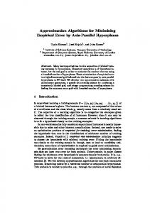
The average quality of the solutions obtained for each problem size are shown in Fig. 1. The average quality of the solutions produced by the approximation algorithm were around 50% for the small problems and increased along with the problem size. When we use LKH with the partitions derived from the approximation algorithm, the average quality decreased to around 20-40%, which is between the average quality of the solutions found by Prim and Kruskal’s algorithms. The average computation times required for each size of the problems are presented in Fig. 2, 3, and 4. The average computation times required for the approximation algorithm were less than 0.1 secs even for the relatively large problem sizes we tested; however, the LP relaxation of the multi-commodity flow model[18] needed around 100 secs for the large sized problems. The solutions found by the approximation algorithm and heuristics, and their corresponding optimal solution for an instance Ib involving three vehicles are presented in Fig.5.
Average computation time for 3 vehicles.
0.15 0.1
30
35 40 45 Total number of nodes Average computation time for 4 vehicles
50
Approx Approx+LKH Prim+LKH Kruskal+LKH
0.05 0 25
30
Fig. 4.
35 40 Total number of nodes
45
Average computation time for 4 vehicles.
50
Approximation Paths with LKH 1000
8 15
200
3
4
10 14 7
20
10 14 7
1
5
6
200
17
0
11 400
2 0
12
y
y
11 400
15
200
600 3 1
6
200
3
4 20
1000
0
1
6
5 17
2
13
500 x
Fig. 5.
10 14 7
5 17
0
12 11
400 20
2 0
15 18
16
y
y
10 14 7
400
8
800
12 4
1000
9
19
18
11
13
Optimal Paths
15
600
1
500 x
9
16
5
6
1000
8
800
20 2
Heuristic Paths by Kruskal with LKH 1000
3
4
17
depot termonal 00 1000 A F
13
500 x
19
18
16
600
12
9
19
800
18
16
600
8
9
19
800
[6] S. Rathinam, R. Sengupta, and S. Darbha, A Resource Allocation Algorithm for Multi-Vehicle Systems with Non-holonomic Constraints, IEEE Transactions on Automation Sciences and Engineering, Vol. 4, no. 1, (2007), pp. 98-104. [7] S. Rathinam, and R. Sengupta, Lower and Upper bounds for a Multiple Depot UAV Routing Problem, IEEE Control and Decision Conference (2006), San Diego, California. [8] S. Rathinam, and R. Sengupta, 3/2-approximation algorithm for two variants for a 2-Depot, Hamiltonian Path Problem, Operations Research Letters, 38(1): 63-68 (2010). [9] G. Reinelt, The Traveling Salesman-computational solutions for TSP allocations, Lecture Notes in Computer Science 840, Springer-Verlag, 1994. [10] G. Gutin, A.P. Punnen (Editors), The Travelling Salesman Problem and its variations, Kluwer Academic Publishers, 2002. [11] J. Tisdale, A. Ryan, M. Zennaro, X. Xiao, D. Caveney, S. Rathinam, J.K. Hedrick and R. Sengupta. The software architecture of the Berkeley UAV platform, IEEE Conference on Control Applications (2006), Munich, Germany. [12] V.V. Vazirani, Approximation Algorithms, Springer, 2001. [13] Graph Theory Toolbox by Sergii Iglin, 2009. [14] MatlabBGL by David Gleich, 2008. [15] J. Seik, L.Lee, and A. Lumsdaine, Boost Graph Library: The User Guide and Reference Manual. Reading, MA: Addision-Wesley Proffesional. [16] International Buisness Machines, http://www01.ibm.com/software/integration/optimization/cplex-optimizer/. [17] K. Helsgaun, LKH, July 2009, http://www.akira.ruc.dk/ keld/research/LKH/. [18] S. Yadlapalli, S. Rathinam and S. Darbha. An Approximation algorithm for a 2-Depot, Heterogeneous Vehicle Routing Problem. American Control Conference, 2009.
Heuristic Paths by Prim with LKH 1000
0
13
500 x
1000
b Solutions obtained for an instance I.
VI. C ONCLUSIONS We presented the first approximation algorithm for a variant of a Multiple Depot-Terminal Hamiltonian Path Problem when the costs are symmetric and satisfy the triangle inequality. We considered a variant of the problem where each vehicle starting from its depot should end its path at a terminal corresponding to the depot. The vehicles considered in this problem are identical dynamically. However, we consider the possibility that their capabilities or equipment available onboard could be different. Currently, the proposed algorithm for considered problem has an approximation factor of 11 3 . Future work can be include developing algorithms for more general heterogeneous vehicle routing problems with motion constraints on the vehicles, precedence and timing constraints on the targets etc. R EFERENCES [1] P. Chandler and M. Pachter. Research issues in autonomous control of tactical UAVs, Proceedings of the American Control Conference (1998), pp.394-398. [2] N. Christofides, Worst-case analysis of a new heuristic for the Traveling Salesman Problem, Technical Report 388, Graduate School of Industrial Administration, Carnegie-Mellon University, Pittsburgh, PA, 1976. [3] Hoogeveen, J. A., Analysis of christofides’ heuristic: Some paths are more difficult than cycles. Operations Research Letters, 10 (1991), pp.291-295. [4] M. Lagoudakis, V. Markakis, D. Kempe, P. Keskinocak, S. Koenig, A. Kleywegt, C. Tovey, A. Meyerson, and S. Jain, Auction-Based Multi-Robot Routing. In Proceedings of the International Conference on Robotics: Science and Systems (2005), pp.343-350. [5] W. Malik, S. Rathinam and S. Darbha, An approximation algorithm for a symmetric Generalized Multiple Depot, Multiple Travelling Salesman Problem , Operations Research Letters, Vol. 35, Issue 6, November 2007, pp.747-753.
2794