Sep 29, 2005 - bn =(â1)r 2 skck. The theory of linear recurrence equations gives the general form of the solu- tion of (17), namely aj = Aei Ïk j + Beâi Ïk j,.
Approximation of Circular Arcs by Parametric Polynomial Curves Gaˇsper Jakliˇc
Jernej Kozak ˇ Emil Zagar
Marjeta Krajnc
September 29, 2005 Abstract In this paper the approximation of circular arcs by parametric polynomial curves is studied. If the angular length of the circular arc is h, a parametric polynomial curve of arbitrary degree n ∈ N, which interpolates given arc at a particular point, can be constructed with radial distance bounded by h2 n . This is a generalisation of the result obtained by Lyche and Mørken for odd n.
1
Introduction
The approximation of circular arcs is an important task in Computer Aided Geometric Design (CAGD), Computer Aided Design (CAD) and Computer Aided Manufacturing (CAM). Though a circle arc can be exactly represented by a rational quadratic B´ezier curve (or, generally, by rational parametric curve of low degree, see [1], e.g.), some CAD/CAM systems require a polynomial representation of circular segments. Also, some important algorithms, such as lofting and blending can not be directly applied to rational curves. On the other hand, circular arcs can not be represented by polynomials exactly, thus interpolation or approximation has to be used to represent them accurately. Among others, Lyche and Mørken have studied the problem of approximation of circular segments by polynomial parametric curves (see [3]). They have found an excellent explicit approximation by odd degree parametric polynomial curves, but conjectured that the same problem with even degree could be a tough task. Their method is based on Taylor-type approximation
1
and explicitly provides parametric polynomials of odd degree n with high asymptotic approximation order, i.e., 2 n. In this paper the general case for any n ∈ N is solved. First, the approximation problem will be stated. Let � � sin ϕ f (ϕ) := , 0 ≤ ϕ ≤ α < 2 π, (1) cos ϕ be a particular parameterization of a circular arc of angular length α. It is enough to consider arcs of the unit circle only, since any other arc of the same angular length can be obtained by affine transformations. Our goal is to find a parametric polynomial curve � � xn p n := p := (2) yn of degree ≤ n with nonconstant scalar polynomials xn , yn ∈ R[t], xn (t) :=
n X
j
aj t ,
yn (t) :=
j=0
n X
bj tj ,
(3)
j=0
which provides “the best approximation” of (1). The only prescribed interpolation point is f (0) := (xn (0), yn(0))T := (0, 1)T , thus a0 := 0 and b0 := 1 in (3). In CAGD, we are interested mainly in geometric properties of objects. A particular parameterization is just a representation of an object in a desired form. Therefore the approximation error will be considered as a distance between set of points on given curves, i.e., a circular arc and a parametric polynomial in this case. It seems natural to choose a “radial distance” here (see Figure 1), i.e., o n p 2 2 d(ff , p ) := max xn (t) + yn (t) − 1 , (4) t∈I
where I is some intervalp of observation. If p is a good approximation of f on I then (4) is small and x2n (t) + yn2 (t) ≈ 1, thus p 1 |x2n (t) + yn2 (t) − 1| 2 2 p ≈ x2n (t) + yn2 (t) − 1 , = x (t) + y (t) − 1 n n 2 x2n (t) + yn2 (t) + 1
and, for computational purposes, it is enough to consider only the “error” e(t) := x2n (t) + yn2 (t) − 1 . (5) 2
1
0.5
-1
-0.5
0.5
1
-0.5
-1
Figure 1: Radial distance between circular arc (solid) and a parametric curve approximation (dashed). Ideally, e would be zero if a polynomial parameterization of circular arc would exist. But if at least one of xn or yn is of degree n, then (3) implies 6 1. x2n (t) + yn2 (t) = (a2n + b2n ) t2 n + · · · =
(6)
Now it follows from (5) that e will be small (at least for small t), if coefficients at the lower degree terms in (6) will vanish. This implies that e will be as small as possible if x2n (t) + yn2 (t) = 1 + const · t2 n .
(7)
A proper reparameterization
transforms (7) to
t → 2p n
t a2n + b2n
x2n (t) + yn2 (t) = 1 + t2 n ,
(8)
which gives 2 n nonlinear equations for 2 n unknown coefficients (aj )nj=1 and (bj )nj=1 . The paper is organised as follows. In Section 2 the system of nonlinear equations will be studied and a general closed form solution will be derived. In Section 3 the optimal asymptotic approximation order will be confirmed and in the last section some concluding remarks regarding the optimal approximation of circular arcs will be given. 3
2
Solution of the problem
Although the solutions of the system of nonlinear equations given by (8) can be obtained numerically for a particular values of n, finding a closed form solution is a much more complicated problem. In [3], authors proposed a very nice approach to solve this problem. They have used a particular rational parameterization of the unit circle to obtain the coefficients of the polynomials xn and yn . Indeed, if x0 (t) :=
2t , 1 + t2
y0 (t) :=
1 − t2 , 1 + t2
t ∈ (−∞, ∞),
(9)
is a parameterization of a unit circle, then the functions xn (t) := x0 (t) − (−1)(n−1)/2 tn y0 (t), yn (t) := y0 (t) + (−1)(n−1)/2 tn x0 (t),
are actually polynomials of degree ≤ n for which (8) holds. It is also easy to find their explicit form, but unfortunately if n is even, their coefficients are no more real numbers. However, this idea can be applied for even n too, but slightly different rational parameterization of the unit circle has to be considered. Namely, let n = 2k (2 r − 1), and let x0 , y0 be redefined as √ 2 1 − c2 t (1 − c t) , x0 (t) := 1 − 2 c t + t2
k ∈ N0 , r ∈ N,
y0 (t) :=
1 − 2 c t + (2 c2 − 1) t2 , 1 − 2 c t + t2
(10)
(11)
where c ∈ [0, 1). It is straightforward to see that x20 (t) + y02(t) = 1. Note that (9) is a particular case of (11) where c = 0. The following theorem, which has already been considered in [2] in a different context, gives one of the solutions of the nonlinear system (8) for any n in a closed form. Theorem 1 Suppose that n, k, and r satisfy (10), and let the constants ck , sk be given as ck := cos ψk and sk := sin ψk , where ψk := π/2k+1 . Further, suppose that x0 and y0 are defined by (11) with c := ck . Then the functions xn and yn , defined by �� � � � � x0 (t) xn (t) 1 (−1)r tn , (12) := (−1)r+1 tn 1 y0 (t) yn (t)
4
are polynomials of degree ≤ n that satisfy (8). Furthermore, their coefficients are given as aj =2 sk cos((j − 1) ψk ) = 2 sk Tj−1 (ck ), j = 1, 2, . . . , n − 1, an =2 sk cos((n − 1) ψk ) + (−1)r = 2 sk Tn−1 (ck ) + (−1)r ,
(13) (14)
b0 = 1, b1 = 0, bj = −2 sk sin((j − 1) ψk ) = −2 s2k Uj−2 (ck ),
(15) (16)
and
j = 2, 3, . . . , n,
where Tj and Uj are Chebyshev polynomials of the first and the second kind. Proof: The proof given here is a extended version of the proof in [2]. The equation (12) yields p 2 1 − c2k t (1 − ck t) + (−1)r tn (1 − 2 ck t + (2 c2k − 1) t2 ) xn (t) = , 1 − 2 ck t + t2 � � p (−1)r+1 tn 2 1 − c2k t (1 − ck t) + 1 − 2 ck t + (2 c2k − 1) t2 . yn (t) = 1 − 2 ck t + t2 To verify that the function xn is a polynomial of the form (3), it is enough to see that 2
(1 − 2 ck t + t ) +
n X j=3
n X j=0
aj tj = a1 t + (a2 − 2 ck a1 ) t2
(aj − 2 ck aj−1 + aj−2 ) tj + (−2 ck an + an−1 ) tn+1 + an tn+2
q = 2 1 − c2k t (1 − ck t) + (−1)r tn (1 − 2 ck t + (2 c2k − 1) t2 . A comparison of the coefficients implies the linear recurrence a1 = 2 sk , a2 = ck a1 , aj − 2 ck aj−1 + aj−2 = 0,
j = 3, 4, . . . , n − 1, (17)
with additional conditions an − 2 ck an−1 + an−2 =(−1)r , 2 ck an − an−1 =(−1)r 2 ck , an =(−1)r (2 c2k − 1). 5
(18)
Similarly, for yn it is enough to see that 2
(1 − 2 ck t + t )
n X j=0
j
bj t = b0 + (b1 − 2ck b0 ) t + n+1
n X j=2
(bj − 2 ck bj−1 + bj−2 ) tj
n+2
+ (−2 ck bn + bn−1 ) t + bn t � q � r+1 n 2 1 − c2k t (1 − ck t) + 1 − 2 ck t + (2 c2k − 1) t2 . = (−1) t Here, the conditions on bj are b1 = 0, b2 = −2 s2k , bj − 2 ck bj−1 + bj−2 = 0,
j = 3, 4, . . . , n,
(19)
and −2 ck bn + bn−1 =(−1)r+1 2 sk , bn =(−1)r 2 sk ck .
(20)
The theory of linear recurrence equations gives the general form of the solution of (17), namely aj = Aei ψk j + Be−i ψk j , where i2 := −1. From the initial conditions a1 = 2 sk = A ei ψk + B e−i ψk , a2 = 2 ck sk = A e2 i ψk + B e−2 i ψk , and the relation eiψk = ck + isk , it is easy to obtain A = sk e−i ψk and B = sk ei ψk . Therefore, aj = 2 sk cos ((j − 1) ψk ) = 2 sk Tj−1 (ck ),
j = 1, 2, . . . , n − 1.
Additional conditions (18) imply q an = 2 1 − c2k cos ((n − 1) ψk ) + (−1)r = 2 sk Tn−1 (ck ) + (−1)r . Since the general recurrence relation (19) is the same as in (17), its solution reads bj = Cei ψk j + De−i ψk j . The initial conditions b1 = 0 = C ei ψk + D e−i ψk , b2 = −2s2k = C e2 i ψk + D e−2 i ψk , 6
imply C = i sk e−iψk , D = −i sk eiψk . Hence � bj = isk eiψk (j−1) − e−iψk (j−1) = −2 sk sin ((j − 1)ψk ) = −2 s2k Uj−2 (ck ),
for j = 1, 2, . . . , n. Additional conditions (20) are satisfied and the proof is complete.
3
Approximation order
The study of the approximation order in parametric case is not a trivial task. The main problem is how the distance between parametric objects is measured. Since objects are usually considered as sets of points, the distance between sets is naturally involved. This leads to a very well known Hausdorff distance dH , which is difficult to compute in practice. As its upper bound the so called parametric distance dP has been proposed by Lyche and Mørken in [3]. Definition 1 Let f 1 and f 2 be two parametric curves defined on the intervals I1 and I2 . The parametric distance between f 1 and f 2 is defined by dP (ff 1 , f 2 ) = inf max kff 1 (φ(t)) − f 2 (t)k, φ
t∈I2
where φ : I2 → I1 is a regular reparameterization, i.e., φ′ 6= 0 on I2 . Their result will be used here to prove the following lemma. Lemma 1 Let a circular arc f be defined by (1) and its parametric approximation p by (2). Let the coefficients of xn and yn be given by (13)–(16). If p : [0, h] → R2 , where h is sufficiently small, then dH (ff , p ) ≤ dP (ff , p ) ≤ d(ff , p ) ≤ h2 n , where d is defined by (4). Proof: By [3], dP is a metric on a set of parametric curves on [0, h]. Obviously, for a particular φ, which is a regular reparameterization of f on [0, h], dP (ff , p ) ≤ max ||ff (φ(t)) − p (t)||2 . t∈[0,h]
Thus, it is enough to find a regular reparameterization φ of f for which max ||ff (φ(t)) − p (t)||2 ≤ h2 n .
t∈[0,h]
7
Let φ : [0, h] → I be defined as �
xn (t) φ(t) := arctan yn (t)
�
.
(21)
Since xn (0) = 0, yn (0) = 1 and by (13) x′n (0) = 2 sk , φ′ (0) =
x′n (0) yn (0) − xn (0) yn′ (0) = 2 sk > 0, x2n (0) + yn2 (0)
and there exists h0 > 0, such that φ is a regular reparameterization on [0, h] for 0 < h < h0 . But a point (ff ◦ φ)(t) lies on the circular arc defined by f and on the ray from the origin to p (t). This implies p ||(ff ◦ φ)(t) − p (t)||2 = | x2n (t) + yn2 (t) − 1| ≤ |x2n (t) + yn2 (t) − 1| = t2 n , where the last equality follows from (8). Finally,
max ||(ff ◦ φ)(t) − p (t)||2 ≤ h2 n
t∈[0,h]
and the proof of the lemma is complete.
An interesting question is, how large can be the angular length of the circular arc, which can be approximated by the previous method. First of all, the regularity of φ has to be assured, i.e., h has to be small enough. Then the angular length of the reparameterized circular arc f ◦ φ can be derived at least asymptotically. Lemma 2 If φ is a regular reparameterization on [0, h] defined by (21), then the length of the circular arc f ◦ φ : [0, h] → R2 is 2 sk h + O(h2 ). Proof: The proof is straightforward. The regularity of φ, (8), (13)–(16) and the fact that (1 + t2 n )−1 = 1 + O(t2 n ), simplify the arc-length to Z h Z h ′ |xn (t) yn (t) − xn (t) yn′ (t)| ′ s= k(ff ◦ φ) (t)k2 dt = dt = x2n (t) + yn2 (t) 0 0 Z h ′ xn (t) yn (t) − xn (t) yn′ (t) dt = 1 + t2 n 0 Z h (x′n (t) yn (t) − xn (t) yn′ (t))(1 + O(t2 n )) dt = 2 sk h + O(h2 ). 0
8
4
Conclusions
Since we know that the best local approximation at a particular point in the functional case is the Taylor expansion, the natural question arises how good the approximation can be, if xn and yn are taken as Taylor polynomials for sine and cosine at t = 0. The result is summarised in the following lemma. Lemma 3 Let xn and yn be the degree n Taylor polynomials of sine and cosine, respectively. Then x2n (t) + yn2 (t) = 1 + where m := and wn =
�
�
1 m t + O(tm+1 ), wn
n + 1, n is odd, n + 2, n is even,
m 2 − m2
n! if n mod 4 = 1, 2, n! otherwise.
Proof: Let Rs (t) = sin t − xn (t), Rc (t) = cos t − yn (t) be Lagrange remainders in Taylor expansions. Since x2n (t) + yn2 (t) = 1 − 2(Rs (t) sin t + Rc (t) cos t) + Rs2 (t) + Rc2 (t)
(22)
and Rs , Rc are of O(tn+1 ), it is enough to consider S(t) := −2(Rs (t) sin t + Rc (t) cos t) only. First, suppose that n is odd, i.e., n = 2 ℓ − 1. In this case the expansions of Rs and Rc are Rs (t) =
(−1)ℓ n+2 t + O(tn+4 ), (n + 2)!
therefore S(t) = −2
Rc (t) =
(−1)ℓ n+1 t + O(tn+3 ), (n + 1)!
(−1)ℓ n+1 t + O(tn+3 ). (n + 1)!
By (22), m = n + 1 and wn =
(−1)ℓ+1 (n + 1)! . 2 9
If n is even, n = 2 ℓ, (−1)ℓ n+1 Rs (t) = t + O(tn+3 ), (n + 1)! thus S(t) = −2
�
(−1)ℓ+1 n+2 Rc (t) = t + O(tn+4 ), (n + 2)!
(−1)ℓ n+2 (−1)ℓ+1 n+2 t + t (n + 1)! (n + 2)!
�
+ O(tn+4 ).
Again by (22), m = n + 2 and wn =
(−1)ℓ+1 (n + 2) n! . 2
The last lemma confirms that the Taylor polynomials are not an optimal choice if the radial distance is used as a measure of the approximation order. The construction proposed by Theorem 1 has a very small local approximation error, but only interpolates one point on a circular arc. More general results concerning the Lagrange interpolation of 2 n points on a circle-like curve by a parametric polynomial curve of degree n and the same approximation error, i.e., 2 n, are in [2].
References [1] Gerald Farin. Curves and surfaces for computer-aided geometric design. Computer Science and Scientific Computing. Academic Press Inc., San Diego, CA, fourth edition, 1997. ˇ [2] Gaˇsper Jakliˇc, Jernej Kozak, Marjeta Krajnc, and Emil Zagar. On geometric interpolation of circle-like curves. To appear. [3] T. Lyche and K. Mørken. A metric for parametric approximation. In Curves and surfaces in geometric design (Chamonix-Mont-Blanc, 1993), pages 311–318. A K Peters, Wellesley, MA, 1994.
10